RESOURCE INVESTMENT PROBLEM WITH DISCOUNTED
CASH FLOWS
A. A. Najafi
Department of Industrial Engineering, Sharif University of Technology, E-mail: [email protected]
S. T. A. Niaki
Department of Industrial Engineering, Sharif University of Technology, E-mail: [email protected]
(Received: May 18, 2004– Accepted in Revised Form: Feb. 25, 2005)
Abstract A resource investment problem is a project-scheduling problem in which the availability levels of the resources are considered as decision variables and the goal is to find a schedule, and resource requirement levels, such that some objective function optimizes. In this paper, we consider a resource investment problem in which the goal is to maximize the net present value of the project cash flows. We call this problem as Resource Investment Problem with Discounted Cash Flows (RIPDCF) and we develop a heuristic method to solve it. Results of several numerical examples show that the proposed method performs relatively well.
Key Words Project Scheduling, Resource Investment, Net Present Value, Heuristic Methods
ﻩﺪﻴﻜﭼ : ﺭﺩﺡﻮﻄﺳﻥﺁﺭﺩﻪﮐﺖﺳﺎﻫﻩﮊﻭﺮﭘﯼﺪﻨﺒﻧﺎﻣﺯﻞﺋﺎﺴﻣﺯﺍﺹﺎﺧﺖﻟﺎﺣﮏﻳﻊﺑﺎﻨﻣﺭﺩﯼﺭﺍﺬﮔﻪﻳﺎﻣﺮﺳﻪﻠﺌﺴﻣ
ﺑﺎﻨﻣ ﺱﺮﺘﺳﺩ ﻡﺎﺠﻧﺍ ﯼﺍﺮﺑ ﯼﺪﻨﺒﻧﺎﻣﺯﮏﻳ ﻦﺘﻓﺎﻳ ﻑﺪﻫ ﻭ ﺪﻧﻮﺷ ﯽﻣ ﻪﺘﻓﺮﮔ ﺮﻈﻧ ﺭﺩ ﻢﻴﻤﺼﺗ ﯼﺎﻫﺮﻴﻐﺘﻣ ﻥﺍﻮﻨﻋ ﻪﺑﻊ
ﺩﻮﺷﻪﻨﻴﻬﺑﻑﺪﻫﻊﺑﺎﺗﻪﮐﺖﺳﺍﯼﺭﻮﻃﻊﺑﺎﻨﻣﯼﺮﻴﮔﺭﺎﮐﻪﺑﺡﻮﻄﺳﻦﻴﻴﻌﺗﺭﻮﻄﻨﻴﻤﻫﻭﺎﻫﺖﻴﻟﺎﻌﻓ .
ﻪﻠﺌﺴﻣﻪﻟﺎﻘﻣﻦﻳﺍﺭﺩ
ﮊﻭﺮﭘ ﯼﺪﻘﻧﯼﺎﻫ ﻥﺎﻳﺮﺟ ﯽﻠﻌﻓ ﺺﻟﺎﺧﺵﺯﺭﺍ ﯼﺯﺎﺳ ﻪﻨﻴﺸﻴﺑ ﻑﺪﻫ ﺎﺑ ﻊﺑﺎﻨﻣ ﺭﺩ ﯼﺭﺍﺬﮔ ﻪﻳﺎﻣﺮﺳ ﯽﺳﺭﺮﺑ ﻭ ﯽﻓﺮﻌﻣﻩ
ﺪﺷﺪﻫﺍﻮﺧ ﺩﺎﻬﻨﺸﻴﭘﻥﺁ ﻞﺣﯼﺍﺮﺑ ﯼﺭﺎﮑﺘﺑﺍﺵﻭﺭﮏﻳﻭ ﺩﻮﺷﯽﻣ .
ﻪﮐ ﺪﻫﺩﯽﻣﻥﺎﺸﻧﺕﻭﺎﻔﺘﻣ ﯼﺎﻫﻥﻮﻣﺯﺁﺞﻳﺎﺘﻧ
ﺪﻨﮐﯽﻣﻞﻤﻋﺏﻮﺧﺎﺘﺒﺴﻧﯼﺩﺎﻬﻨﺸﻴﭘﺵﻭﺭ .
1. INTRODUCTION AND LITERATURE REVIEW
Project Scheduling Problem (PSP) is an investigatory area in the operations research and management science field. PSP involves finding a schedule for activities of a project subject to some side constraints such as precedent constraints, resource constraints, etc.
Many researchers have considered different variations of this problem in the past decades.
101 - Vol. 18, No. 1, February 2005 International Journal of Engineering renewable resource or non-renewable resource)
and the availability level of resources to be input parameters or decision variables. From the criteria point of view, he categorized PSPs based on the types of objective function employed. In this case, for example, minimization of the project duration, maximization of the net present value of the project cash flows, maximization of the project resource utilizations, or minimization of the project total costs introduces different PSPs. Any combination of the above viewpoints initiates different project scheduling problems. For a comprehensive survey of project scheduling problems refer to Brucker et al [2].
In this paper, we are considering a class of PSP in which the resources do exist and their availability levels are decision variables. In the literature, researchers call this problem as Resource Investment Problem (RIP). In RIP, we are concerned about completing a project which consists of a set of activities, such that a given deadline is met in time and a set of resources needed for the execution of the activities over the project is utilized. Since costs incur to provide resources, the aim is to find a schedule and resource requirement levels such that the objective function optimizes.
In the researches that undertook this problem so far, the objective function has been cost minimization. Mohring [3] introduced RIP and proved that this was NP-Hard. Also, he has proposed an exact solution method based on graph algorithms and solved some examples with 16 activities and four resources by his method. Demeulemeester [4] presented another exact algorithm for a RIP named Resource Availability Cost Problem. Akpan [5] proposed a heuristic procedure to solve RIP. Drexl and Kimms [6] presented lower and upper bounds for RIP using Lagrangian relaxation and column generation techniques. Shadrokh and Kianfar [7] developed a genetic algorithm to solve this problem and examined its performance through some test problems.
As an extension of the RIP research we encounter the RIP/max problem in the literature. In this problem the precedence constraints of RIP extends to temporal constraints where the minimum and the maximum time lags between the start of activities have to be observed in order to solve this
problem. Zimmermann and Engelhard [8] developed a time-window based branch-and-bound algorithm enumerating integral start times of activities. Nübel [9] proposed a procedure for RIP/max based on the consideration of fictitious resource capacities and the resolution of resulting resource conflicts. Nübel [10] introduced a generalization of RIP/max and developed a depth-first branch and bound procedure to solve it. Many of the recent research of project scheduling focus on maximizing the NPV of the project using the sum of positive and negative discounted cash flows throughout the life cycle of the project. It has been shown [11], for example, that a project in which progress payments are involved and which is scheduled optimally to minimize project duration may not yield the highest NPV or financial return to the firm. Russell [12] introduced the problem of the maximizing NPV in the absence of resource constraints. He proposed a successive approximation approach to solve the problem. Grin-old [13] added a project deadline to the model and formulated the problem as a linear programming problem and proposed a method to solve it. Doersch and Patterson [11] presented a zero-one integer programming model of the NPV problem. Their model included a constraint on capital expenditure of the activities in the project, while the available capital increased as progress payments were made. Bey et. Al. [14] considered the implications of a bonus/penalty structure on optimal project schedules for the NPV problem. Russell [15] considered the resource-constrained NPV maximization problem. He introduced priority rules for selecting activities for resource assignment based upon information derived from the optimal solution to the unconstrained problem. Smith-Daniels and Smith-Daniels [16] extend the Doersch and Patterson Zero-one formulation to accommodate material management costs. Icmeli
and Erengus [17] introduced a branch and bound procedure to solve
Patterson[25], Padman and Patterson[26], Padman et al[27], Ulusoy and Ozdmar[28], Padman and Smith-Daniels[29], Sepil and Ortac[30], Erengus et.al. [31], Ulusoy and Sivrikaya [32], Dayanand and Padman [33], Pinder and Marucheck [34]) To summarize, one can categorize the characteristics of the RIP model in the reviewed researches so far as:
● The objective function is cost minimization of the resource utilizations
● No payments made for the project during its life cycle
● They do not involve the concept of time-value-of-money in resource utilizations
● There is no mention on the providing and the expulsion times of the resources
Considering the fact the in real-world projects, the time-value-of-money of not only the resource utilization, but also the payments made for the project is very important for a project manager, in this research, we consider a RIP in which the goal is to maximize the Net Present Value (NPV) of the project cash flows, the cash flows being the project costs and the payments made for the project during the life cycle of the project. In this regard, we see that both the payments and the providing and expulsion times of the resources are considered. We call this problem a Resource Investment Problem with Discounted Cash Flows (RIPDCF). In section two, we define the problem precisely. Then in section three, we formulate the problem and prove it be NP-hard. In section four, we propose a heuristic solution to the problem. In order to understand the proposed solution better we provide a numerical example in section five. We measure the performance of the proposed method in section six, and finally the conclusion comes in section seven.
2. PROBLEM DEFINITION
An exact definition of the RIPDCF problem investigated in this paper is as follows: A project is given with a set of N activities indexed from 1 to N. Activities 1 and N are dummies that represent
the start and completion of the project, respectively. The activities executions need K
types of renewable resources. There are no available resources at the initial of the project, so it is necessary to provide the required levels of the resources at the activity execution time. In addition, the expulsion time of each resource type must be provided deterministically. Between the providing and the expulsion time of each resource type, availability level of the resource is equal to the provided level of the resource.
Zero-lag finish-to-start precedent constraints are imposed on the sequencing of the activities. For each activity i, the precedent activity set is denoted
as P(i). A duration Di is given where activity i is
started and it runs Di time without preemption.
Activity i uses rik units per period for resource k.
The resource usage over an activity is taken to be uniform. A cost of Ck is associated to use one unit
of resource k per period of time. In addition to
resource usage cost, each activity has some other costs such as material or overhead costs. We call these fixed costs. Fixed costs occur over activity execution and their amount at period t for activity i
is denoted by Fit. Payments are received at
payment points g∈G, where G is the set of
payment points. Payment g occurs when a set of
activities PB(g) ends, and its amount is equal to Mg. The activities are to be scheduled such that the
make span of the project does not exceed a given due date (DD). Also, α is the discount rate.
3. PROBLEM FORMULATION
To formulate the problem, let us define the decision variables as:
Si : Starting time of activity i,
i=1,2,…,N
Tg : Occurrence time for payment g,
g=1,2,…,G
Rk : Required level of resource k to be provided,
k=1,2,…,K
SRk : providing time of resource k,
k=1,2,…,K
FRk: expulsion time of resource k,
k=1,2,…,K
Xit : A binary variable where it is if activity i is
started at period t and zero otherwise, i=1,2,…,N
and t=0,1,…,DD
101 - Vol. 18, No. 1, February 2005 International Journal of Engineering
∑∑
∑∑
∑
= − − = − = − = − − = − − = K k t k FR SR t k S N i d t t it T G gge Fe e CRe
M Z Max k k i i g 1 1 1 1 0 1 )
( α α α
α (1) Or
∑
∑∑
∑
= − − − = − = + − − = − − − − = K k FR SR k k N i d t S t it T G g g e e e R C e F e M Z Max k k i i g 1 1 1 0 ) ( 1 ) 1 ( α α α α α (2) Subject to N i i P j d SSi − j ≥ j, ∀ ∈ (), =1,2,..., (3)
DD
SN ≤ (4)
G g g PB i d S
Tg ≥ i+ i, ∀ ∈ ( ), =1,2,..., (5)
K k k PR i S
SRk≤ i, ∀ ∈ ( ), =1,2,..., (6)
K k k UR i d S
FRk≥ i+ i, ∀ ∈ ( ), =1,2,..., (7)
K k DD t R x r k N i t d t l il ik i ,..., 2 , 1 , ,..., 2 , 1 , 0 , 1 1 = = ≤
∑ ∑
= =− + (8) N i xit LS ES t i i ,..., 2 , 1 , 1 = =∑
= (9) N i tx S i i LS ES t iti=
∑
, =1,2,...,=
(10)
i
it i N LS
X ={0,1}, =1,2,..., , t=ESi,..., (11) N
i
Si ≥0, =1,2,..., (12)
K k
Rk ≥0, =1,2,..., (13)
K k
FR
SRk, k ≥0, =1,2,..., (14)
G g
Tg ≥0, =1,2,..., (15)
Where, ESi is the earliest start of activity I, LSi is
the latest start of activity i, PR(k) is an activity set
that uses resource k and has no precedence, and UR(k) is an activity set that use resource k and has
no successor.
The objective function (1) maximizes the net present value of the project. It includes positive effects of the present values of the payments, negative effects of the present values of the fixed costs and negative effects of the present values of the costs for providing the resources. Equation (3) enforces the precedent relations between activities. Constraint (4) ensures that the project ends by the latest allowable completion time. Equation (5) guarantees that payments occur when required activities have been finished. Constraints (6) and (7) correspond to the providing and the expulsion times of the resources. Equation (8) ensures that
the provided resource units are sufficient to implement the schedule. Equation (9) states that every activity must be started only once. Equation (10) states the relationship between variables Sj
and variables Xit. Sets of constraints (11), (12),
(13), (14) and (15) denote the domain of the variables.
One can convert the RIPDCF to RIP with some simplifications. For example, if we eliminate the constraints (5), (6), (7), and (14) and reduce the non-linear objective function to a linear one, where the aim is to minimize the make-span of the project, then a RIP could be reached. Mohring proved that RIP is NP-hard [3]. Since the RIPDCF is convertible to RIP with some simplification, then RIPDCF in also NP-hard.
4. A SOLUTION PROCEDURE
In this section, based on the priority rules of the RIPDCF we propose a heuristic method to solve the problem. To do this, first we state some definitions that are required in the procedure.
Definition 1:
Negative cash flow of an activity: Includes discounted cash flow of the resource usage cost and fixed cost at the activity starting time. It can be stated as:
∑
∑
∑
∑
∑
= = − − − = − − = − − = − − − − − − = − − = K k K k d k ik d t t it d t t k ik d t t it i e e C r e F e C r e F CF i i i i 1 1 1 0 1 0 1 0 ) 1 1 ( α α α α α (16) Definition 2:Positive cash flow of an activity: If the precedent activity set of payment occurrence contains only one activity, then we set a positive cash flow of the activity to be equal to the discounted cash flow of that payment at the activity starting time. In this case, we define the positive cash flow of the activity as:
i
d g
i M e
increase to M. In the following sections we denote
the number of activities by M.
Definition 3:
Cash flow of an activity: Cash flow of an activity equals to the sum of the negative and the positive cash flows of an activity. In other words, we have:
+ −+
= i i
i CF CF
CF (18)
Definition 4:
The amount of non-usage resource at a period: With equation (8) modified, the amount of non-usage resource k at a period t, Wkt , can be obtained
by: k kt M i t d t l il
ikx W R
r
i
= +
∑ ∑
=1 =− +1(19) Where,
0
1 2
0 1 2
kt
W
≥
,
k
=
, ,..., K ,
t
=
, , ,..., DD
(20) Now, we simplify the problem formulation in the following form:∑∑
∑
= − − = − = − = K k t kt FR SR t k S M iie CWe
CF Z Max k k i 1 1 1 α
α (21)
Subject to Equations (3), (4), (6), (7), (19), (9), (10), (11), (12), (13), (14) and (20).
In order to develop the solution procedure, we use the double structure of the objective function given in (21). The double structure includes positive roles of the activities cash flow, ( Si
M
i i
e
CF
−α =∑
1
), and the negative roles of the non-usage resource costs, (
∑ ∑
= − − = K k t kt FR SR tkW e C k k 1 1 α ).
Now we are ready to describe the executive steps of the proposed algorithm as follows:
Step1: Let problem P be the RIPDCF that we are interested to solve and Psub be a problem obtained by removing resources of the P problem. Therefore, the Psub problem can be reached from the P problem by removing resource constraints and negative roles of non-usage resource costs in objective function. The Psub problem can be described as follows:
i
S M
i i
sub CFe
Z
Max −α
=
∑
=1
(22) Subject to Equations (3), (4), and (11).
The Psub problem is a project scheduling problem with discounted cash flows and can be solved exactly [12]. Call the acquired problem as Active Problem, solve it by related methods, and obtain the optimum value of its objective function. Call the optimum solution as active scheduling. Now, enter the resource at active scheduling and determine the maximum of usage level for each type of resources. If we set the required level of each provided resource equal to the maximum of usage level of the resources, then the active scheduling is a feasible solution for the P problem and you can obtain the providing and expulsion time of each resource and obtain the discounted non-usage cost of each resource from the following equation: t kt FR SR t k
k C W e
U k k α − − =
∑
= 1 (23) Determine the objective function value of the master problem at this solution by the following expression and call it the active objective function value.∑
= − = K k k Sub U Z Z 1 (24)Step 2: Add all resources in a set, named resource
candidate list.
Step 3: From the list of resource candidates, select
the resource with the highest discounted cost of non-usage (Uk).
101 - Vol. 18, No. 1, February 2005 International Journal of Engineering bound of the resource using the following
expression:
⎪ ⎪ ⎭ ⎪⎪ ⎬ ⎫
⎪ ⎪ ⎩ ⎪⎪ ⎨ ⎧
× =
= =
∑
} r { Max , DD
) d r (
Max
R ik
M , ... , i M
i
i ik
k 1
1 (25)
Step 4: If the temporary objective function value is
more than the active objective function value and the project is finished before its deadline, add the selected constraint to the active problem. Then, consider the acquired problem, related scheduling, and the temporary objective function value as an active problem and go to step three. Otherwise, do not add the selected resource constraint to the active problem.
Step 5: Eliminate the selected resource from the
resource candidate list and go to step six.
Step 6: If the resource candidate list is empty,
stop. The active schedule is the solution of the proposed algorithm. Otherwise, go to step three.
5. A NUMERICAL EXAMPLE
In order to illustrate the proposed method, consider a project network with eight activities and three
resources. Figure 1 shows the activity-on-node representation of the network with the node numbers denoting the activity numbers. We define activity 1 and 8 to be dummies. Table 1 presents the durations, the resource requirements, and the fixed costs of the activities. The providing costs of the resources per period of time are 3, 2, and 4 respectively. The deadline is 8 and the discount rate is taken to be 0.01 per period. There are three payments as follows: 40 after the end of activity 2, 20 when activity 4 finishes, and 90 after the end of activity 7.
Figure 1: The Project Network of the Example Problem
In order to solve this problem, first we calculate the cash flows of the activities by equations (16), (17) and (18), as shown in Table 2.
1
2 3
4 5
6
7 8
Table 1: Activity Data of the Example Problem
Fixed costs Resource requirements
Fi2
Fi1
ri3
ri2
ri1
Duration (di) Activity
(i)
- -
0 0
0 0
1
5 5
1 0
2 2
2
1 3
0 2
1 2
3
- 5
1 1
0 1
4
9 13
1 2
1 2
5
1 1
2 0
1 2
6
- 6
1 1
0 1
7
- -
0 0
0 0
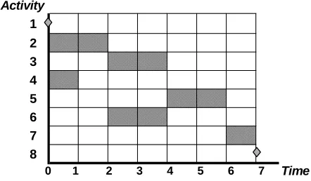
Figure2: The Active Schedule (Stage 1)
ow, we follow the steps in the proposed procedure. According to step 1, we solve the problem without considering the resources. We call the corresponding problem an active problem and
define its solution as an active schedule. Figure 2 shows the active schedule of the problem.
For this schedule the value of the objective function, Zsub, is 37.7. Then, we obtain the
requirement level, the providing and expulsion time of each resource. In addition, we calculate the discounted costs of the non-usages by equation (23). Table 3 shows the results.
From equation (24), we obtain the objective function value of the master problem at this solution (active objective function value (Z)) as -19.4. Now, according to step 2 of the procedure, the list of the resource candidates contains all three resources. In step 3, since the discounted cost of non-usage of resource 3 is the highest, we select resource 3. Furthermore, since the providing level of resource 3 has not reached its lower bound, we decrease its requirement level to 2. Then, we solve the active problem with the resource 3 added as a constraint. Figure 3 shows the solution.
Table 2: Activity Cash Flows of the Example Problem
Cash flow
(CFi)
Positive cash flow
(CF+ i)
Negative cash flow
(CF -i)
Activity (i)
0
0
0
1
20
40
-20
2
-20
0
-20
3
10
20
-10
4
-40
0
-40
5
-10
0
-10
6
80
90
-10
7
0
0
0
8
Activity
1 2 3 4 5 6 7 8
Time
101 - Vol. 18, No. 1, February 2005 International Journal of Engineering For this solution, Zsub is 37.4. Then, we obtain the
resource plan again according to the schedule. Table 4 shows the results.
In this solution, we obtain the objective function value of the master problem as 19.9. Since the objective function value of this solution is more than the active objective function value and the project finishes before its deadline, according to step four of the algorithm we add the mentioned constraint to the active problem. Furthermore, the active schedule is now changed and is shown in Figure 3.
Now from the candidate list we select resource 3 in step three because of its highest non-usage cost (7.8). However, its lower bound is equal to its requirement level (2) and we cannot decrease it. Therefore, we eliminate this resource from the candidate list, select resource 1, and decrease its level to two. Then, we solve the active problem by adding resource 1 as a constraint. Figure 4 shows the schedule.
For this solution, Zsub is 37.4. Then, we obtain the
resource plan again according to the schedule. Table 4 shows the results.
In this solution, we obtain the objective function value of the master problem as 19.9. Since the objective function value of this solution is more than the active objective function value and the project finishes before its deadline, according to step four of the algorithm we add the mentioned
constraint to the active problem. Furthermore, the active schedule is now changed and is shown in Figure 3. Now from the candidate list we select resource 3 in step three because of its highest non-usage cost (7.8). However, its lower bound is equal to its requirement level (2) and we cannot decrease it. Therefore, we eliminate this resource from the candidate list, select resource 1, and decrease its level to two. Then, we solve the active problem by adding resource 1 as a constraint. Figure 4 shows the schedule.
We obtain the objective function value of the master problem as 12.4 for this schedule. Since it is less than the active objective function value, according to step four, we go
Figure 3: The Project Schedule (Stage 2) Table 3: The Resource Plan of the Active Schedule (Stage 1)
Resource No. (k) Requirement Level
(Rk)
Providing Time (SRk)
Expulsion Time (FRk)
Discounted Cost of Non-Usage (Uk)
1 3 0 5 14.6
2 4 2 6 11.6
3 3 0 6 30.9
Activity
1
2 3 4 5 6 7
8
Time
0 1 2 3 4 5 6
Table 4: The Resource Plan of the Schedule (Stage 2)
Resource No. (k) Requirement Level ( Rk)
Providing Time (SRk)
Expulsion Time (FRk)
Discounted Cost of Non-Usage (Uk)
Figure 4: The Project Schedule (Stage 3)
to step five and we ignore the constraint of resource 1 and eliminate this resource from the candidates list. Since the candidate list is not empty we go to step three. The candidates list now contains resource 2 only. However, its lower bound is equal to 2 and cannot be decreased. Hence, we eliminate this resource from the candidate list according to step five. Now, the candidate list becomes empty and the procedure terminates in step six. The current active schedule shown in Figure 3 is the solution of the proposed algorithm for the given RIPDCF problem
6. THE PERFORMANCE OF THE PROPOSED PROCEDURE
In this section, we present the performance of the proposed procedure introduced in the previous sections. To do this, first, we generate some test problems and then we present the computational results of the proposed method applied to the test problems.
6.1. The Test Problems
Since the RIPDCF is a newly defined problem, we cannot find any standard test problems to examine the performance of the proposed procedure introduced in this paper. Therefore, we generate a set of 220 test problems containing different instances using ProGen software package [35]. ProGen is an instance generator for a broad class of resource-constrained project scheduling problem by varying three factors: network complexity, resource factor, and resource strength. The network complexity reflects the average number of immediate successors of an activity. The resource factor is a measure of the average number of resources requested per activity. The resource strength describes the scarceness of the resource capacities. These factors are known to have a big impact on the hardness of a project instance [35]. Although the Progen software is not capable of creating some instances of the RIPDCF problem, we develop our own instance generator program in the following manner:
1. We consider the project deadline (DD) being a
random variable uniformly distributed between 1.2*ETP and 1.6*ETP, where ETP is the earliest
finish time of the project, and we generate its sample values accordingly.
2. The providing costs of resources (Ck’s) are set
equal to the resource availability levels generated by ProGen.
3. The fixed cost of activity i in period t, (Fit), is
calculated by the ratio of the resource costs of the activity and is generated from uniform distribution on [0, 0.3*RCAi], where RCAi is obtained from the
following equation:
∑
∑
∑
= = −
− −
=
−
− − =
=
K
k
K
k
d k
ik d
t
t k ik i
e e C r e
C r RCA
i i
1 1
1
0
) 1 1
( αα
α (25)
Table 5: Resource Plan for Schedule (Stage3)
Resource No. (k) Requirement Level ( Rk)
Providing Time (SRk)
Expulsion Time (FRk)
Discounted Cost of Non-Usage (Uk)
1 2 1 6 5.7
2 2 0 7 3.8
3 2 0 7 15.4
Activity
1 2 3 4 5 6 7 8
Time
101 - Vol. 18, No. 1, February 2005 International Journal of Engineering 4. In order to generate the payment values, first, we
deterministically select the terminal activity and randomly select the other activities based on a uniform distribution on the interval (0.2, 0.5). Then we randomly distribute a multiple (uniformly distributed in the interval (1.5, 2.5)) of the total activity costs to the selected activities.
We implement the proposed method to different scenarios generated based on the above instance generator. In these scenarios, we consider the number of activities in the network to be less than 10, 10, 15, 20, 30, and 60, the number of resources to be 3, 4, or 5, the network complexity to be 1.5, and the resource factor and the resource strength to be 1 and 0.2, respectively. Activity durations and resource requirements are integer values out of [1, 10] uniformly distributed. We set the discount rate to be equal to 0.01, 0.015, and 0.02. We apply the method to 220 instances by the instance generator described above.
6.2. The Computational Results
In this section, we report the results obtained by examining the proposed procedure to the generated test problems. To do this, first, we coded a Matlab computer program of the procedure, and then we employed the program on the test problems. To evaluate the performance of the procedure we needed some good solutions. Since there was no other existing procedure to solve the RIPDCF problem, we solved the mathematical modeling of the test problems with solver software (LINGO). However due to the nature of the problem, LINGO [36] was unable to obtain a global optimal solution for all the test problems. In these cases, we assumed that the solution obtained by LINGO was a good one to compare with. We performed the experiments on a PC with a Pentium 1800 processor and 64 MB RAM, limiting the solution
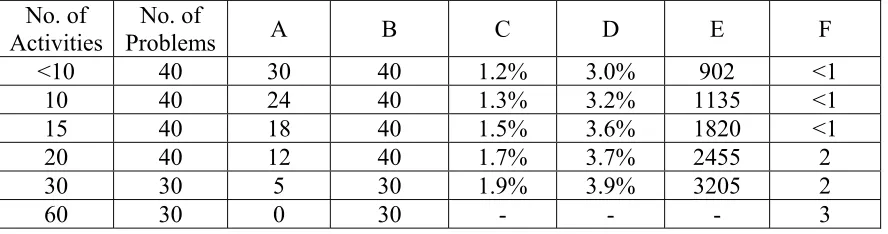
time less than or equal to 3600 CPU seconds. Table 6 contains a summary of the computational results.
We define the columns of table 6 as follows:
A: Number of problems in which LINGO was able
to find a solution
B: Number of problems in which the proposed
procedure found a solution
C: Average of the relative deviation percentages
for instances solved by LINGO, where a relative deviation percentage is obtained by equation (26).
Objective Function Value in LINGO – Objective Function Value in the Proposed Procedure _______________________________________
Objective Function Value in LINGO
D: Maximum of the relative deviation percentages
for instances solved by LINGO, where a relative deviation percentage is obtained by equation (26).
E: Average CPU time (in seconds) required to
obtain the solutions by LINGO
F: Average CPU time (in seconds) required to
obtain the solutions by the proposed method. The results of Table (6) show that
a. There are many instances that the solver software is unable to solve, but there is a solution by the proposed method.
b. The relative deviation percentages for the instances solved by LINGO are not high. It means that there is no significant difference between the solutions obtained by LINGO and the ones obtained by the proposed method.
c. While actually there is no difference between the solutions obtained by LINGO and the proposed method, the amount of CPU time for the proposed method is much less than that of those obtained by LINGO.
Table 6: Computational Results
No. of
Activities
No. of
Problems
A B C D E F
<10 40 30 40 1.2%
3.0%
902 <1
10 40 24 40
1.3%
3.2%
1135
<1
15 40 18 40
1.5%
3.6%
1820
<1
20 40 12 40
1.7%
3.7%
2455 2
30 30 5 30
1.9%
3.9%
3205 2
7. CONCLUSIONS AND
RECOMMENDATIONS FOR FUTURE RESEARCH
In this paper, we introduced a new resource investment problem in which the goal was to maximize the discounted cash flows of the project payments. We mathematically formulated the problem and showed that it is a Np-hard problem. In order to solve the problem we came up with a heuristic approach and through some generated test problems, we showed that it works relatively well. Some extensions of this research might be of interest. While in this paper we only considered the "payments at pre-specified event nodes", some other payment models such as progress payments and payments at pre-specified time points may be considered in the project. The other extension of this research would be to investigate a RIP/max problem in which the goal is to maximize the NPV of the project. One of the other potential interests would be to develop some meta-heuristics methods, such as genetic algorithm, simulated annealing, neural networks, ant ant-colony algorithm, etc., to solve the RIPDCF problem.
8. REFERENCES
1. Tavares, L.V. ,”A Review of the Contribution of Operation Research to Project Management”, European Journal of the Operational Research, 136(2002), 1-18.
2. Brucker, P., Drexl, A., Mohring, R., Neumann, K. and E. Pesch, “Resource-Constrained Project Scheduling: Notation, Classification, Models and Methods”, European Journal of Operational Research, 112(1999), 3-41.
3. Mohring, R.H. ,”Minimizing Costs of Resource Requirements in Project Networks Subject to A Fix Completion Time”, Operational Research, 32(1984),89-120.
4. Demeulemeester, E. L. , “Minimizing Resource Availability Costs in Time Limited Project Networks”. Management Science, 41(1995), 1590-1598.
5. Akpan, E.O.P. , “Optimal Resource Determination for Project Scheduling” ,Production Planning and Control, 8(1997), 462-468.
6. Drexl, A. and A. Kimms , “Optimization Guided Lower & Upper Bounds for the Resource Investment Problem”, Journal of the Operational Research Society, 52(2001), 340-351.
7. Shadrokh, S. and F. Kianfar , “A Genetic Algorithm for Resource Investment Problem, Enhanced by Revised Akpan Method”, Working Paper, Industrial Engineering Department, Sharif University of Technology, Iran, 2002.
8. Zimmermann, J. and H. Engelhardt, “Lower Bounds and Exact Algorithms for Resource Leveling Problems”, Technical Report 517, University of Karlsruhe, Germany, 1998.
9. Nübel, H., “A Branch and Bound Procedure for the Resource Investment Problem subject to Temporal Constraints”, Technical Report 574, University of Karlsruhe, Germany, 1999.
10. Nübel, H., “The Resource Renting Problem Subject to Temporal Constraints”, O. R Spektrum, 23(2001), 574-586.
11. Doersch, R. H., J. H. Patterson, “Scheduling a Project to Maximize its Present Value: Zero- One Programming Approach”, Management Science, 23(1977), 882- 889.
12. Russell,A.H., “Cash Flows in Networks”, Management Science, 16(1970),357-373.
13. Grinold,R.C. , “The Payment Scheduling Problem”, Naval Research Logistics Quarterly, 19(1972), 123-136.
14. Bey, R.B., R.H. Doersch and J.H. Patterson, "The Net Present Value Criterion: Its Impact on Project Scheduling", Project Management Quarterly, 12(1981), 223-233.
15. Russell, R.A.,”A Comparison of Heuristics for Scheduling Projects with Cash Flows and Resource Restrictions”, Management Science, 32(1986), 291-300.
16. Smith-Daniels, D.E. and V.L. Smith-Daniels ,” Maximizing the Net Present Value of a Project Subject to Materials and Capital Constraints”, Journal of Operations Management, 7(1987),33-45.
17. Icmeli, O. and S.S. Erenguc,”A Branch and Bound Procedure the Resource-Constrained Project scheduling Problem with Discounted Cash Flows”, Management Science, 42(1996), 1395-1408.
101 - Vol. 18, No. 1, February 2005 International Journal of Engineering Present Value of Projects” , European Journal of
Operational Research,49(1990),35-49.
19. Demeuemeester,E. , W. Herroelen & P. Van Dommelen, “ An Optimal Recursive Search Procedure for the Deterministic Unconstraind Max-npv Project Scheduling Problem”, Research Report 9603,Department of Applied Economics, K.U. Leuven, 1996.
20. Sepil, C. B.Kazaz, “Project Scheduling with Discounted Cash Flows and Progress Payments”, Working Paper, Middloe East Technical University,1995.
21. Smith-Daniels, D.E. “Summary Measures for Predicting the Net Present Value of a Project”, Working Paper, College of St. Thomas, St. Pual, Minnesota,1986.
22. Baroum, S.M., “An Exact Solution Procedure for Maximizing The Net Present Value of Resource-Constrained Projects”, Unpublished Ph.D. dissertation, Indiana University, 1992.
23. Yang, K.K. , F.B. Talbot and J.H. Patterson, “Scheduling a Project to Maximize Its Net Present Value: An Integer Programming Approach” , European Journal of Operational Research, 64(1992),188-198.
24. Smith-Daniels, D.E. and N.J. Aquilano, “Using a Late Start Resource Constrained Project Schedule to Improve Net Present Value”, Decision Sciences, 18(1987), 617-630.
25. Baroum, S.M. and J.H. Patterson, “The Development of Cash Flow Weight Procedures for Maximizing The Net Present Value of a Project”, Journal of Operation Management, 14(1996), 209-227.
26. Padman, R. and J.H. Patterson, “ A Comparative Evaluation of Cash Flow Weight Heuristics for Maximizing the Net Present Value of a Project”, Working Paper, King Abdul Aziz University, 1993.
27. Padman, R. D.E. Smith-Daniels and V.L. Smith-Daniels ,” Heuristic Scheduling of
Resource-Constrained Project scheduling Problem with Discounted Cash Flows: An Optimization-Guided Approach”, Working Paper 90-6,arnegie-ellon University, January 1990.
28. Ulusoy, G., L. Ozdamar ,“A Heuristic Scheduling Algorithm for Improving The Duration and Net Present Value of a Project”, International Journal of Operations & Production Management, 15(1995), 89- 98.
29. Padman,R. and D.E. Smith-Daniels,” Maximizing the Net Present Value of Capital Constrained Projects: An Optimization Guided Approach”, Working Paper 93-56,Carnegie Mellon University,September 1993.
30. Sepil, C. and N. Ortac, "Performance of the Heuristic Procedures for Constrained Projects with Progress Payments", Journal of the Operational Research Society, 48(1997), 1123-1130.
31. Erenguc,S.S. , S. Tufekei and C.J. Zappe,” The Solution of the Time/Cost Trade-Off Problem with Discounted Cash Flows Using Generalized Benders Decomposition”, Research Report, University of Florida,1991.
32. Ulusoy, G. and F.Sivrikaya,” Four Payment Models for the Multi-mode Resource Constrained Project Scheduling Problem with Discounted Cash Flows”, Accepted for publication in Annals of OR, March 2001.
33. Dayanand, N., R. Padman, "On Modelling Payments in Projects", Journal of the Operational Research Society, 48(1997), 906- 918.
34. Pinder, J.P. and A.S. Marucheck, “Using Discounted Cash Flow Heuristics to Improve Project Net Present Value”, Journal of Operation Management, 14(1996), 229-240.
35. Kolish, R., Sprecher, A. and A. Drexl, “Characterization and Generation of a General Class of Resource-Constrained Project Scheduling Problems", Management Science, 41(1995), 1693-1703.