TECHNICAL NOTE
INTEGRATED APPROACH FOR CELLULAR
MANUFACTURING – A CASE STUDY
B. S. Nagendra Parashar and Ramprasad Kamath
Mechanical Engineering Group, Birla Institute of Technology and Science Pilani, Dubai Campus, Dubai, UAE, [email protected]
H.V. Somasundar
Sri Krishna Institute of Technology Bangalore, India, [email protected]
(Received: August 12, 2002 – Accepted in Revised Form: December 8, 2003)
Abstract To cope with fast changing customer requirements, industrial demands and to meet stringent specifications of customers Cellular Manufacturing Systems has become an effective tool in hands of manufacturers. Most of the published literature on cell formation earlier considers only the data available in the route sheets and ignored subproblems associated with cell formation. There is a need to develop an integrated approach for Cellular Manufacturing, which considers all the aspects. Present paper focuses on developing an integrated approach for Cellular Manufacturing. Proposed method considers workload, volume of production and processing times for machine cell and part family formation, which was ignored by past researchers. Proposed method has been tested on one of the largest public sectors in Asia and the benefits that can be obtained by implementation are reported.
Key Words Cellular Manufacturing, Machine Cells, Part Family, Exceptional Component, Workload Index, Cellular Layout
ﻩﺪﻴـﻜﭼ
ﻩﺪﻴـﻜﭼ
ﻩﺪﻴـﻜﭼ
ﻩﺪﻴـﻜﭼ
ﻥﺩﺭﻭﺁﺮﺑﻱﺍﺮﺑﻭﺖﻌﻨﺻﺖﺳﺍﻮﺧﺭﺩﻭﻱﺮﺘﺸﻣﻱﺎﺿﺎﻘﺗﺭﺩﻊﻳﺮﺳﺕﺍﺮﻴﻴﻐﺗﻪـﺑﻲﻳﻮﮕﺨـﺳﺎﭘﺭﻮﻈﻨـﻣﻪـﺑ
ﻲﻣﻱﺮﺛﻮﻣﺭﺍﺰﺑﺍﺭﺍﻭﻩﺮﺠﺣﺪﻴﻟﻮﺗﻱﺎﻬﻤﺘﺴﻴﺳﻪﻛﺪﻧﺍﻪﺘﻓﺎﻳﺭﺩﻥﺎﮔﺪﻨﻨﻛﺪﻴﻟﻮﺗ،ﺯﺎﻴﻧﺩﺭﻮﻣﻖﻴﻗﺩﺕﺎﺼﺨﺸﻣ
ﺪﺷﺎﺑ . ﺮﺘﺸﻴﺑ
ﺑﺭﺩﺩﻮﺟﻮﻣﻱﺎﻫﻩﺩﺍﺩﻪﺑﺎﻬﻨﺗﺎﻫﻩﺮﺠﺣﻞﻴﻜﺸﺗﻩﺭﺎﺑﺭﺩﻩﺪﺷﭖﺎـﭼﺕﻻﺎـﻘﻣ
ﻲﻣﺭﺎﻛﺮﻴﺴﻣﻱﺎﻬﮔﺮ
ﻞﺋﺎﺴﻣﻭﺪﻧﺯﺍﺩﺮﭘ
ﺪﻧﺭﺍﺪﻧﺮﺑﺭﺩﺍﺭﺎﻫﻩﺮﺠﺣﻞﻴﻜﺸﺗﻲﮕﻧﻮﮕﭼﺰﻳﺭ
.
ﻪﻛﺭﺍﻭﻩﺮﺠﺣﺪﻴﻟﻮﺗﻱﺍﺮﺑﻊﻣﺎﺟﻭﻪﭼﺭﺎﭙﻜﻳﻩﺎﮔﺪﻳﺩﻚﻳﻭﺭﻦﻳﺍﺯﺍ
ﺩﻮﺑﺪﻫﺍﻮﺧﻩﺪﻧﺯﺎﺳ،ﺪﺷﺎﺑﺐـﻧﺍﻮﺟﻪـﻤﻫﻩﺪﻧﺮﻴـﮔﺮـﺑﺭﺩ
.
ﻲﻣﺎﺘﺳﺍﺭﻦﻳﺍﺭﺩﻲﺷﻼﺗﻪﻟﺎﻘﻣﻦﻳﺍ
ﺪﺷﺎﺑ . ،ﻱﺭﺎﻛﺭﺎﺑﻲﻨﻌﻳ
ﺵﺭﻭﺍﺮﻓﻥﺎﻣﺯ،ﺪﻴﻟﻮﺗﻢﺠﺣ
ﻲﻣﺭﻮﻈﻨﻣﺍﺭﺕﺎﻌﻄﻗﻩﺩﺍﻮﻧﺎﺧﻞﻴﻜﺸﺗﻭﻩﺮﺠﺣﺮﻫﺭﺩﻦﻴﺷﺎﻣ
ﺩﺭﺍﺩ .
ﻱﺩﺎﻬﻨﺸﻴﭘﺵﻭﺭﻦﻳﺍ
ﺪﻳﺪﺟﺵﻭﺭﻦﻳﺍﺩﺮﺑﺭﺎﻛﺯﺍﻩﺪﻣﺁﺖﺳﺪﺑﺞﻳﺎﺘﻧﻭﻩﺪﺷﻩﺩﻮـﻣﺯﺁﺎﻴـﺳﺁﻲـﻣﻮﻤﻋﻱﺎﻬـﺸﺨﺑﻦـﻳﺮﺘﮔﺭﺰﺑﺯﺍﻲـﻜﻳﻱﻭﺭ
ﺖﺳﺍﻩﺪﺷﺵﺭﺍﺰﮔ
.
1. INTRODUCTION
Cellular Manufacturing has been gaining importance for both practitioners and researchers in the area of manufacturing during the last decade. It is one of the strategies the organization should adopt before implementing new technologies like Computer Integrated Manufacturing, Flexible Manufacturing
aggressively at global level by improving manufacturing flexibility, quality and at the same time reducing lead-time and manufacturing costs simultaneously.
The basic idea in Cellular Manufacturing is to group parts that have similar processing needs into part families, and machines that meet these needs into machine cells. Each machine cell is dedicated to the manufacture of a part family. The advantages of Cellular Manufacturing over traditional manufacturing are many folds. To mention a few of them reduced setup time, work-in-process inventory, lead-time, simplified flow of materials, improved human relations etc. Cellular Manufacturing combines the efficiency of a flow shop layout with the flexibility of a job shop layout.
The first problem that must be addressed when considering a Cellular Manufacturing is that of cell formation. The cell formation method is of paramount importance when implementing a Cellular Manufacturing because the success of Cellular Manufacturing depends greatly on the initial grouping of machines and parts. Ever since the concept of Cellular Manufacturing is introduced attempts were made by different researchers and practitioners to develop algorithms for the efficient cell formation. Few of them include the application of classification and coding systems, flow analysis, similarity coefficient methods, mathematical models, graph theory models, genetic algorithms, neural networks, fuzzy sets theory etc. All the cell formation techniques mentioned above have their own limitations. Mathematical models Srinivasan [1], Crama and Ostan [2], Jayakrishanan [3] et al. are all characterized by week continuous relaxations, and hence, are not well suited for the solution to optimality of large-scale problems. For large-large-scale problems their usefulness is purely illustrative. Similarity coefficient method is among the most frequently cited approach to cell formation problems. Several measures of similarity among machines and parts have been proposed in the last three decades. Applications of similarity coefficient to cell formation include the contributions of McAuley [4], Waghodekar and Sahu [5], Nagendra Parashar and Somasundar [6] etc. Similarity coefficient methods are more flexible in incorporating manufacturing data into the machine cell formation.
The similarity coefficient method lends itself more easily to computer applications.
There is a need to develop a cell formation technique, which can handle multiple objectives pertinent to Cellular Manufacturing such as minimization of work-in-process inventory, material handling, setup time, maximization of machine utilization etc. Most of the published literature addresses the problem of cell formation alone and ignores processing of exceptional components (components required to be processed in more than one cell), arranging cells and machines within the cells, production control activities etc.
The paper presented here is an integrated approach for Cellular Manufacturing. Present paper deals with new heuristics along with similarity coefficient for machine cell and part family formation. Processing of exceptional components and Cellular layout are also dealt with. Proposed method is tested on 20-machine 144-component problem in one of the largest public sectors in India.
2. PROBLEM STATEMENT
The problem under consideration is taken from one of the largest public sectors in India, which is regarded as one of Asia’s leading corporate giants. The company faced the problems of having increased material handling, larger setup times (as high as 15-20 times processing time), higher work-in-process inventory, longer lead-time, queue time, difficulty in meeting delivery schedules etc. To overcome these problems company resorted to apply Cellular Manufacturing.
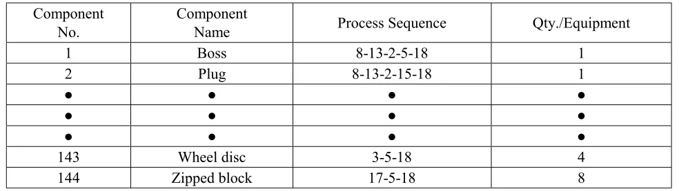
type having close dimensional tolerances and good surface finish. The number of manufacturing operations carried out varied from 1 to 8. Process sequence for the components is shown in Table 1.
3. METHODOLOGY
The problem under consideration is having large number of components for processing on different machine tools (refer to Table 1). For the reasons mentioned earlier straightforward application of any of the cell formation methods discussed earlier might have not resulted in efficient machine cell. In this paper we have combined similarity coefficient with simple heuristics to obtain an optimal solution. Proposed method is an integrated approach for cell formation, processing exceptional components and arrangement for Cellular layout. Present work is an extension of work done by Nagendra Parashar and Somasundar [6]. Proposed method considers workload of machines, utilization and cost parameters, which was ignored by past researchers. Proposed method is explained below.
Step 1
Represent the data in the form of machine-component incidence matrix:Represent the data given in Table 1 in the form of machine-component incidence matrix with machines in row and components in column position (not shown). Enter ‘1’ if the machine ‘0’
processes a particular component otherwise go to Step 2.
Step 2
Compute similarity coefficient between all machines using the formula [6]:1
SC
ij=
if
i
=
j
(
)
( )
∑
∑
= =
×
=
nj1 p
ip nj
1 p
jp ip
ij
a
a
a
SC
if
i
≠
j
(1)aip = 1 if component is processed by the machine, ‘0’ otherwise.
nm
,...,
2
,
1
i
nj
,...,
2
,
1
j
=
=
where nj = number of jobs and nm = number of machines.
The similarity coefficient varies from 0 and 1. ‘0’ similarity coefficient implies machines within the cell are purely dissimilar and they do not have a single common machining operation. Similarity coefficient ‘1’ implies machines have complete common operations.
Step 3
Categorize machines into ideal, critical and non-critical machines.TABLE 1. Components and its Process Sequence for WA-200 Project.
Component No.
Component
Name Process Sequence Qty./Equipment
1 Boss 8-13-2-5-18 1
2 Plug 8-13-2-15-18 1
● ● ● ●
● ● ● ●
● ● ● ●
143 Wheel disc 3-5-18 4
Identify number of components associated with different machines and number of machines available. This is shown in Table 2.
Now, categorize machines as critical, non-critical and ideal machines as per the following guidelines from the data available in Table 2.
Critical Machines
Only a few machines of this type are available and are associated with processing of large number of components viz. radial drillingmachine, vertical milling machine etc.
Ideal Machine
Machines are less in number, and they process a few components viz. H-22 lathe, AF7 boring machine, etc.Non-Critical Machine
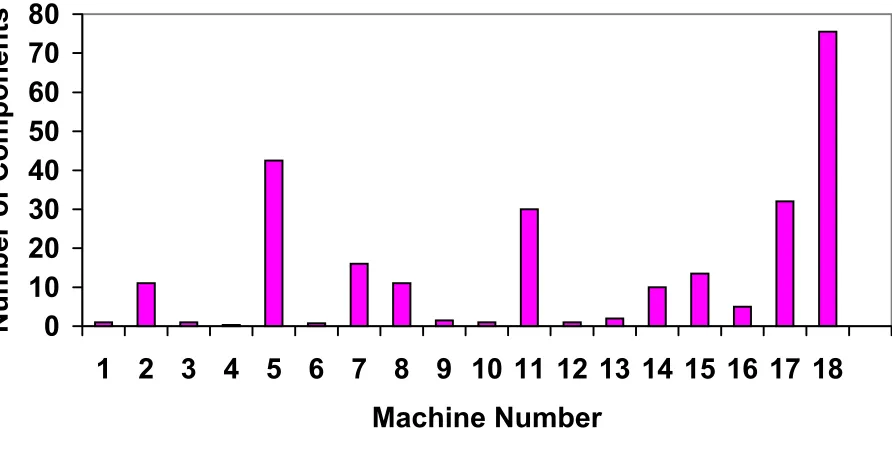
Number of machines available is more and they process very few components viz. IC turret lathe, Bench drill, etc. It is clear that the possibility of the formation of a cell with critical machines is abysmally low because of the very fact that they are associated with a large number of components. Since, Ideal machines process less number of components and their availability is good they lend themselves to efficient cell formation.Histogram for the categorization of machines is shown in Figure 1.
TABLE 2. Number of Components and Machines for WA-200 Project.
Machine
No. Name of the Machine No. of Machines No. of Components
1 IC turret lathe 1 1
2 H 22 lathe 3 33
3 HMT L 45 lathe 1 1
4 Bombay lathe 3 1
5 Radial drilling 2 85
6 Bench drill 4 3
7 Circular saw 1 16
8 Horizontal bandsaw 1 11
9 Milling FN 2H 2 3
10 Milling FN 3H 1 1
11 Vertical milling 1 30
12 Pedestal grinder 2 2
13 Centering machine 1 2
14 Facing & Centering 1 10
15 AF7 Boring 2 27
16 WMF Boring 1 5
17 Layout 2 64
18 Bench 2 151
19 A211 Boring 1 1
20 Thread chasing m/c 1 1
TABLE 3. Categorization of Machines
Categorization Machines
The classification is to an extent left to intuition, though a histogram of the number of machines available and the number of components that are processed by it greatly aids in this classification. To plot this histogram we convert the number of components processed by the machine as if only one of its kinds were available (similar to number
of components per machine) and then take the histogram. The categorization made from the histogram is shown in Table 3.
Step 4
Obtain initial solution (Machine Cells): Group the machines with highest similarity coefficient from the ideal machines group. Machines 7 and 2 are having similarity coefficient of 0.93, machines 14 and 2 are having similarity coefficient of 1.0 and machines 14 and 7 are having a similarity coefficient of 1.0 (similarity coefficient table not shown). Hence, group these machines in one cell. Machines 15, 8 and 3 are having zero similarity coefficient with each other and hence, they are put in different cells. Call this solution as Core cell. Core cell is shown in Figure 2 (a).Now, repeat the same procedure by adding non-critical machines from Table 3 to the core cell. Call this solution as revised solution. This is shown in Figure 2 (b).
Now, once again revise the solution by adding critical machines from Table 3 to the revised solution shown in Figure 2 (b). Call this as basic solution. This is shown in Figure 2 (c).
0
10
20
30
40
50
60
70
80
1 2 3 4 5 6 7 8 9 10 11 12 13 14 15 16 17 18
Machine Number
Number of Components
Figure 1. Histogram for categorization of machines.
2,7,14 15 8 3
(a)
2,7,14,1,4 15,10 8,20,12,13 3,6,9,16,19
(b)
2,7,14,1,4 15,10,11 8,20,12,13 3,5,6,9,16,19
(c)
Note that in the initial solution (Figure 2 (c)) we have considered only one machine of each type, though more than one machine is available for a few types of machines like Radial drilling machine, Milling machine FN 2Hetc (refer Table 3). These additional machines are assigned to the initial solution obtained and additional machines are duplicated wherever required. While assigning additional machines to the cell(s), we treated the problem as if the machine is being duplicated. This is to justify the assigning of the machine(s) into different cell(s). If the assigning of additional machine(s) is not justified, then we can make use of the same machine(s) available for other projects the company is undertaking. This is shown in step 6.
Step 5
Formation of Part family: We can
make use of Equation 1 with slight
modification for part family (jobs having
similar manufacturing attributes and processed
in common cell) formation as well. It results in
similarity coefficient matrix of the size 144
×
144 (number of components). Analyzing such
a big matrix for efficient part family formation
would be an impossible task. For part family
formation uses the following procedure.
Assign points to each component using the formula
)
x
(
p
x
i j ii
=
×
µ
(2)where µi = frequency of operations in the ith part family
xi = number of operations in ith cell
pj(xi) = probability of operations in the jth job nj = number of operations in a job
Assign components to that part family where it has scored highest point.
After applying Equation 2 the number machines and components associated with each cell is shown in Table 4.
Step 6
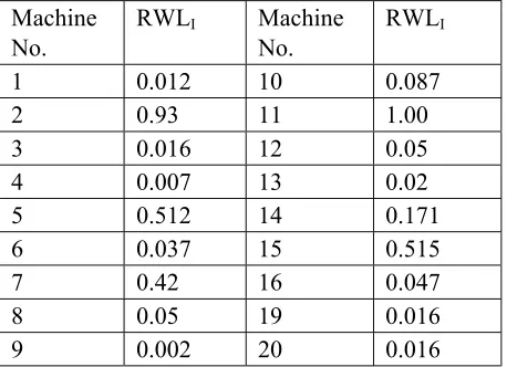
Compute Workload Index and duplicate additional machines based on workload index and cost parameters.Workload index for machine I (WLI) is calculated using the formula:
available
hours
of
Number
engaged
is
machine
which
for
hours
machine
of
Number
WL
index
load
Work
1
=
=
(3)
Company works 2 shifts a day (16 hrs.) and 300 working days a year.
WLI greater than ‘1’ implies that the machine is associated with larger processing times or number of machines available is insufficient. If WLI is less than ‘1’, it implies machine is underutilized. If WLI = 1 then machine is utilized for 100% of its efficiency. The limitation of workload index is that the index can vary from anything slightly greater than ‘0’ to very large number (theoretically speaking infinitely large). By dint of this, it is not possible to ascertain as to w h i c h ma c h i n e i s t o b e c o n s i d e r e d f o r duplication. To overcome this problem Relative workload index is calculated. Relative workload index of Ith machine (RWLI) is calculated using TABLE 4. Part Family for WA-200 Project.
Cell number 1 2 3 4
No. of m/c’s 5 3 4 6 No. of comp. 35 29 35 45
TABLE 5. Relative Workload Index for Different Machines.
Machine No.
RWLI Machine No.
RWLI
1 0.012 10 0.087
2 0.93 11 1.00
3 0.016 12 0.05
4 0.007 13 0.02
5 0.512 14 0.171
6 0.037 15 0.515
7 0.42 16 0.047
8 0.05 19 0.016
the relation
index
workload
Maximum
I
machine
of
index
Workload
RWL
index
load
Work
lative
Re
=
1=
(4)
Relative workload index lies between 0 and 1. Relative workload index for different machines is shown in Table 5.
To decide about the machines to be duplicated use the following procedure
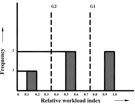
(a) Plot a graph of relative workload index (x-axis) vs. frequency of occurrence (y-(x-axis) as shown in Figure 3.
(b) Identify gaps (G1,G2,…,Gn) that segregate various block of workload index. If gap G1 is chosen, it implies machines having workload index greater than 0.8 (refer Figure 3) shall only be duplicated. One can consider the gap G2 also. But, this requires more investment than earlier case as more number of machines is considered for duplication (discussed in the latter part of the paper).
(c) List all the machines considered for duplication.
(d) Now, calculate cost workload index for machines, which are considered for duplication using the equation
s int Po RWL
CWLI = I × (5)
The ‘points’ in Equation 5 depends upon the cost of the machine. Table 6 shows costs of bottleneck machines (machines associated with many exceptional components) and their expected life.
‘Points’ in Equation 5 are determined by cost of the machine and slab points. It is shown in Table 7. Points given in Table 7 may vary depending upon range of costs of the machine(s) involved, budgetary constraint and number of machines short-listed for duplication. From the Table 7 it is clear that greater the cost of the machine, lesser will be its chances for duplication.
(e) Arrange all machines in ascending order of cost workload index.
0 0.1 0.2 0.3 0.4 0.5 0.6 0.7 0.8 0.9 1.0 1
2
G2 G1
Relative workload index
Fr
equen
cy
Figure 3. Frequency vs relative workload index.
TABLE 6. Cost details of Different Bottleneck Machines.
M/C No.
Name of the m/c
Cost (Rs. Lac)
Life(yrs.) 1 IC turret lathe 3.85 10
2 H22 lathe 2.5 10
5 Radial drilling 4.15 10
7 Circular saw 0.5 5
9 Milling FN2H 2.6 7
11 Vertical
milling 1.8 10
13 Centering machine 0.3 5 14 Facing and Centering 1.5 4
15 AF7 Boring 2.35 10
TABLE 7. Table for Assigning Points for Machines.
Cost of the machine (Rs.) Points
<= 1,00,000 7
1,00,000 < cost <= 2,00,000 5 2,00,000 < cost <= 3,00,000 4 3,00,000 < cost <= 4,00,000 3
(f) Chose Ith machine for duplication if it satisfy the criterion
×
θ
≥
∑
= k
1 I
I
I
CWL
CWL
(6)where k = number of machines considered for duplication. θ is a constant which ranges from 0.2 – 0.4 and depends on the budgetary constraints. Lower the θ, the larger the number of machines considered for duplication. It should be noted here that all the machines, which qualify this criteria, need not be duplicated. Final duplication of the machines is decided by the factors such as budgetary constraint, number of exceptional components processed by the machine, machine utilization and workload after duplication.
This step is emphasized in more detail in processing the exceptional components.
Step 7
Process exceptional componentsNevertheless the exceptional component, which required to be processed in more than one cell often, makes the task of engineers difficult and the solution to formation of cells become nontrivial. To realize the complete benefits of Cellular Manufacturing, it is imperative to have minimum or if possible zero exceptional components. Because, presence of exceptional component increases material handling, setup time, work-in-process inventory and make the job of scheduling more difficult and ultimately reduces productivity. But in real life situations we can find completely independent cells only in illustrative examples. Many algorithms proposed in the available literature for processing exceptional components assume that cell formation is already done. Exceptional components can be eliminated by duplicating the bottleneck machines (machines associated with many exceptional components), subcontracting the part, changing manufacturing process, redesigning the part, forming remainder cell (cell dedicated to the manufacture of exceptional components only). Owing to some extraneous reasons, the organization has not considered the option of sub-contracting the part. Changing manufacturing process or redesigning the part requires substantial investment, involves
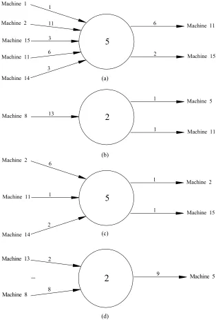
obsolescence of existing machineries, equipments and is a time consuming process. Hence these options were also not considered. We opted for eliminating the exceptional components by duplicating the bottleneck machines considering workload, cost, its associativity with exceptional components and justification for investment. From the basic solution obtained above (Figure 2 (c)) 45 components were found to be exceptional out of 144 components. Batch quantity for these exceptional components varied between 200-800. Among 45 exceptional components 8 components required processing in 3 cells and 37 components required processing in 2 cells. For duplication and/or assignment of additional machines into cells our major emphasis was to consider workload, its associativity with exceptional components, limitations of budgetary constraints and justification for investment. It should be noted that facilities 17, 18 (Layout and Bench) are required by all the cells and hence, it was decided to keep these facilities as common facility (Refer Figure 5).
Considering Workload
Select the gap G1 in Figure 3 for duplication. There are only 2 machines (2 and 11) in this category, which has very high relative workload index (0.93 and 1 respectively). Considering gap G1, we calculate cost workload index for machines 2 and 11 using Equation 5.72 . 3 4 93 . 0 2
CWLI = × = and CWLI11=1×5=5.
Choosing θ = 0.3 in Equation 6 we find both machines qualify for duplication.
Repeating the same procedure in gap G2 (machines 5, 7, and 15), machines that qualify for duplication are 7 and 15.
Hence, machines, qualified on the basis of workload index for duplication, are 2, 7, 11 and 15. Final decision on duplication of these machines will be made considering the associativity of these machines with exceptional components and justification for duplication.
exceptional components that flow between them. In Figure 4 the number in the circle represents the machine under consideration. The arrows pointing towards it are indicators of the machines that contribute exceptional components to the machine under consideration. The outward arrows show the machines to which the machine under
consideration contributes exceptional components. The machine numbers are written at the start or end of the arrow and the frequencies are written along the arrow. Machines identified as bottleneck are shown in Table 6. It should be noted that all the machines, which qualified for duplication based on workload index criteria are all listed in Table 6.
6
3 11 1
6
2 Machine 1
Machine 2
Machine 15
Machine 11
Machine 14
Machine 11
Machine 15
5
3
Fi
4 ( )
1 1
13
2
Machine 11 Machine 5
Machine 8
1 1 6
2
Fi
4 ( )
1
5
Machine 15 Machine 2
Machine 14 Machine 11 Machine 2
9 2
8
2
Machine 5Machine 8 Machine 13
Figure 4. Diagrammatic representation of exceptional component. (c)
(d) (a)
Justification for
Duplication Duplication of machine(s) is an important decision that an organization has to take. The reason is, it calls for investment and in the long run, significant savings in material handling costs resulting from decreased intercellular movements need to be realized. Various factors that need to be considered while duplicating the machine(s) include cost of the machine, its associability with exceptional components, and reduction in intercellular moves after duplication etc. In the present work cash flow (CF) is being considered for justifying the investment made. Among the different alternatives available for calculating cash flows Net Present Value (NPV), Benefit Cost Ratio (BCR) and Net Benefit Cost Ratio (NBCR) has been made use of. Brief outline of the criteria considered is discussed here.The Net Present Value rule states that ‘an alternative should be adopted only if the present value of the cash flow generated in the future exceeds its cost’. NPV is the net profit that accrues to the firm from adopting the investment. Assuming a constant cash flow Net Present Value is given by
(
CRF
,
CC
,
n
)
I
CF
NPV
=
×
−
(7)where:
CF = Cash Flow
CRF = Capital Recovery Factor CC = Cost of Capital
n = Number of years
I = Initial Investment Required
The values of CRF for a particular CC and n are obtained from the table of interest factors [7]. Benefit Cost Ratio measures the present value/rupee of outlay, it is considered to be a useful criterion for ranking a set of alternatives in the decreasing use of capital. The Benefit cost ratio or the profitability index is given by
(
CRF
,
CC
,
n
)
I
CF
BCR
=
×
(8)A variant of the benefit cost ratio is the Net Benefit Cost Ratio and is given by
I
NPV
NBCR
=
(9)A machine is not considered for duplication if NPV<0, or BCR<1 or NBCR<1. In any case, if the value of NPV, BCR and NBCR criteria is satisfied for more than one machine while eliminating exceptional component than the machine(s) with higher value of NPV, BCR, NBCR and which satisfy the budgetary constraints will be chosen. We calculate the cash flow (CF) for our calculations using the equation
(
)
(
)
(
Total
cos
t
of
moveing
the
part
)
components
of
.
No
movements
ercellular
int
of
Number
CF
×
×
=
(10) The data required for calculating the cost of
moving the part (not shown) was obtained from Industrial Engineering Department.
Alternatives for the Elimination of
Exceptional Components
Looking into the Figure 4a we can see that machines 5 and 11 are bottleneck machines. Considering this we have the option1. Duplicate machine 5 in cell 2 2. Duplicate machine 11 in cell 4
Considering the 1st option, i.e. duplicating machine 5 in cell 2, we calculate NPV, BCR and NBCR to justify the investment.
Using the equation of CF we get, CF = 21×200×10 = Rs.42,000
From the table of interest factors [15], we find that CRF = 6.1446 for a cost of capital of 10% (CC) and 10 years (n). Using the equations of NPV, BCR and NBCR, we get NPV= -156926, BCR = 0.622 and NBCR = -0.378. Since, NPV is negative, BCR less than one and NBCR is less than zero, duplicating machine 5 is not justified. It can also be recalled that the machine 5 did not qualify for duplication based on cost workload index criteria.
this type. It belongs to cell 1 (Refer Figure 4b). It is a bottleneck machine as it is having intercell movements with cells 2, 3 and 4. We can consider assigning of these additional machines to cells 2 and 3.
By duplicating machine 2 in cell 2 only one intercellular movement is reduced (Figure 4b). Hence, its cash flow will be only Rs.2000 (1×200×10). Using the equations of NPV, BCR and NBCR we get, NPV = -237710.8, BCR = 0.05 and NBCR = -0.951. Hence, assigning machine 2 in cell 2 is not justified. Considering assigning machine 2 to cell 3 we get CF = Rs.26,000
(13×200×10), NPV = -90240.4, BCR = 0.64 and NBCR = -0.361 and hence this option is also not justified.
The same procedure has been followed for all bottleneck machines and machines, which qualified on the basis of workload index criteria. Alternatives that justified the investment include duplicating machine 11 in cell 4 and machines 8, 13 in cell 1. Total costs of all these machines are within the budget constraint put by the company (Rs. 4 lacs). Forming remainder cell (cell dedicated to the manufacture of exceptional components only) is also considered for processing exceptional
11 cm
Cell 1
Cell 4
10 cm
16 13
9 cm 8 Common 6
8 cm 14 4 9 5 3
11
7 cm
1 2 7
17
18 19
6 cm
5 cm
Passage Passage Passage
8
4 cm 11
3 cm Cell3 13
17
18 15
2 cm 12 10
20 Commo
n
1 cm Cell 2
0.5 1 1.5 2 2.5 3 3.5 4 4.5 5 5.5 6 6.5 7 7.5 8
1 cm 2 cm 3 cm 4 cm 5cm 6 cm 7 cm 8 cm
Scale X-Axis: 1cm = 5m Each cell is 0.25cm X 0.25cm
components. Machines considered for the formation of remainder cell were 1,2,5,7,8,9,11,14 and 15. Repeating the same procedure we get NPV = 1156326, BCR = 0.3946 and NBCR = -0.605. Hence, this option is not feasible.
Step 8
Arrange cells and machines within the cell: For arranging cells and for arranging machines within the cell we have used from/to chart analysis. This includes the following steps: (a) Develop the from-to-chart from part routingdata. Machines 17, 18 (bench and layout) facilities are required commonly by all the machines and hence are not used for from-to-chart calculation.
(b) Determine the to/from (T/F) ratio for each machine (not shown).
Arrange cells/machines in order of increasing to/from ratio (not shown). The notion is that cells/machines that have a low to/from ratio receive work from other cells/machines but distribute work to other cells/machines. Cells and machines within the cells were arranged in accordance with to/from ratio obtained. Final layout obtained by the proposed method is shown in Figure 5.
Material movement when traced through string diagram revealed that there would be drastic reduction in material handling, if the components were processed through Cellular layout. With the present layout total material movement is 3148.2 meters and through proposed layout it was found to be 1836.5 meters.
4. CONCLUSIONS
The paper presented is an integrated approach for cell design. Cell formation dealt in this paper is progressive i.e. it considers non-critical, ideal and critical machines individually. In real life situations this approach increases the scope for efficient machine cell formation and reduces the complexity of the problem. Though many cell formation techniques are available in the literature either they are not tested for practical applications
or though authors claim that their methods have been applied successfully, details of their implementation are not disclosed. Formation of machine cells, part family, processing of exceptional components and designing of layout is being dealt systematically. In most of the literature available authors treat the problem of Cellular Manufacturing as the problem of formation of machine cells and part families. This paper presents an integrated approach for cell formation, processing of exceptional components and arrangement of Cellular layout. The paper presented considers workload on each machine and cost before duplication. A total reduction of about 58% could be achieved in material handling by implementing the proposed method. Other benefits of Cellular Manufacturing such as reduced work-in-progress inventory, setup time etc. can be realized after the implementation of Cellular Manufacturing.
5. REFERENCES
1. Srinivasan, G., “A Clustering Algorithm for Machine Cell Formation in Group Technology Using Minimum Spanning Trees”, International Journal for Production Research, Vol. 32, No. 9, (1994), 2149-2158.
2. Crama, Y. and Oosten, “Models for Machine-Part Grouping in Cellular Manufacturing”, International Journal for Production Research, Vol. 34, No. 6, (1996), 1693-1714.
3. Jayakrishnan, N. G. and Narendran, T. T., “On the Use of the Asymptotic Forms of the Boolean Matrix for Designing Cellular Manufacturing Systems- an Improved Approach”, European Journal of Operations Research, Vol. 100, (1997), 429-440.
4. McAuley, J., “Machine Grouping for Efficient Production”, Production Engineer, (1972), 53-57.
5. Waghodekar, P. H. and Sahu, S., “Machine Component Cell Formation in Group Technology: MACE”, International Journal for Production Research, Vol. 22, No. 6, (1984), 937-948.
6. Parashar, N. and S., “A Heuristic Approach to Machine Cell and Part Family Formation in Group Technology”, Industrial Engineering Journal, Vol. 24, No. 2, (February 2000), 2-7.