Application of Game Theory on Inventory Level Decision Making

Published online November 25, 2014 (http://www.sciencepublishinggroup.com/j/ijber) doi: 10.11648/j.ijber.20140306.12

ISSN: 2328-7543 (Print); ISSN: 2328-756X (Online)

Application of game theory on Inventory level decision

making

Masoud Vaziri

*

, Manbir Sodhi

Dept. of Industrial and Systems Engineering, University of Rhode Island, Kingston, USA

Email address:

[email protected] (M. Vaziri), [email protected] (M. Sodhi)

To cite this article:

Masoud Vaziri, Manbir Sodhi. Application of Game Theory on Inventory Level Decision Making. International Journal of Business and Economics Research. Vol. 3, No. 6, 2014, pp. 211-219. doi: 10.11648/j.ijber.20140306.12

Abstract:

Many companies producing durable products, profit more from spares than the base parts. In a competitive and uncertain aftermarket, an Original Equipment Manufacturer (OEM) can benefit from Game Theory to manage spare parts inventories. We study the spare parts inventory game as an N-person non-zero-sum single-shot game where players play simultaneously. The game is restricted to a two-player (the OEM and the market) non-cooperative game setup. The market is an unreasoning entity whose strategic choices affect the payoff of the OEM, with no interest in the outcome of the game. This is a game against nature, which means the OEM plays against the market. The OEM decides on a pricing strategy (in a competitive manner with low cost manufacturers or will-fitters to absorb more customers) and the order-up-to stock level, and its inventory level strategy is not dominated – i.e. the game has a mixed strategy solution. This solution maximizes the payoff for the OEM by setting the price and the inventory level based on assumptions on the lower and upper bounds of the demand’s distribution parameters.

Keywords:

Spare Parts Management, Spare Parts Pricing, Game against Nature, Stochastic Demand

1. Introduction

The spare part business involves purchasing, warehousing, selling and delivering of spare parts to customers. It is common to include extended activities such as customer services and warranty issues within the definition of the spare part business [1]. For many companies producing durable products, spare parts are the most profitable function of the corporation [2]. Despite an absence of reliable data, researchers believe that the spare parts business is very profitable, and spare parts contribute to one-third of the net sales and two-third of the profits [1]. The size of aftermarkets in industries such as automobiles, white goods, industrial machinery, and information technology is four to five times larger than the original equipment businesses. In 2006, the of spare parts and after-sales services in the United States at 8% of annual gross domestic product (GDP), that means American customers spend about 1 trillion US dollars annually on assets they already own [3]. In 2010, according Rolls-Royce group annual report, Rolls-Royce engine-maker generated more than half of its revenue (more than 5.5 billion British pounds) from these service activities. The share of a company’s spare parts revenue is an indicator of the

importance of the spare parts business. In a case study for different firms, on the average companies generate 13.3% of their revenues from the sale of spare parts [2]. In the automotive industry, the profit margins from spare parts sales are three to four times higher than the margins from car sales. Some firms sell their primary products (i.e. machines) with the price close to the production cost with the goal of attracting future demand for spare parts [4]. In 2005, the size of aftermarket goods and services (in a broad aggregation including replacement of toner cartridges to engines of cruise ships) was 400 billion US dollars and recently this amount grown to 700 billion US dollars [5].

cases the nature of demand is intermittent and forecasting methods can predict demands. Several factors differentiate spare parts inventories from other types of inventories. The main factor is customers’ expectation regarding quality of services. The following factors can significantly affect the customers’ expectation [6-9]:

Delays in repairing;

Spare parts demand (which mostly is intermittent); High risk of obsolescence due to complexity of products and their life cycles;

The life cycle of the spare parts is affected by finished goods life cycle. Their life cycle can be divided into three phases: initial, normal or repetitive and final [10]. Therefore, demands for spare parts depend on finished goods, and the following factors affect the demand [11]:

Size and age of the final products (sales, running fleet, installation base, etc.);

Products maintenance characteristics (preventive, corrective, etc.);

Parts characteristics and their defects (wear, accident, aging, etc.);

Spare parts inventory management deals with an uncertain demand for spares and the competitive market. Therefore, Game Theory can be useful to address spare parts inventory problems. The first application of Game Theory, cooperative and non-cooperative games, goes back to [12]. Supply chain management has both cooperative and non-cooperative interactions between different agents, and the cooperative games in the supply chain management are called inventory games. It is common to categorize cooperative games into deterministic and stochastic games using through EOQ and Newsvendor policies respectively [13]. The EOQ model is designed for multi-item orders and known as the joint replenishment game. The latter game is based on the classic-News Vendor policy and is known as the Newsvendor centralization game. Both games have infinite repetition and are used for single-stage and stationary problems.

In [14], the authors provide an extensive survey of supply chain games which looks for the existence and uniqueness of the equilibrium in non-cooperative games. However, they develop different Game Theoretical techniques to study four types of games including:

non-cooperative static games; dynamic games;

cooperative games;

signaling, screening and Bayesian games;

[15] is one of the first representations of the EOQ game where the cooperation between different firms is structured, and the proportional division method is used for the cost allocation. In [16], an infinite-horizon deterministic problem has been developed, and it showed that this game has a non-empty core where optimal replenishment is determined by power-of-two policies. [17] studied inventory games and cost allocation with a base of EOQ models. Similarly, [18] uses this method for economic lot-size games. This method is applied to a scenario with a fixed time horizon, known demand for a single item and backlogging is not allowed.

A successful inventory control policy determines the inventory levels which are cost-optimal solutions. In inventory systems over-stocking leads to high cost of holding costs and under-stocking leads to backorder costs. Inventory systems consider these costs and introduce proper objective functions to minimize the cost of inventory. In most cases, backorder costs are difficult to estimate. Backorder costs can be as simple as penalty costs or severe, such as loss of business. There are three types of backorder costs [19]:

Penalty cost, in case of warm relation between business parts;

Lost business, in case of cool relation between business parts;

Combination of first two possibilities which means cool-warm relationship;

We consider the backorder cost as the warm relation, and backorder is modeled as a penalty cost in the cost function. In real world, spare parts are characterized as slow moving items with intermittent demand. The occasional demand arrivals for spare parts are interpreted by exponentially distributed inter-arrival times. Therefore, demand arrivals can be modeled as the Poisson process [20]. The continuous order-up-to level policy, also known as the base stock policy, is near-optimal and practical to implement for inventory systems for slow moving items such as spare parts that have demand arrivals with the Poisson process [21].

The number of spare parts is much larger than the primary products but the number of sale is low. When the number of spare parts sale is low, profit depends more on sale price compared to the amount of sale or reduction in production cost. Despite the low number of spare parts sale, they make up a considerable part of the manufacturers’ profits. For instance, a consumer durable product company can increase its profit by 30% with only 2.5% average increase in the products price and an industrial equipment manufacturer benefits from the 35% increase in its profit by increasing its price level by only 3%. Therefore, the price of the spare parts is the main factor to increase the manufacturers’ profit margin. Also, consistent pricing will result in greater customer satisfaction and loyalty. Three major activities improve the competitiveness of a company: the decrease of cost; the increase of market share and the price adjustment known as a pricing strategy. Moreover, in the aftermarket business, in addition to the OEM, there are other low cost manufacturers, known as will-fitters, who supply spare parts and compete with the OEM. The price of the parts has a significant effect in the distribution of the market share between the OEM and its competitors. In other words, the OEM sale price is its decision variable that determines its demand share in the aftermarket.

solution of the game maximizes the profit of the OEM in the buyer-seller environment. The remainder of the paper is organized as follows. Section 2 describes the proposed spare parts inventory game and presents the notation used in the paper. The market demand, the OEM expected cost function, the game setup and the solution of the mixed-strategy are derived subsequently. In section 3, we present the assumptions and the results of the numerical study, followed by related simulation results in section 4. We end in section 5 with conclusions.

2. Inventory Game, Game against Nature

Supply chain management and inventory management can benefit from Game Theory. In general, Game Theory can improve or clarify interactions between different groups who are competing against each other. Cooperative and non-cooperative games are used to model several supply chains with single and multi-period settings [22].

In the context of supply chains, Game Theory can be used for decision-making when there are conflicts between multiple entities. For instance it has been used to analyze detailed supply chains [14] where cooperative and non-cooperative games are used to solve static and dynamic games. The majority of studies focus on the existence of the equilibrium in non-cooperative game.

The goal of this paper is to investigate the spare part inventory game as an N-person non-zero sum single-shot game where players play simultaneously. In order to achieve this goal, the problem is restricted to a two-person, non-cooperative game setup. The game has two players; the OEM and the market. The game has been set up from the OEM perspective, which means the solution of the game results in maximum payoff or minimum loss for the OEM.

Game Theory is the logical analysis of situations of conflicts and cooperation, and can be used in situations can be used in situations where [23]:

There are at least two players;

Each player has a number of possible strategies; The strategies chosen by each player determine the outcome of the game;

Associated with each possible outcome of the game is a collection of numerical payoffs, one to each player; Game Theory studies how the player should play rationally, which implies that players select their strategies on action that result in maximum profit. The selected strategy pair is known as a Nash Equilibrium of the game. In this paper, we assume that the game is a non-cooperative game and the market is unkind and chooses hostile strategies. The OEM knows the demands for spare parts arrive as a non-stationary Poisson process, but is not aware of the exact distribution of the intensity factors and can only forecast the bounds of the intensity factors. Also, the OEM sale price with comparison to the will-fitters sale prices has an influence on the demand intensity factors which is estimated by the OEM.

We consider the market as an unreasoning entity whose strategic choices affect the payoff the manufacturers, but

which has no interest in the outcome of the game. The aforementioned characteristic of the market enables us to consider the spare parts inventory game as a game against nature. Our literature review including: [13], [15], [19], [22] shows us, none of the research has been dedicated to the application of the game against nature in the spare parts inventory management. One of the recent studies related to the application of the game against nature in the strategic decision-making is provided by [24]. The author discussed the psychological aspect of decision-making in games against nature where the selected strategies improve the effects of Minimax strategies in the cases of risk-aversion. In our study we model the spare parts inventory management as a game against nature which means the OEM competes with will-fitters on the sale prices meanwhile play against the market to optimize its spare part inventory level.

2.1. The Market Demand

Spare parts demand is often intermittent or lumpy which means long variable periods without any demand are frequent. When demand occurs and cannot be met, high losses may occur. Demand forecasting methods can be used to plan inventory. [26] Introduced a classical method for demand forecasting and [27] has provided a related literature review covering work over the last fifty years.

In this paper we assume that the OEM has limited information about the market’s expected demand. The OEM knows that demands for spare parts arrive as a non-stationary Poisson process , i.e. the rate of the process changes with time, but the exact distribution of these factors over the time is not observed and only the upper and lower bounds of the intensity factors are forecasted.

In the aftermarket business, other than the OEM as an original manufacturer, there are other low cost manufacturers, known as will-fitters, who can manufacture the same parts and deliver them to the market. Based on the sale price of the manufacturers, the market share for spare parts will be allocated among suppliers. In other words, manufacturers compete with each other on their sale prices to absorb more customers, so the sale price is a decision variable for the OEM to optimize payoff in the aftermarket.

Because of the intermittent and slow moving characteristics of spare parts demand, we consider it to be a Poisson process. A Poisson process with an intensity factor or rate of λ is a stochastic process in which the inter-arrival time distribution is exponential with mean time of μ = 1/λ and the arrival distribution is Poisson with the rate of λ . If λ is constant over time, the process is a stationary Poisson process and when λ changes over time, the process is a non-stationary Poisson process. In the case of spare parts management, the rate of demand depends on three factors:

λ

Upper

λ

Lower

Figure 1. Demand for spare parts distribution during product life span modified from [28]

These factors are not constant over time. Intuitively, we can assume that the demands are a non-stationary Poisson process in which the demand rate is a function of time λ t .

In this study, we assume that the OEM introduces a new product to the market and wants to forecast demands for spare parts in the next period. The OEM considers two major phases when parts fail: the initial phase (introduction phase) and the repetitive phase (growth, maturity and decline phase). Figure 1 graphs number of products in the market and demand for the spare parts during the product life span for automotive electronics industry [28].

Demands for spare parts arrive as a non-stationary Poisson process with two levels of intensity factors:

Upper bound intensity factor λ : The repetitive phase of the original parts consists of the period right before the end of the original production and post product life cycle as the repetitive support, which has higher failure intensity;

Lower bound intensity factor λ : The initial phase of the original parts consists of the period right after the introduction of the original products to the market as the initial support, which has lower failure intensity; Regarding the competition among the OEM and will-fitters, sale prices can affect the allocation of spare parts demand among the manufacturers. We assume that the manufacturers are capable of forecasting the demand intensity factors with respect to their sale prices. Based on the sale prices, the upper bound and lower bound intensity factors are known by the OEM which are listed in Table 1:

Table 1. The market demand parameters

Spare Part Sale Price Upper Bound Rate Lower Bound Rate

c λ λ

2.2.The OEM Cost Function

The OEM must determine the sale price and the spare parts stock level in the order-up-to level inventory policy. The payoff for OEM is the profit of the OEM K which is the

difference between the cost of production and inventory K and the revenue K attained by selling spare parts.

Table 2. Required parameters to calculate cost of production and inventory.

Notation Parameter definition

D Demand (in units per period)

S Spare parts inventory level (in units)

c Variable cost of production (in dollars per unit) p Penalty cost (in dollars per unit per period) h Holding cost (in dollars per unit per period) c Sale price (in dollars per unit)

Let (X) be a random variable and Pr{X=x} determines the probability that the random variable (X) takes on a specific value x from some unspecified probability distribution.

E[X] = ∑' x Pr {X = x}

()* (1)

The expected value is E[X] that is given by Equation (1). As it was mentioned in the last section, we assume that the demand arrives as a Poisson process. The Poisson distribution is given by Equation (2):

p x = +,- ./0_(! (2)

Where the mean E[X], from (1) is found to be (λT . It is assumed that λ is the average annual demand for spare parts or the intensity factor and (T) is the average lead time measured in years. The origin of the single-item inventory theory is in [29]. If the demand for an item is a Poisson process with an intensity factor of λ and if the lead time for each failed unit is independently and identically distributed according to any distribution with mean (T) years, then the steady-state probability distribution of the number of failure units in the lead time has a Poisson distribution with mean (λT . The most common inventory policy for low demand, high cost repairable items is the order-up-to level inventory policy which is a one-for-one policy with a stock level of (S) and re-order point of (S-1). There are two principal measures of item performance including: the fill rate, the percentage of demands that can be met at the time they are placed, and the backorders, the number of unfilled demands that exist at a point in time. The expected fill rate (EFR) and the expected number of backorders (EBO) are non-negative quantities and they are calculated as:

EFR S = ∑56*Pr{X = x}

()7 (3) EBO S = ∑' x − S Pr {X = x}

()5;* (4)

Moreover, the expected number of parts in inventory is derived as:

EI S = ∑5 S − x Pr {X = x}

()7 (5)

us the cost of production and inventory:

K = c × S + p × EBO S + h × EI S (6)

Equation (7) gives us the revenue of selling products:

K = c × D × EFR S (7) Equation (8) gives us the OEM’s payoff:

K = K − K (8) The cost of the production and inventory, and the revenue of selling products are functions of the sale price and inventory levels, which are the strategic actions of the OEM. The required parameters to calculate the OEM’s cost and payoff, which are used in (6) and (7), are listed in Table 2.

2.3.The Game Setup

In this scenario, players choose their strategies simultaneously and the game is a static game that can be modeled and solved by finding Nash Equilibrium. This configuration requires the following protocol:

Players play simultaneously;

The OEM possesses the information of the original parts failure rates and can predict the allocated demand rates including: the upper bound intensity factor

λ and the lower bound intensity factor

λ with respect to its selected sale price;

The market as a nature has two choices of Poisson process demand types with upper and lower bounds intensity factors;

The probability that the market plays with lower bound demand is (P) or P MarketCDEFGH _;

Respectively the probability that the market plays with upper bound demand would be (1-P);

The OEM has several strategies which are order-up-to inventory levels (as discrete numbers) that varies from 1 to N;

Table 3. The payoff matrix of inventory game

Market (Nature)

OEM

Order-up-to level Dlower Dupper

S1 KB(S1,Dlower) KB(S1,Dupper)

⋮ ⋮ ⋮

SN KB(SN,Dlower) KB(SN,Dupper)

The game setup can be shown in strategic or matrix form. Table 3 gives us the information of the game setup in the matrix form. This matrix known as the payoff matrix and the value of each cell is the payoff the OEM. Regarding the probability of market decision-making P MarketCDEFGH _{, the}

expected utility (EU) of the OEM will be calculated from (9) where (i) is order-up-to stock levels that varies from 1 to N:

E OEMJ _{= P Market}CDEFGH × K OEMJ, MarketCDEFGH +

P MarketCLMMGH _{× K OEM}J_{, Market}CLMMGH ₍₉₎

Equation (10) tells us that the total probability of market decision-makings equals to 1.

P MarketCDEFGH + P MarketCLMMGH = 1 ₍₁₀₎

The investigation of the payoff matrix declares that there is no dominant strategy in this game. In other words, the lack of dominant strategy leads to the lack of pure strategy, implying the optimal solution depends on the probability of the market’s demand.

2.4.Mixed Strategy Solution

In the theory of games, a game has a mixed strategy solution where a player has to choose his/her strategies over available sets of available actions randomly. A mixed strategy is a probability distribution that assigns to each available action a likelihood of being selected. In 1950, John Nash proved that each game (with a finite number of players and actions) has at least one equilibrium point known as Nash Equilibrium. This saddle point exists whenever there is a dominant strategy.

NK sJ

∗_{, D > K s} J , D K sJ∗, D > K sJ , D

∀ sJ& T

U (11)

In our game this can be explained based on the OEM payoff matrix where there is a specific level of inventory for the OEM that satisfies (11). In case of existence of this specific level of inventory, the selected inventory level would be the dominant strategy for the OEM.

In this decision-making problem, the OEM is making a choice between different alternatives. If the payoff for each alternative is known, the decision is made under certainty. If not, the decision is made under uncertainty. The solutions for decisions under uncertainty and risks optimize expected utility (EU) and subjective expected utility (SEU). Given a choice of X and n different possible payoffs in nature, SEU is calculated by multiplying the payoff for each option by the subjective probabilities. The decision maker chooses an action with the highest expected utility. The subjective expected utility (SEU) determines the inventory level for the OEM.

3. Results and Discussion

In order to demonstrate the decision-making of the OEM based on the implication of the game against nature and the mixed strategy solution, we consider a single-item spare part inventory game. The sample parameters of our spare parts management system are listed in Table 4. Also we assume that the average lead time (T) is one year.

Table 4. Parameters of the sample spare part inventory

Notation Parameter value

D Dlower: VWXYZ[& Dupper: V\]]Z[

S Decision variables (1 to 10)

c 40

p 60

h 5

3.1.Numerical Study

Table 5. Parameters of the sample spare part inventory

Spare Part Sale Price Upper Bound Rate Lower Bound Rate

90 5.5 3.5

100 5 3

110 4.5 2.5

120 4 2

130 3.5 1.5

As it was mentioned in previous sections, the OEM decision variables are the spare part order-up-to level and the sale price. Demand for spare parts arises when the original parts fail, then the emerging demand would be allocated among the OEM and will-fitters in the aftermarket business. The main factor that affects the allocation of the demand among the suppliers is the spare part sale price.

We assume that the OEM can forecast the demand bounds (including the lower bound intensity factor and the upper bound intensity factor) with respect to the spare part sale price.

In Table 5, the forecasted demand rates versus the spare part sale prices are depicted. At each sale price level, the expected utility of the OEM for 10 different levels of inventory as a function of the probability that the market chooses to play with the lower bound intensity factor in the aftermarket business

P MarketCDEFGH _{has been calculated. According to the}

results of the game against nature, the optimal decision variables of the OEM are determined. Table 6 shows the result of our spare part inventory game:

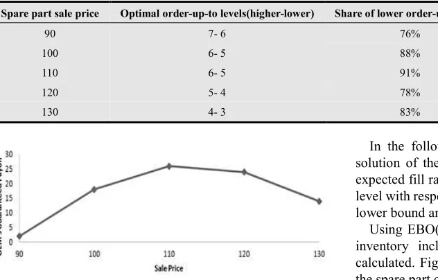
As we can see the Nash Equilibrium of the game is the Maximin strategy of the OEM that is acquired by choosing the best of the worst payoff. This strategy determines the OEM’s guaranteed payoff which reaches to its maximum level at the sale price of 110. In other words, the optimal sale price for the OEM is 110 and the optimal inventory policy is to keep the order-up-to level of the spare part inventory at 6 and 5 for the 9% and 91% times of the production horizon respectively. Figure 2 depicts the trend of the OEM’s guaranteed payoff versus the sale price. As it is shown, the maximum guaranteed payoff is achieved at sale price of 110.

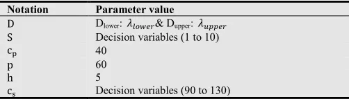
Table 6. Optimal spare part inventory levels

Spare part sale price Optimal order-up-to levels(higher-lower) Share of lower order-up-to level Guaranteed payoff Maximum payoff

90 7- 6 76% 2 59

100 6- 5 88% 18 90

110 6- 5 91% 26 115

120 5- 4 78% 24 127

130 4- 3 83% 14 130

Figure 2. The OEM’s guaranteed payoff vs. The sale price

In the following the detailed description of the optimal solution of the game is presented. In Table 7, the resulting expected fill rate, expected backorder and expected inventory level with respect to different values of the stock levels for the lower bound and upper bound of the demand are listed.

Using EBO(S), EI(S) and related stock levels, the cost of inventory including the holding and backorder costs is calculated. Figure 3 shows the OEM’s inventory cost versus the spare part order-up-to levels.

Table 7. Numerical example for a single-item inventory

Mean annual demand (λ) 2.5 4.5

Average lead-time (T) 1 1

Item cost (^_{_}) 40 40

S EFR(S) EBO(S) EI(S) EFR(S) EBO(S) EI(S)

0 0.00 2.50 0.00 0.00 4.50 0.00

1 0.08 1.58 0.08 0.01 3.51 0.01

2 0.29 0.87 0.37 0.06 2.57 0.07

3 0.54 0.41 0.91 0.17 1.75 0.25

4 0.76 0.17 1.67 0.34 1.09 0.59

5 0.89 0.06 2.56 0.53 0.62 1.12

6 0.96 0.02 3.52 0.70 0.32 1.82

7 0.99 0.01 4.51 0.83 0.15 2.65

8 1.00 0.00 5.50 0.91 0.07 3.57

9 1.00 0.00 6.50 0.96 0.03 4.53

Figure 3. The OEM’s inventory cost vs. the order-up-to level

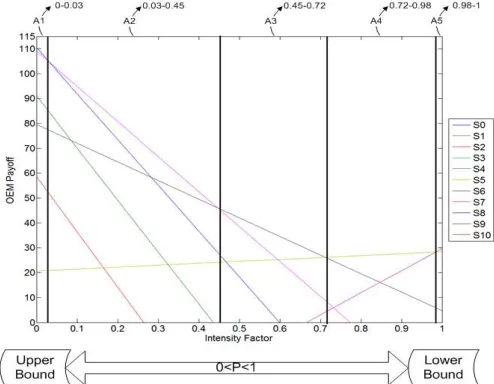
The expected utility of the OEM for 10 different levels of inventory as a function of the probability that the market chooses to play with the lower bound intensity factor in the aftermarket business P MarketCDEFGH _{has been calculated.}

The results are depicted in Figure 4 where the OEM payoff distribution is graphed vs. the probability of the lower bound intensity factor.

Figure 4. The OEM payoff distribution vs. the probability of the lower bound intensity factor

According to the results of the SEU, the optimal decision variables of the OEM are determined which maximizes the payoff in the aftermarket game. This decision-making is the inventory policy of the OEM that states the OEM should change the inventory level based on the probability of the market’s intensity factor or demand:

A1: If 0<P MarketCDEFGH _{<0.03 then select the}

inventory level of 8;

A2: If 0.03< P MarketCDEFGH _{<0.45 then select the}

inventory level of 7;

A3: If 0.45< P MarketCDEFGH _{<0.72 then select the}

inventory level of 6;

A4: If 0.72< P MarketCDEFGH _{<0.98 then select the}

inventory level of 5;

A5: If 0.98< P MarketCDEFGH _{<1.00 then select the}

inventory level of 4;

The lowest point in the upper envelope of the expected

payoff involves an inventory level of 6 and an inventory level of 5. According to the results of mixed strategy for that 2 × 2 matrix game, the optimal decision variables of the OEM are determined. The solution of the mixed strategy states that the OEM should switch between inventory levels of 6 and 5 with probability of 9% and 91% respectively. The resulting mixed strategy guarantees the payoff of 26 for the OEM in the long run.

On the other hand, the OEM has the opportunity to invest in performing a comprehensive market survey and precise data analysis to develop an accurate demand forecasting for the spare parts. Let us assume this investment costs the OEMC_{b cd eJfg}. The method provided in our study helps the OEM to decide whether investing in a more precise demand forecast is warranted. Equation (12) could evaluate the effort of the OEM to invest on extra demand forecasting. Once Equation (12) is satisfied, extra effort on demand forecasting is sensible:

Max K − GT K > Cb cd eJfg (12)

Where GT K is the result of the mixed strategy solution for the OEM’s payoff. In our proposed numerical study the

Max K is equal to 115 and GT K equals to 26. Therefore, as long as Cb cd eJfg is less than 89, extra effort on demand forecasting would be a rational activity.

3.2.Simulation

In order to examine the accuracy of the Game theoretical solution, a Monte Carlo simulation has been developed which relies on random sampling to obtain numerical results. The simulation runs many times to obtain the payoff of the OEM with respect to uncertainty of the market.

Figure 5. Simulation results – The OEM payoff vs. the probability of the lower bound intensity factor, General Policies &GT

The simulation follows the following particular pattern: 1 Defines a domain of possible inputs;

performing a deterministic computation over the inputs; 4 Aggregates the results;

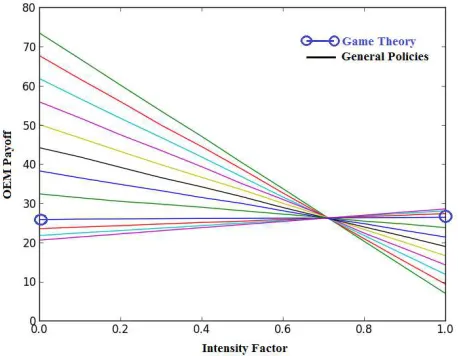
The goal of the simulation is to show the comparison of the Game Theory approach and any other inventory and production policy. In figure 5, the payoff of the OEM vs. the probability of the lower bound intensity factor while implementing Game Theory solution and some other inventory policies (General Policies; including different levels of order-up-to level inventory with different strategies of keeping inventory for example setting order-up-to level to 4 and 8 and switching among them with probability of 30% and 70% respectively and etc.) is depicted. As we can see Game Theory approach guarantees the payoff of 26 for the OEM by switching among order-up-to levels of 6 and 5 with probability of 9% and 91% respectively.

Figure 6. Simulation results - The OEM payoff vs. the probability of the lower bound intensity factor General Policies (identical levels with different strategies)&GT

The performance of the Game Theory approach is graphed in Figure 6 where general policies are considered as implementing order-up-to level of 5 and 6 with different strategies to keep the inventory such as 30% lower level and 70% upper level and etc. The results of the Monte Carlo simulation states that Game Theory approach allocates guaranteed payoff to the OEM in an uncertain market situation.

4. Conclusion

In this study, Game Theory is applied to determine the sale price and the spare part stock level for an OEM who manufactures single-item spare parts, keeps them in the inventory with order-up-to level inventory policy and sells them to the market. The spare parts inventory management is studied as an inventory game in case of an N-person non-zero sum single-shot game where players play simultaneously. In order to achieve this goal, the problem is restricted in two-person, non-cooperative game setup. The game has two players: the OEM and the market, and the game has been set up from the OEM’s perspective, which results in the maximum payoff or minimum loss. It has been assumed that

the game is a non-cooperative game and the market is unkind and chooses hostile strategies. The OEM can only forecast the upper and lower bounds of the market’s intensity factors. In the aftermarket business, other than the OEM as an original manufacturer, there are other low cost manufacturers, known as will-fitters, who can manufacture the same parts and deliver them to the market. Based on the sale price of the manufacturers, the total demand for the spare parts will be allocated among suppliers. In other words, manufacturers compete with each other on their sale prices to absorb more customers, so the sale price is a decision variable for the OEM to optimize its payoff in the aftermarket. The OEM possesses the information of the original parts failure rates and can predict the allocated demand rates including: the upper bound intensity factor and the lower bound intensity factor with respect to its selected sale price. The market is considered as an unreasoning entity whose strategic choices affect the payoff the OEM, but which has no interest in the outcome of the game. This is modeled as the game against nature which means the OEM plays against the market.

In our game there is no dominant level of inventory for the OEM i.e. the game has the mixed strategy solution. The solution of the mixed strategy, determines the strategies of the OEM to maximize the payoff in the aftermarket business. The OEM chooses the optimal level of inventory with respect to the probability of intensity factors that the market can produce. A comparison of the maximum attainable payoff and guaranteed payoff in the uncertain situation would justify the OEM’s extra investment on improving the demand forecasting efforts.

References

[1] P. Suomala, M. Sievänen, and J. Paranko, “The effects of customization on spare part business: a case study in the metal industry,” International Journal of Production Economics, vol. 79, no. 1, pp. 57–66, 2002.

[2] S. Wagner and E. Lindemann, “A case study-based analysis of spare parts management in the engineering industry,” Production Planning and Control, vol. 19, no. 4, pp. 397–407, 2008.

[3] M. A. Cohen, N. Agrawal, and V. Agrawal, “Winning in the aftermarket,” Harvard business review, vol. 84, no. 5, p. 129, 2006.

[4] M. J. Dennis and A. Kambil, “SERVICE MANAGEMENT: BUILDING PROFITS AFTER THE SALE.,” SUPPLY CHAIN MANAGEMENT REVIEW, V. 7, NO. 3 (JAN./FEB. 2003), P. 42-48: ILL, 2003.

[5] T. Gallagher, M. D. Mitchke, and M. C. Rogers, “Profiting from spare parts,” The McKinsey Quarterly, vol. 2, 2005. [6] M. A. Cohen and H. L. Lee, “Out of touch with customer

needs? Spare parts and after sales service,” Sloan management review, vol. 31, no. 2, pp. 55–66, 1990.

[8] J. A. Muckstadt, Analysis and algorithms for service parts supply chains. Springer, 2004.

[9] S. Kumar, Parts Management Models and Applications: A Supply Chain System Integration Perspective. Springer, 2004. [10] L. Fortuin, “The all-time requirement of spare parts for service

after sales—theoretical analysis and practical results,” International Journal of Operations \& Production Management, vol. 1, no. 1, pp. 59–70, 1980.

[11] L. Fortuin and H. Martin, “Control of service parts,” International Journal of Operations \& Production Management, vol. 19, no. 9, pp. 950–971, 1999.

[12] J. Von Neumann and O. Morgenstern, Theory of Games and Economic Behavior (Commemorative Edition). Princeton university press, 1953.

[13] M. Dror and B. C. Hartman, “Survey of cooperative inventory games and extensions,” Journal of the Operational Research Society, vol. 62, no. 4, pp. 565–580, 2010.

[14] G. P. Cachon and S. Netessine, “Game theory in supply chain analysis,” Tutorials in Operations Research: Models, Methods, and Applications for Innovative Decision Making, 2006. [15] A. Meca, J. Timmer, I. García-Jurado, and P. Borm,

“Inventory games,” European Journal of Operational Research, vol. 156, no. 1, pp. 127–139, 2004.

[16] S. Anily and M. Haviv, “The cost allocation problem for the first order interaction joint replenishment model,” Operations Research, vol. 55, no. 2, pp. 292–302, 2007.

[17] Dror and Hartman, “Shipment consolidation: who pays for it and how much?,” Management Science, vol. 53, no. 1, pp. 78–87, 2007.

[18] W. Heuvel and B. van den P, “H Hamers (2007). Economic lot-sizing games,” European Journal of Operational Research, vol. 176, pp. 1117–1130, 2007.

[19] P. Mileff and K. Nehéz, “Applying Game Theory in Invenory Control Problems,” 2006.

[20] J. A. Muckstadt, “A model for a multi-item, multi-echelon, multi-indenture inventory system,” Management science, vol. 20, no. 4-Part-I, pp. 472–481, 1973.

[21] C. Larsen and A. Thorstenson, “A comparison between the order and the volume fill rate for a base-stock inventory control system under a compound renewal demand process,” Journal of the Operational Research Society, vol. 59, no. 6, pp. 798–804, 2008.

[22] A. Chinchuluun, A. Karakitsiou, and A. Mavrommati, “Game theory models and their applications in inventory management and supply chain,” Pareto Optimality, Game Theory And Equilibria, pp. 833–865, 2008.

[23] P. D. Straffin, Game theory and strategy, vol. 36. MAA, 1993. [24] M. Beckenkamp, “Playing strategically against nature?

Decisions viewed from a game-theoretic frame,” 2008. [25] S. F. Love, Inventory control. McGraw-Hill New York, 1979. [26] S. C. Wheelwright and R. J. Hyndman, Forecasting: methods

and applications. John Wiley \& Sons Inc, 1998.

[27] J. Boylan, A. Syntetos, and G. Karakostas, “Classification for forecasting and stock control: a case study,” Journal of the Operational Research Society, vol. 59, no. 4, pp. 473–481, 2006.

[28] K. Inderfurth and K. Mukherjee, “Decision support for spare parts acquisition in post product life cycle,” Central European Journal of Operations Research, vol. 16, no. 1, pp. 17–42, 2008.