Download Download PDF

(1)

EVALUATING PERFORMANCE

CIVIL AND ENVIRONMENTAL ENGINEERING

EEEE

ABSTRACT ABSTRACT ABSTRACT

ABSTRACT

TTTTraffic noiseraffic noiseraffic noise in decibel raffic noisein decibel in decibel in decibel dB(A)dB(A)dB(A) were measured at six locationsdB(A)were measured at six locationswere measured at six locationswere measured at six locations sssspot speed and traffipot speed and traffipot speed and traffic volume were collected with cinepot speed and traffic volume were collected with cinec volume were collected with cinec volume were collected with cine evaluated

evaluated evaluated

evaluated using using using using Burgess, Burgess, Burgess, British Burgess, British British and FWHA model.British and FWHA model.and FWHA model.and FWHA model. dB(A)and 75 dB(A) respectively

dB(A)and 75 dB(A) respectively dB(A)and 75 dB(A) respectively

dB(A)and 75 dB(A) respectively; ; ; ; The values The values The values The values reference to the observed noise leve reference to the observed noise leve reference to the observed noise leve reference to the observed noise levelslslsls index in Akure

index in Akure index in Akure

index in Akure withwithwithwith fair accuracyfair accuracyfair accuracyfair accuracy.... TTTThe coefficient of correlation he coefficient of correlation he coefficient of correlation he coefficient of correlation pr

pr pr

predicted sound exposure level edicted sound exposure level edicted sound exposure level edicted sound exposure level are 0.931 and 0.968 respectively; thus, there is a good correlation between the are 0.931 and 0.968 respectively; thus, there is a good correlation between the are 0.931 and 0.968 respectively; thus, there is a good correlation between the are 0.931 and 0.968 respectively; thus, there is a good correlation between the observed and the predicted value.

observed and the predicted value. observed and the predicted value.

observed and the predicted value. AAAAdequate road design and dequate road design and dequate road design and dequate road design and reduce

reduce reduce

reduce road traffic noise in the study area.road traffic noise in the study area.road traffic noise in the study area.road traffic noise in the study area.

Keyw Keyw Keyw

Keywordordordssss: : : : Transportation, Traffic volume, ord

1. 1. 1.

1. INTRODUCTION INTRODUCTION INTRODUCTION INTRODUCTION

Noise is unacceptable level of sound that creates annoyance, hampers mental and physical peace, and may induce severe damage to the health. Transportation operations are major contribution to noise in the modern urban environment; traffic noise is generated by the engine and exhaust systems of vehicle, by aerodynamics friction and by the interaction between vehicles and its support system (e.g., tyre-pavement and rail wheel-rail interactions). Road traffic noise, thus, is a very important element in environmental impact studies, since car is one of the most used transportation mean in developing countries like Nigeria. It is one of the harmful agents for citizenships; therefore many countries have introduced noise emission limits for vehicles and other legislations to reduce road traffic

15].

Noise levels are showing an alarming rise and it exceeds the prescribed levels in most of the urban cities of developing countries like Nigeria and Akure in particular. Noise in big cities is considered by the World Health Organization (WHO) to be the third most hazardous type of pollution, right after

water pollution E16]. Investigation in several countries in the past decades has shown that noise has adverse effect on human health, living in close pr

EVALUATING PERFORMANCE

EVALUATING PERFORMANCESSSS OF TRAFFIC NOISE

OF TRAFFIC NOISE

O. J.

O. J. Oyedepo

Oyedepo

NGINEERING DEPARTMENT,FEDERAL UNIVERSITY OF TECHNOLOGY

EEEE----mail address:mail address:mail address:mail address: oyedepoo@yahoo.co.uk

were measured at six locations were measured at six locations were measured at six locations

were measured at six locations using using using using 407780A Integrating Sound Level Meter407780A Integrating Sound Level Meter407780A Integrating Sound Level Meter407780A Integrating Sound Level Meter c volume were collected with cine

c volume were collected with cinec volume were collected with cine

c volume were collected with cine----camera.camera.camera. Thecamera.TheTheThe predicted spredicted spredicted spredicted sound exposure level (ound exposure level (ound exposure level (ound exposure level ( and FWHA model.

and FWHA model. and FWHA model.

and FWHA model. The average noise level The average noise level The average noise level The average noise level obtained are 77obtained are 77obtained are 77obtained are 77 The values

The values The values

The values fromfromfromfrom BurgessBurgessBurgess and FWHA modelBurgessand FWHA modeland FWHA model lies within an error band of ± 5% with and FWHA modellies within an error band of ± 5% with lies within an error band of ± 5% with lies within an error band of ± 5% with lslslsls. Thus, the three models are effective in predicting equivalent traffic noise . Thus, the three models are effective in predicting equivalent traffic noise . Thus, the three models are effective in predicting equivalent traffic noise . Thus, the three models are effective in predicting equivalent traffic noise he coefficient of correlation

he coefficient of correlation he coefficient of correlation

he coefficient of correlation ((((RRRR2222)))) between_betweenbetween observed sound exposure level _between_{observed sound exposure level}observed sound exposure level _{observed sound exposure level} are 0.931 and 0.968 respectively; thus, there is a good correlation between the are 0.931 and 0.968 respectively; thus, there is a good correlation between the are 0.931 and 0.968 respectively; thus, there is a good correlation between the are 0.931 and 0.968 respectively; thus, there is a good correlation between the

dequate road design and dequate road design and dequate road design and

dequate road design and management of traffic flow management of traffic flow management of traffic flow management of traffic flow road traffic noise in the study area.

road traffic noise in the study area. road traffic noise in the study area. road traffic noise in the study area.

Traffic volume, Noise, Road, Management

Noise is unacceptable level of sound that creates annoyance, hampers mental and physical peace, and may induce severe damage to the health. Transportation operations are major contribution to in the modern urban environment; traffic noise is generated by the engine and exhaust systems of vehicle, by aerodynamics friction and by the interaction between vehicles and its support system rail interactions). traffic noise, thus, is a very important element in environmental impact studies, since car is one of the most used transportation mean in developing t is one of the harmful agents for citizenships; therefore many countries have n limits for vehicles and s to reduce road traffic noise E1, 9, 13,

showing an alarming rise and it exceeds the prescribed levels in most of the urban cities of developing countries like Nigeria and Akure in particular. Noise in big cities is considered by the World Health Organization (WHO) to be the third most hazardous type of pollution, right after air and Investigation in several countries shown that noise has adverse effect on human health, living in close proximity to

busy road highways E12, 3,

show the different standards of noise Level for various areas of a community. However, the recognition of traffic noise as one of the main sources of environmental pollution has led to the development of mathematical models that enable the prediction of traffic noise level from fundamental variables such as the flow and velocity of vehicles among others. noise prediction models are commonly needed to predict sound pressure levels, specified in terms of LAeq, L10, etc. The models are also required as aids in

design of roads and sometimes in assessment of existing, or envisaged changes in traffic noise conditions. Some of the traffic noise models that were designed to analyze the impact of noise in an environment are:

(a) (a) (a)

(a) Burgess Model (1977):Burgess Model (1977):Burgess Model (1977):Burgess Model (1977): KLMN O 55.5 + 10.2PQRS +

In (1), p is the percentage of heavy vehicles, road width in metre and

vehicles per hour

(b) (b) (b)

(b) Acoustic Society of Japan (ASJ) Model (1998):Acoustic Society of Japan (ASJ) Model (1998):Acoustic Society of Japan (ASJ) Model (1998):Acoustic Society of Japan (ASJ) Model (1998): KLTU(VWXYQZX [ZWP\W]R) O

Vol. 33 No. 4, October

http://dx.doi.org/10.4314/njt.v33i4.4

OF TRAFFIC NOISE

OF TRAFFIC NOISE MODELS

MODELS

ECHNOLOGY,AKURE.NIGERIA

407780A Integrating Sound Level Meter 407780A Integrating Sound Level Meter 407780A Integrating Sound Level Meter 407780A Integrating Sound Level Meter,,,, while while while while

ound exposure level ( ound exposure level ( ound exposure level (

ound exposure level (SELSELSELSEL) ) ) ) was was was was obtained are 77

obtained are 77 obtained are 77

obtained are 77.64 dB(A), 72.95.64 dB(A), 72.95.64 dB(A), 72.95.64 dB(A), 72.95 lies within an error band of ± 5% with lies within an error band of ± 5% with lies within an error band of ± 5% with lies within an error band of ± 5% with . Thus, the three models are effective in predicting equivalent traffic noise . Thus, the three models are effective in predicting equivalent traffic noise . Thus, the three models are effective in predicting equivalent traffic noise . Thus, the three models are effective in predicting equivalent traffic noise

observed sound exposure level observed sound exposure level observed sound exposure level observed sound exposure level andandandand are 0.931 and 0.968 respectively; thus, there is a good correlation between the are 0.931 and 0.968 respectively; thus, there is a good correlation between the are 0.931 and 0.968 respectively; thus, there is a good correlation between the are 0.931 and 0.968 respectively; thus, there is a good correlation between the

management of traffic flow management of traffic flow management of traffic flow

management of traffic flow are recommended to are recommended to are recommended to are recommended to

7, 8, 14, 4, and 10]. Table 1 different standards of noise Level for various areas of a community. However, the recognition of traffic noise as one of the main sources of environmental pollution has led to the development of mathematical models that enable the prediction of se level from fundamental variables such as the flow and velocity of vehicles among others. Traffic noise prediction models are commonly needed to predict sound pressure levels, specified in terms of The models are also required as aids in design of roads and sometimes in assessment of existing, or envisaged changes in traffic noise conditions. Some of the traffic noise models that were designed to analyze the impact of noise in an

+ 0.3_ ` 19.3 logaK 2b c (1) is the percentage of heavy vehicles, L is the and Q is the total number of

Acoustic Society of Japan (ASJ) Model (1998): Acoustic Society of Japan (ASJ) Model (1998): Acoustic Society of Japan (ASJ) Model (1998): Acoustic Society of Japan (ASJ) Model (1998):

) 10 log 10 e10fghij kl X m (2)

4, October 2014, pp. 442 – 446

(2)

In (2), N is traffic volume (vehicles/ second), and t is time interval in seconds.

(c) (c) (c)

(c) British StandardBritish StandardBritish StandardBritish Standard----5228 (2009):5228 (2009):5228 (2009): 5228 (2009): KgTUO Kng` 33

+ 10 logijS

` 10 logijo ` 10 logij\ (3) In (3), LWA is the sound power level of the plant in

decibel (dB); Q is the number of vehicle per hour; V is the average vehicle speed, in m/sec and d is the distance of the receiving position from the center of the haul road in metre (m).

(d) (d) (d)

(d) Federal Highway Federal Highway Administration Standard (FHWA) Federal Highway Federal Highway Administration Standard (FHWA) Administration Standard (FHWA) Administration Standard (FHWA) Model (2002):

Model (2002):Model (2002): Model (2002):

KLTUO 10 log 10 pe_{qm e}1 _{100mrs k 10}l thf

u

+ e100 ` s) k 10thfu mvw (4) In (4), N is the total vehicle flow in the time period T(s); T is time in sec., p is the percentage of heavy vehicles and d is the distance of receiving position in metre. SEL is the sound exposure levels typical for a combination of light and heavy vehicles obtained using the sound level meter in the traffic stream.

Table 1: Different Standards of Noise Level for Various Areas of a Community

S/No Description of Area

Noise Level dB(A) Day time(6:00

am -9:00 pm)

Night time (9:00 pm – 6:00

pm) FHWA AASHTO

1.

Sensitive Areas such as parks, schools, hospital, mosques and silence area

50 40 60 55-60

2. Residential Area 55 45 70 Exterior _{55 Interior} 70 Exterior _{55 Interior}

3. Mixed Area NA NA 70 70

4. Commercial Area 65 55 75 75

5. Industrial Area 75 70 75 75

Source: E5]

T o I_gb

ato_ro T o O d_a T o Ij_o k_a LEGEND NOTATION Express Road Dual-Carriage Roads Other Roads Survey Points Fro m I

dan re From Ondo From Ilesa Shagari Village NNPC Mega Station Fed Govt Girls College MW &T Arisoyin Street Oy_em eku_n

Ro_a_d

(R N1₎ Ilesa Motor Park O lu segu

n_A g agu_W

ay Awule Road From FU TA State Industrial Layout COOP A de_ju yig

be_S tre_et

Ak_ure High Sch_ool

O ke_A

an_{u S} tre_et Titilayo House Omoya & Associates Fed Govt. Secretariat Bishop's Court Sta te G

ovt.

Sec reta

riat

Alagbaka Pry School Accou

ntant G eneral's

Office G T B C B N OSEB G o

vt Hou

se C O OP T ra in ing

Sijuwade Road Sijuwad

e Roa d Sijuwade Hospital Buildings 500m 1Km 0 500m N D an ju m a S tr ee et O sh in le S tre et Is in k an S tr ee et Siju wad

e R oad

Ondo R

oad A ra ka_le R oa_d R_N 2) Oba-Ile Housing Estate Oba-Ile to Owo Ijapo Housing Estate AP Petro l Ok

e Ij ebu

Ro ad

Oke Ijebu R

oad

Iso lo S tr eet

Ades ida R

oad

Arm y B

arra cks

!st G ate

Ondo Garrage

Km 4 Ondo Road

Fed Go vt. Secre

tariat Road F rom Ij_are FUTA Main Gate Fiwasaye Girls' Grammar School L1 L2 L3

L4 L5 L6

(3)

Nigerian Journal of Technology,

Nigerian Journal of Technology, Vol. 33, No. 4, October 2014Vol. 33, No. 4, October 2014 Table 2: Percentage Evaluation of Passengers Car Unit

Road Location Period Motorcycle Car/Taxi Mini Bus/Bus 2 Axle Load 3 Axle Load Total PCU % PCU % PCU % PCU % PCU % PCU/hr

OY

EM

EK

UN

(R

N1

) _L1 Peak 181.67 9.01 1532.83 76.74 263.00 13.15 14.00 0.69 8.00 0.41 1999.50

Offpeak 171.00 9.36 1363.33 74.82 263.50 14.51 12.00 0.65 12.00 0.66 1821.83 L2 Peak 160.88 7.61 1527.50 72.08 408.50 19.10 16.67 0.78 9.00 0.43 2122.55 Offpeak 151.00 7.44 1475.00 72.48 392.50 19.12 12.67 0.62 7.00 0.34 2038.17 L3 Peak 14.83 7.96 1281.67 71.23 332.67 18.38 21.33 1.21 21.50 1.22 1801.00 Off-Peak 119.00 7.56 1075.00 67.65 345.00 21.87 27.33 1.73 19.00 1.19 1585.33

AR

AK

AL

E

(R

N2

)

L4 Peak 700.00 49.12 449.50 31.53 250.25 17.57 12.67 1.06 8.00 0.72 1428.58 Off-Peak 622.17 47.62 424.33 32.45 244.50 18.55 10.00 0.76 8.00 0.62 1309.00 L5 Peak 715.42 47.62 459.17 32.23 272.75 18.47 14.00 0.99 9.00 0.69 1470.33 Off-Peak 647.17 48.47 419.67 31.39 250.50 18.45 13.33 1.00 9.00 0.69 1339.67

L6

Peak 590.67 46.64 454.17 35.59 195.92 15.32 18.67 1.46 13.00 0.99 1272.75 Off-Peak 578.17 46.08 438.7 34.77 213.5 16.83 17.33 1.38 12 0.94 1259.67 Note: L1 – Ilesha Garage, L2 – Adegbola, L3 – Oba Market , L4 –Isikan, L5 – Post Office Junction, and L6- Ecobank Junction.

Noise has always been an important environmental problem; however, noise associated with road development affects the environment through which roads pass by degrading human welfare, by sonically vibrating structures, and by disrupting wildlife. Traffic noise measurements and estimation can contribute significantly to the development of efficient methods of control.

The primary objectives of the study is to measure the average equivalent noise levels generated by the traffic circulating on the road network, estimate the noise level with regressive models and compare the measured values with the predicted ones.

Akure with the provisional census figure of 387,087 people according to 2006 national population census, is located on latitude 70 20”N and longitude 50”E, while the natural pattern of development is linear along its main roads namely Oyemekun-Oba Adesida road and Arakale-Oda road. The existing land use is characterized by a medium density of structure within the inner core areas. Akure is made up of mainly of residential areas which make up 90% of the developed area but additional activities such as warehousing, manufacturing, workshops and other commercial uses are commonly located within the residential neighborhoods. At present the traffic composition of Akure is dominated by taxis, motorcycle (Okada) and minibuses.

2. MATERIALS AND METHODS 2. MATERIALS AND METHODS 2. MATERIALS AND METHODS 2. MATERIALS AND METHODS

Noise measurements were done at a distance of 3 m from the road side of the nearest road band on the height of 130cm above the road surface in accordance

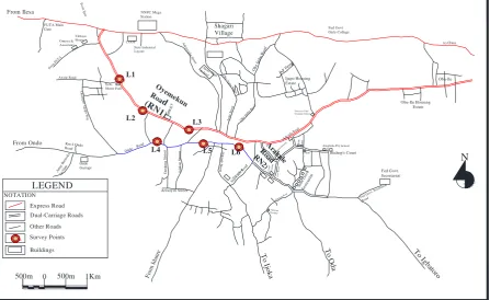
with BS 4142, 1997 using 407780A Integrating Sound Level Meter which conform with international electrotechnical commission (IEC) 61672. Measurements of traffic noise, spot speed and traffic volume variables were performed during the peak period (8:00am -9:00 am & 4:00pm-5:00pm) and off peak period (12:00-1:00pm). The measurement was repeated 3-5 times to account for time-fluctuation of these variables, while keeping in view the traffic and population densities. The noise levels were recorded in decibel (dB), while spot speeds and traffic volume count were recorded for all categories of vehicles using cine camera at six locations viz Ilesha Garage (L1), Adegbola (L2), Oba Market (L3), Isikan (L4), Post-office Junction (L5) and Eco Bank Junction (L6), the cine-camera was replayed to extract the data. Measurements were carried out every 15 s for a period of 15 min/h, this was considered to represent the variations in noise levels of the entire hour. Table 2 is the percentage evaluation of passenger’s car unit, while Figure 1 is the road network map of Akure showing the selected sites.

3. 3. 3.

3. RESULTRESULTRESULTRESULTSSSS AND DISCUSSIONAND DISCUSSIONAND DISCUSSIONSSSSAND DISCUSSION

3.1 3.1 3.1

3.1 Calculation of Equivalent Noise Level (LAeq)Calculation of Equivalent Noise Level (LAeq)Calculation of Equivalent Noise Level (LAeq)Calculation of Equivalent Noise Level (LAeq) The equivalent noise levels (LAeq) at the selected locations were evaluated using equations (1), (3) and (4) respectively. Using Burgess model in equation (1), KLMN O 78.24 \|(L), Using British Standard-5228 Model in equation (3), and noting that KngO 10logij}~_~•_€•

‚

(4)

pressure and P0 is magnitude of reference pressureO

20mPa

KgTUO 74.61 \|(L)

Using FHWA Model in equation (4), we get: KLTUO 78.05 dB(A) dB(A)

Similarly, the average equivalent noise level during the peak and off-peak period were calculated in the same manner for other locations using three models, the summary is shown in Table 3. Also, Figure 2 and Figure 3 are the graph of the observed Sound Exposure Level versus the predicted Sound Exposure Level (LAeq) for the selected road network.

4444.... CONCLUSIONCONCLUSIONCONCLUSIONCONCLUSION

The average equivalent noise level on the road network in the study area using Burgess model, British standard model and FWHA model are 77.64 dB(A), 72.95 dB(A)and 75 dB(A) respectively. The values

obtained using Burgess and FWHA model were higher than 75 dB(A) recommended by Policy on Traffic Noise Abatement 2011; while that obtained using British standard model is lower. However, the noise levels predicted by Burgess model and FWHA model also lies within an error band of ± 5% with reference to the observed noise levels. Thus, the three models are effective in predicting equivalent traffic noise index in Akure within a fair degree of accuracy. Also, 0.931 and 0.968 were obtained as the coefficient of correlation (R2_{) for Oyemekun road (RN1) and}

Arakale road (RN2) when observed Sound Exposure Level was plotted against the predicted Sound Exposure Level (LAeq); thus, there is a good correlation between the observed and the predicted value. Road traffic noise can be reduced through adequate road design, management of traffic flow and the use of screens and barriers.

Table 3: Summary of Average Equivalent Noise Level

Road Location Period T Ui Q H L SEL

Burgess Model Leq(1hr)

British Standard Leq(1hr)

FHWA Leq(1hr) (sec) (km/hr) (veh/min) (%) (%) dB(A) dB(A) dB(A) dB(A)

OY

EM

EK

UN

(R

N1

) _L1 Peak 1.55 23.55 33.33 1.10 98.76 76.77 78.65 74.61 78.05

Off-Peak 1.52 32.95 30.36 1.31 98.69 77.23 78.24 72.81 78.33

L2 Peak 1.44 24.96 35.38 1.15 98.79 76.00 78.91 74.53 77.35 Off-Peak 1.31 27.90 33.97 0.85 99.04 74.67 78.73 73.72 75.47

L3 Peak 1.29 29.31 29.93 2.44 97.57 75.52 78.19 73.07 75.97 Off-Peak 1.13 31.98 31.49 2.92 97.08 74.80 77.62 72.05 74.53

AR

AK

AL

E

(R

N2

) L4 Peak 1.55 23.51 23.81 1.78 98.22 77.70 77.16 73.21 79.12 Off-Peak 1.53 23.60 21.82 1.38 98.62 74.70 76.77 72.45 74.83

L5 Peak 1.33 27.22 24.51 1.56 98.44 77.08 77.29 72.67 78.42 Off-Peak 1.25 28.73 22.33 1.66 98.34 76.50 76.88 72.23 77.27

L6 Peak 1.33 27.17 21.21 2.45 97.55 77.47 76.65 72.10 78.30 Off-Peak 1.37 26.22 20.99 2.32 97.68 75.70 76.60 71.94 75.93 Noise Level for Commercial area dB(A) 77.64 72.95 75.00

Figure 2: Observed Sound Exposure Level versus the Predicted Sound for RN1 y = 1.442x - 32.73

R² = 0.931

73.0 74.0 75.0 76.0 77.0 78.0 79.0 80.0 81.0

73.0 74.0 75.0 76.0 77.0 78.0 79.0

O

B

S

E

R

V

E

D

S

O

U

N

D

P

R

E

S

U

R

E

CALCULATED NOISE LEVEL

LAeq(T)

(5)

Nigerian Journal of Technology,

Nigerian Journal of Technology, Vol. 33, No. 4, October 2014Vol. 33, No. 4, October 2014 Figure 3: Observed Sound Exposure Level versus the Predicted Sound for RN2

REFERENCE REFERENCE REFERENCE REFERENCESSSS

E1] Abbaspour, M., Golmohammadi, R., Nassiri, P., Mahjub, H., (2006). An Investigation on Time-Interval Optimization of Traffic Noise Measurement. Journal of Low Frequency Noise Vibration & Active Control, Vol. 25 No. 4: 267-273.

E2] Acoustic Society of Japan (ASJ) Model (1998): Road Traffic Noise Prediction Model; Transportation Research Board Part 1

E3] Adie D.B., Otun J.A,Okuofu C.A. and Nasiru A. (2012): Assessment Of Noise Generated By Operations Within The Gunduwawa Quarry In Kano State, Nigeria; Nigerian Journal of Technology Vol. 31, No. 3, pp. 314-320.

E4] W, Ising H, Gallacher J. E. J, Sweetnam P. M. and Elwood P. C. (1999):Traffic Noise and Cardiovascular Risk: The Caerphilly and Speedwell Studies, Third Phase-10-Year Follow Up; Archives of Environmental Health, Taylor & Francis Vol. 54, No. 3, pp 210-216, E5] BS 5228-1(2009): Code of Practice for Noise and

Vibration Control on Construction and Open Sites– Part 1:

E6] Burgess, M. A. (1977): Noise Prediction for Urban Traffic Conditions-Related to Measurements in the Sydney Metropolitan Area. Applied Acoustics, Vol. 10: 1-7.DOI: 10.1016/0003-682X (77)90002.

E7] Graham J. M. A, Janssen S. A, Vos H, and Miedema H. M. E (2009): Habitual Traffic Noise at Home Reduces Cardiac Parasympathetic Tone during Sleep. International Journal of Psychophysiology Vol. 72 No.2, pp. 179-186.

E8] Ljungberg JK and Neely G (2007): Stress, Subjective Experience and Cognitive Performance during Exposure to Noise and Vibration. Journal of Environmental Psychology Vol. 27 No.1, pp. 44-54. E9] Mansouri, N.A., Pour Mahabadian, M., Ghasemkhani,

M (2006). Road Traffic Noise in Downtown Area of Tehran, Iranian Journal of Environmental Health Science and Engineering, Vol. 3 No.4: 261-266. E10] Ohrstrom E and Rylander R (1990). Sleep

Disturbance by Road Traffic Noise-A Laboratory Study on Number of Noise Events; Journal of Sound and Vibration Vol. 143 No. 1, pp. 93-101.

E11] Ondo State Ministry of Land and Housing, 2010: Road Network Map of Akure

E12] Oyedepo O.J. Ekom R.I. and Ajala K.A (2013): Analysis of Traffic Noise along Oyemekun-Oba Adesida Road Akure Ondo State Nigeria; Journal of Engineering Science and Technology Review Greece Vol. 6 No.1, pp 72-77.

E13] Ross, M., Brain & Wolde, T., (2001): Noise from Traffic as A Worldwide Policy Problem; Noise Control Engineering Journal, Vol. No.49 No.4, pp 159-161. E14] Rylander R (2004): Physiological Aspects of Noise-

Induced Stress and Annoyance. Journal of Sound and Vibration Vol. 277 No.3, pp. 471-478.

E15] Stefano, R. Danato, D. and Morri, B. (2001): A Statistical Model for Predicting Road Traffic Noise on Poisson Type Traffic Flow; Noise Control Engineering Journal, Vol.49 No. 3: 137-143.

E16] World Health Organization, (2005): United Nations Road Safety Collaboration: A Handbook of Partner Profiles, Geneva.

y = 1.345x - 25.59 R² = 0.968

70.0 72.0 74.0 76.0 78.0 80.0 82.0 84.0 86.0

72 74 76 78 80 82

O

B

S

E

R

V

E

D

S

O

U

N

D

P

R

E

S

U

R

E

CALCULATED NOISE LEVEL

LAeq(T)