Saturated water conductivity estimation based on X-ray CT images
– evaluation of the impact of thresholding errors
Bartłomiej Gackiewicz *, Krzysztof Lamorski , and Cezary Sławiński Institute of Agrophysics, Polish Academy of Sciences, Doświadczalna 4, 20-290 Lublin, Poland
Received May 22, 2018; accepted August 7, 2018
*Corresponding author e-mail: [email protected] © 2019 Institute of Agrophysics, Polish Academy of Sciences A b s t r a c t. X-ray computed tomography soil studies rely on
image analysis procedures that commonly begin with a thres-holding step which is prone to errors and leads to uncertainty in the deduced values of soil characteristics, e.g., total porosity, specific surface or simulated saturated water conductivity. In this paper, four 3D images of soil cores were thresholded using two different algorithms. Total porosity and specific surface were determined for binarized images whereas saturated water con-ductivity was numerically estimated using the Navier-Stokes equation-based modelling. The study shows that an errone-ous thresholding step leads to uncertainty in the determination of soil pore system characteristics and saturated water conduc-tivity estimation. The lowest relative error in the total porosity determination, which was obtained in our study, was 15%, and the highest 40%. The results of this study demonstrate that errors related to thresholding may have a huge impact on the estima -tion of saturated hydraulic conductivity in soils, easily reaching a relative error of 50% of the saturated water conductivity refe-rence value. Even small shifts in the threshold level can cause huge changes in saturated water conductivity estimation (a thres-hold shift by 6.7% for sample 2 analysed in the study caused more than a two-fold increase in the estimated value of saturated hydraulic conductivity).
K e y w o r d s: X-ray CT, soil porosity, thresholding, water conductivity
INTRODUCTION
X-ray computed tomography (CT) isa non-destructive imaging technique which can be used to study soil
proper-ties related to soil structure, i.e. soil pore space imaging. CT may also be used for imaging the whole soil core samples where a voxel size between 20 µm and 50 µm is achieved (Jarvis et al., 2017; Rab et al., 2014; Vaz et al., 2011). A resolution of this order allows for macropore observation (Jarvis, 2007; Katuwal et al., 2018; Müller et al., 2018) and root visualization (Daly et al., 2018; Sander et al., 2008). However, it can also be used for imaging soil aggregates
with a voxel size of 1 µm or smaller (Józefaciuk et al., 2015; Voltolini et al., 2017b). A 3D image obtained with this technique, following its processing, allows researchers to examine the inner structure of soil, and to collect infor-mation about pore distribution (Hu et al., 2015) and pore properties, such as shape factors (Elliot et al., 2010), con-nectivity (Sleutel et al., 2008) or pore circularity (Yang et al., 2018). The link between soil cores macroporosity and saturated water conductivity has been of special interest (Gerke, 2012; Larsbo et al., 2016; Müller et al., 2018).
In addition to the abovementioned soil characterization options which utilize CT, it is possible to model transport properties in porous materials using spatial models based on CT 3D images. CT-based modelling is an established approach with various applications, including fluid trans-port (Bultreys et al., 2016; Jiang et al., 2017; Starnoni et al., 2017), fluid-microstructure interaction (Lesueur et al., 2017), petrophysical transport (Liu et al., 2015), immisci-ble two-phase flow (Liu and Wu, 2016), reactive transport (Menke et al., 2017) or carbonate dissolution (Pereira Nunes et al., 2016). The use of real soil structures for building models allows researchers to better understand the pore-scale processes (Daly et al., 2017, 2018; Wildenschild and Sheppard, 2013; Zhang et al., 2016).
However, both the CT-based modelling and the soil characterization methods based on 3D image analyses may be inaccurate. A crucial step in the analysis of CT soil images involves segmentation which is used to divide a 3D image into solid particles and pore-space. Uncertainty relat-ed to threshold level determination is a common problem in the image analysis practice (Baveye et al., 2010; Iassonov
et al., 2009). This is especially common when the
one might expect vast differences in the obtained results, and possibly a high impact on the results of modelling based on pore-space geometry. The choice of the segmen-tation method has a significant impact on the calculation of soil parameters, such as porosity (Baveye et al., 2010). The proper segmentation of a 3D image into solid and pore-space is important to create the right 3D pore-pore-space model. The segmentation step may also be influenced by the image filtering process preceding binarisation (Smet et al., 2018).
There is no standard procedure for image segmenta-tion because of the diversity of porous materials. A 3D CT image consists of voxels of different gray values, reflect-ing the X-ray absorption in a given space. Therefore, CT image segmentation can be performed by setting the thresh-old value below or above which voxels will be allocated to one or another set, respectively. Global thresholding, which uses the same threshold value for binarizing the whole image, can be performed manually (Baveye et al., 2010; Moreira et al., 2012) or automatically (Andrä et al., 2013;
Daly et al., 2017; Iassonov et al., 2009; Sezgin and Sankur, 2004; Schläuter et al., 2014). A semi-automated approach can also be used (Latief et al., 2017).
However, a CT image is not an ideal representation of X-ray absorption in a given matter. The space in a 3D digital image is discretised, phase boundaries do not usu-ally coincide with boundaries of voxels, and dimensions of some particles can be below the CT resolution (Jones and Feng, 2016). Additionally, other scanning artifacts, such as noise, beam hardening or scattered X-rays (Helliwell et al., 2013; Houston et al., 2013; Wildenschild et al., 2002), can reduce the accuracy of global thresholding.
Another approach involves locally-adaptive segmen-tation methods (Hapca et al., 2013; Katuwal et al., 2018; Martín-Sotoca et al., 2018; Porter and Wildenschild, 2010). Some of these have been designed especially for binarising the soil media (Hapca et al., 2013; Martín-Sotoca et al.,
2018) which utilize spatial information beside the gray le-vel value to assign each voxel to a pore-space or soil matrix. Yet another approach uses both the global thresholding and the locally-adaptive methods (Voltolini et al., 2017a). Although local segmentation methods are known to be gen-erally more accurate, they may be more sensitive to various imperfections of a CT reconstructed image. Furthermore,
local thresholding methods are much more computationally
demanding. For these reasons, global thresholding algo-rithms are still frequently used in practice.
The global thresholding methods considered to be suita-ble for soil images (Hapca et al., 2013) include Otsu (1979) and Ridler’s techniques (Ridler and Calvard, 1978). The Ridler’s method, being an iterative self-organizing data analysis technique, is a simple thresholding method which finds application in the study of soil images (Rab et al., 2014; Wang et al., 2011) and images of other porous mate-rials (Chen et al., 2018; Liu et al., 2013; Than et al., 2017).
To ensure the correctness of CT-based soil charac-terizations, it should be checked whether the 3D model correctly reproduces the actual pore network of the sample. Validation can be performed by comparing the param-eters estimated on the basis of a 3D image with those measured in the laboratory. Some of them, like porosity, can be obtained directly from a CT image analysis (Smal
et al., 2018) whereas other demand a modelling process. Hydraulic conductivity is a parameter that can be easily obtained through laboratory measurements and estimated in a computer simulation. There are three main approaches to pore-scale modelling, i.e. the lattice Boltzmann method (Gao et al., 2015; McClure et al., 2014), the pore network modelling (Bultreys et al., 2015; Ngom et al., 2011) and the Navier-Stokes (NS) model (Icardi et al., 2014; Muljadi et al., 2016). NS models are differential equations which can be discretised in different manners, e.g. by means of the finite volume method (FVM), the finite difference method (FDM) or the finite element method (FEM). The FVM is popular for its computational efficiency (Bultreys et al., 2016; Meakin and Tartakovsky, 2009) and for the use of unstructured meshes that can be applied easily to complex pore space geometry.
The thresholding step, which usually begins with image
analysis procedures, seems to have a crucial impact on the
obtained results. This is especially true for the analysis of soil which is a heterogeneous medium that is prone to errors caused by improperly made image binarisation. The impact
of the thresholding method on porosity determination for
soil media has already been extensively investigated, e.g., by Baveye et al. (2010). Also the impact of thresholding on modelling of the soil water retention curve (SWRC) and deduced from the SWRC unsturated water conductivity was investigated by Beckers et al. (2014). Although seve-ral works exist which discuss the possible impact of the
segmentation step on different soil media properties, the
authors, using their best knowledge, have not come across any analysis related to the possible impact on the modelling of saturated water conductivity. The aim of our work was to evaluate the impact of the possible thresholding inaccuracy on saturated water conductivity estimations. The uncer-tainty in determining other soil pore-space characteristics, such as total porosity and image specific surface, was also investigated.
MATERIALS AND METHODS
For the purpose of this study, four soil cores were tested, and two soil types (described inTable 1) differing in micro-structure were chosen. Samples 1 and 2 are mineral (Orthic Luvisol) soil while samples 3 and 4 are organic peat soil (Eutric Histosol). Cores were sampled from two different locations by taking two samples from each location. The samples were taken from arable layers, five centimetres below the soil surface. Sampling took place in the spring 2017 when soil moisture was high enough to use plastic cylinders for sampling. Soil moisture also allowed for the sampling to be performed without the risk of soil structure destruction. Plastic cylinders were 45 mm in diameter and 40 mm in height, and they were not as strong and stiff as metal ones but had a lower X-ray absorbance. The collected samples remained in cylinders for CT scans, in order not to change the structure of the sampled soil. Just after their col-lection, the samples were sealed with Parafilm to prevent water loss due to evaporation, which could lead to
shrink-ing of the soil sample and, consequently, to changes in its
structure.
The samples placed in plastic cylinders were exam-ined using an X-ray computational micro-tomograph GE Nanotom 180S at the IA PAS X-ray CT facility (Lamorski, 2017). Parameters of the X-ray tube were as follows: the accelerating voltage 100 kV, the cathode current 150 μA, and a tungsten exit window. An exit window filter was not used. During the scan, a series of 1200 2D images were registered by rotating the sample by 0.3˚ stepwise for a full 360-degree rotation. For noise reduction purposes, each 2D image was averaged out of 20 records that were 750 ms
each, which were acquired with a slight (by a few pixels) random perpendicular angle to the X-ray beam detector movements. The 2D images were registered with a 14-bit gray level depth by a flat panel detector with a resolution of 2 284x2 304 pixels.
After the X-ray CT examination of the samples, satu-rated water conductivity of the cores was measured repeatedly, using the constant head method (Eijkelkamp Soil and Water, The Netherlands) (Table 1).
The 3D reconstruction, using the collected 2D images, was performed with CT software (datos|x version 2.0.1, General Electric). It was necessary to use the software beam hardening correction offered by CT reconstruction software. The spatial resolution of the 3D reconstructed
volume, i.e. voxel size, was 23.6 µm in each direction. The 3D images were saved as 16-bit tiff files. The selection of the cylindrical region of interest (ROI) for further process-ing, based on the reconstructed 3D volume, as well as the filtering process were performed using Avizo 9 (Thermo Fisher Scientific). The ROI had a cylindrical shape with a diameter 1 878 pixels. The ROI height were slightly dif-ferent for difdif-ferent samples and are presented in Table 1. The image was filtered twice for noise reduction, using a 3D median filter with a cross-shaped 3D kernel, with a dia-meter equal to 3 pixels. After the thresholding, pore size distribution was performed, which consisted of two steps, i.e. pore-space splitting and labelling. After the labelling, the dataset was generated with individual pore volumes and pore equivalent diameters.
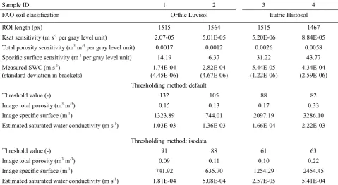
Table 1. Soil samples basic information: sample ID, FAO soil classification, measured saturated water conductivity and parameters obtained from analysis of CT imaging of samples
Sample ID 1 2 3 4
FAO soil classification Orthic Luvisol Eutric Histosol
ROI length (px) 1515 1564 1515 1467
Ksat sensitivity (m s-1 per gray level unit) 2.07-05 5.01E-05 5.20E-06 8.84E-05
Total porosity sensitivity (m3 m-3 per gray level unit) 0.0017 0.0012 0.0026 0.0058
Specific surface sensitivity (m-1 per gray level unit) 14.19 6.37 31.22 43.77
Measured SWC (m s-1)
(standard deviation in brackets) (4.45E-06)1.74E-04 (4.67E-06)2.82E-04 (1.22E-06)5.44E-05 (2.59E-06)4.34E-04 Thresholding method: default
Threshold value (-) 132 105 88 82
Image total porosity (m3 m-3) 0.15 0.13 0.17 0.33
Image specific surface (m-1) 1323.89 744.01 2097.19 3286.10
Estimated saturated water conductivity (m s-1) 1.03E-03 1.36E-03 1.66E-04 2.22E-03
Thresholding method: isodata
Threshold value (-) 91 88 61 63
Image total porosity (m3 m-3) 0.09 0.11 0.10 0.22
Image specific surface (m-1) 741.92 635.70 1254.29 2454.45
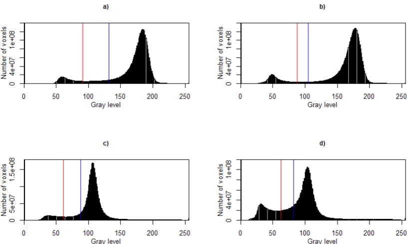
The filtered 16-bit 3D images of soils were converted into an 8-bit grayscale. The histograms (for the whole 3D image) of the scanned samples are shown in Fig. 1. Three of them are clearly bimodal (i.e. one can observe two maxima in the histogram) although the peak corresponding to the
solid is much larger than the one corresponding to the pore
space. Then, the 3D images were thresholded to distinguish pore-space from the soil solid phase, within the accuracy level for which the µCT scan resolution was achieved. Two different threshold methods were applied in respect of all the 3D images. The thresholding was performed using the Fiji image processing software (Schindelin et al., 2012). Two global thresholding algorithms available in Fiji, i.e.
‘Default’ and ‘Isodata’, were used to this end. Both meth-ods are variations of Ridler’s iterative intermeans algorithm (Ridler and Calvard, 1978). The difference between both algorithms is that the ‘Default’ method uses some additional histogram pre-processing prior to applying the intermeans
algorithm. The pre-processing modifies the maximum peak in the cases where it is more than twice higher in relation to the other. The images that were thresholded by the Default and Isodata methods will be hereinafter referred to as ‘the Default threshold’ and ‘the Isodata threshold’, respectively.
The process of thresholding consisted of two stages. Firstly, a single slice (an example of the slice is shown in Fig.2) was arbitrarily chosen as the most representative (with no artifacts, clearly observed pores and a structure similar to other slices) for the whole 3D volume, based on which a histogram of gray values was calculated. The obtained gray level threshold value was used rather than binarizing the whole 3D volume. This approach was based
on the selection of a representative slice for threshold calcu
-lation, instead of determining separate thresholds for each
slice in the stack to avoid incorrect thresholding results for the slices without proper pore representation (Iassonov
et al., 2009).
Fig. 1. Histograms of the scanned soil cores: a) - sample 1, b) - sample 2, c) - sample 3, d) - sample 4 with marked values of the isodata threshold (red line) and the default threshold (blue line).
In this study, two different algorithms of thresholding were evaluated. The reasons for choosing these algorithms were of a twofold nature. Firstly, they are commonly used for porous media studies including soils (Hapca et al., 2013) and, secondly, the evaluation of different algorithms based on the thresholding of selected slices from soil cores shows more optimal results in comparison with other approaches. There is one specific aspect of the algorithms in question which qualifies them for application to the soil core seg-mentation task, i.e. they do not rely on the assumption
of the bimodal character of the histograms of segmented images as does, for example, the popular Otsu method. It is uncommon to see true bimodal histograms in X-ray CT soil related studies, due to the fact that CT-detected pores only
form a small fraction of the scanned core volume ≲0.2. The Otsu method has also been used in soil related CT studies,
e.g., in the work by Jarvis et al. (2017).
The threshold values are presented in Table 1 in a 256-degree scale, where 0 corresponds to the black voxels and 255 represents white voxels.
In the thresholded binary image, there are two types of voxels representing pore-space and soil solid phases. Such a voxelized surface of the pore-space would not be a good representation of the physical surface. It was interpolated using the triangulation method with a BoneJ plugin (Doube
et al., 2010) and then saved as a STL file for further use in numerical mesh generation. The image total porosity and the image specific surface were also determined (Table 1). The image specific surface σ (m-1) was calculated as the
area of a triangulated surface (m2) divided by the ROI
volume (m3).
For transport modelling, NS equations were used. The set of NS equations comprises the momentum balance Eq. (1) and the continuity Eq. (2), where u is a velocity vector
(m s-1), ρ is fluid density (kg m-3), p is pressure (kg m-1 s-2),
µ is dynamic viscosity (kg m-1 s-1), τ is a strain rate ten
-sor (s-1), F are external forces (kg m s-2) (Eq. (3)), and g is
gravitational acceleration (m s -2):
(1)
(2)
F = p g. (3)
It was implemented by means of the OpenFOAM CFD software, using FVM differential equation discretisation. For the simulation purpose, a non-compressible steady-state laminar single phase flow was assumed. The flow domain was the CT-determined sample macropore network while the remaining part of the sample was treated as a non-permeable solid body.
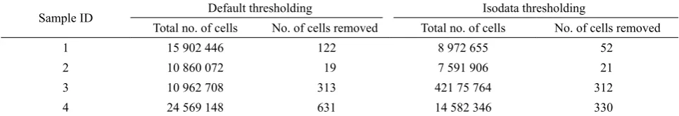
OpenFOAM uses unconstrained and unstructured meshes which are especially suitable for the meshing of complex pore-space geometry. The numerical mesh was created on the basis of the STL file with a triangulated surface of the soil solid phase, using snappyHexMesh – a native OpenFOAM meshing tool which allows for the meshing of non-uniform complex geometries. Mesh cells were generated only for the pore-space regions of soil, and for additional thin layers connected with pores at both the input and output on which boundary conditions were enforced. However, OpenFOAM software focuses on gen-erating high quality mesh, although in such a complex meshed geometry as in the case of pore-space some of the mesh cells do not always meet quality constraints. To avoid such potential problems, the created mesh was checked for the occurrence of cells with highly skewed faces. Faces with the skewness value being higher than four were delet-ed. The presence of cells with highly skewed faces could impair the quality of the results and make the calculations unstable. The number of deleted cells is shown in Table 2. As it did not exceed 0.003% of the total number of cells, it can be assumed that the impact of deleted cells on the geometry of the whole image was negligible.
The numerical mesh simulations were performed using a steady-state simpleFoam solver. The appropriate bound-ary conditions were set up in the simulation process, i.e. the
value of fluid velocity was fixed to 1e-5 m s-1, and the pres
-sure was established at 0Pa on the input patch with zero gradient Neuman conditions on the output patch. The input and output patches were equivalent to the top and bottom portions of the soil sample. No-slip boundary conditions were applied to the pore walls.
The water flow simulation mimics the constant head saturated conductivity measurement principle. Saturated
hydraulic conductivity Ks (m s-1) can be estimated based
Table 2. Statistic of numerical mesh used for SWC modeling (total No. of cells – total number of cells in the mesh, No. of cells removed – number of cell removed from mesh due to quality constraints)
Sample ID Default thresholding Isodata thresholding
Total no. of cells No. of cells removed Total no. of cells No. of cells removed
1 15 902 446 122 8 972 655 52
2 10 860 072 19 7 591 906 21
3 10 962 708 313 421 75 764 312
on information about pressure difference Δp (kg m-1 s-2)
between the input and output patches, fluid velocity at the
input patch u (m s-1) and flow domain length Δl (m):
, (4)
where: g (m s-2) stands for gravitational constant and ρ
(kg m-3) for fluid density.
A sensitivity analysis allows for estimating the impact of the perturbation in the model’s input parameters on the model’s output. The local sensitivity analysis is used for
sensitivity estimation for a given value or a set of selected
values of input parameters. On the other hand, the global sensitivity analysis allows for the general quantification of sensitivity for the whole range of input parameters.
More general approaches are available for sensiti-vity estimation, including the one-factor-at-a-time method (OAT), the Morris method or variance decomposition based methods (Saltelli et al., 2002). In the simplest cases where local sensitivity estimation is needed and models input parameters are not correlated, a differential sensiti-vity analysis can be performed (Hamby, 1994) instead.
The differential sensitivity analysis is based on the assumption that sensitivity coefficient Si for a particular
independent variable Xi may be estimated by the partial
derivative of dependent variable Y (i.e. the model’s output) with respect to an independent variable (i.e. the model’s
parameter):
(5)
Obviously, in practical applications partial derivatives have to be estimated by finite differences because the mo-dels are not usually described by analytical functions which could be differentiated.
RESULTS AND DISCUSSION
The intermeans algorithm based thresholding proce-dures, which was used in this study, unlike the popular Otsu method, does not rely on the histogram bimodality assump-tion. In the soil samples studied, the problem of histogram non-bimodality can also be observed, as evidenced in the histograms for samples 2 and 4 (Fig. 1b, d). These samples are bimodal, although the maximum values related to pores are much lower than the maximum values related to the soil matrix. However, it is hard to treat the histograms of samples 1 and 3 as bimodal, especially since the histogram of sample 3 completely lacks this feature (Fig. 1a, c).
Two different variations of the iterative intermeans algorithm were evaluated in this study, i.e. Default and
Isodata. For the examined samples, the threshold values were always higher in the case of the Default thresholding algorithm. The higher value of the threshold is connected with a higher number of voxels categorized as correspond-ing to the pore space and, hence, with higher porosity. As
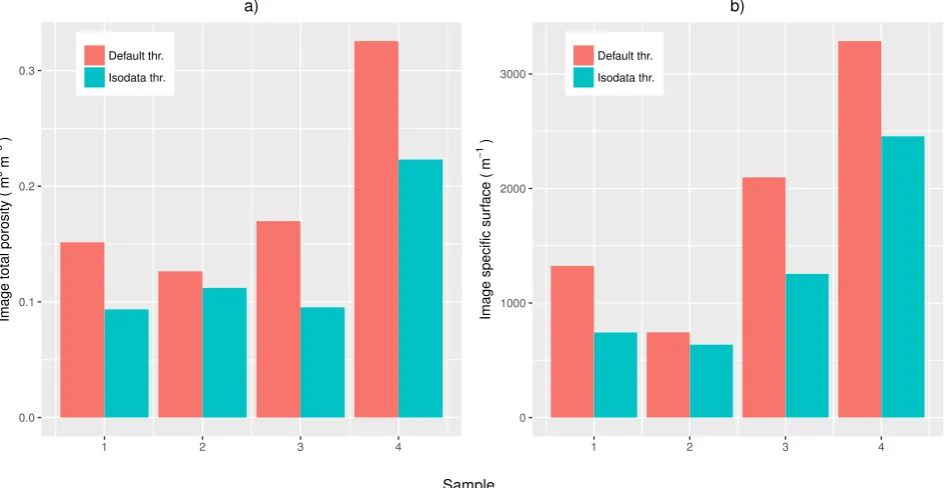
can be observed in Fig. 1, different values of thresholds are determined using different validated algorithms. The Isodata threshold algorithm always places a lower value of the threshold which means that the smaller part of the sam-ple’s volume is considered to be a pore-space. Differences in the threshold levels determined by these two algorithms ranged from 17 to 41 units, where 8-bit depth and 256 gray levels were used for CT image representation. Similar va-lues of the threshold levels achieved by different algorithms were reported (Smet et al., 2018) for soil media. A sample slice from the stack representing sample 1 is presented in Fig.2. It can be seen that the default thresholding algo-rithm area of the pores on this cross-section is bigger than in the case of the Isodata algorithm. The differences in total porosity that were detected using CT for the presented sam-ples were as follows: 0.06, 0.02, 0.07 and 0.11, respectively (Fig. 3). It means that the minimum change in porosity was 15%, and the maximum change was 40%, in rela-tion to the porosities determined by means of the Default algorithm (Table 1). Both porosities, determined for the Default and Isodata thresholded media, are well-correlated, R2 = 0.9 (Fig. 4).
These results show that the potential impact of the im-proper selection of the thresholding method on porosi-ty results is high, and this phenomenon has already been identified in literature (Baveye et al., 2010). The sensitivity indices which were calculated and analyzed in the study confirm this point of view (Table 1). If we assumed the pos-sible uncertainty in the threshold level determination at ten units, corresponding to 4%, it would cause uncertainty in the total porosity determination of at least 10% for sample 1 (with 17% being the highest value calculated for sample 4).
So, an erroneous determination of the threshold value
propagates a porosity determination error and boosts it sub-stantially. It is worth mentioning that 10 uncertainty units used in the present discussion reflect a realistic assumption
as far as differences in the threshold level determination
are concerned (Wang et al., 2011). The differences in the threshold level determination in soil studies may be even higher (Beckers et al., 2014).
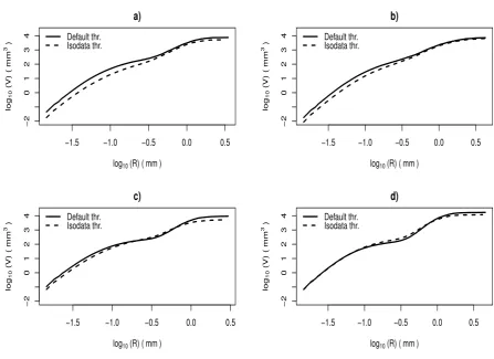
Threshold changes exert a varied impact on pores with different sizes, which is reflected in the cumulative pore distribution (Fig. 5). In the case of samples 1 and 2, pores with different volumes increase proportionally for the samples thresholded by means of the Default and Isodata algorithms. In the case of samples 3 and 4, the volume of pores with an equivalent radius up to ~0.1-0.2 mm increas-es proportionally whereas porincreas-es with higher radiusincreas-es, up to ~0.7 mm, dominate in the case of the Isodata thresh-olded samples. Finally, once the radius value of ~0.7 mm was achieved in both samples 3 and 4, thresholded by the
Default algorithm, an increase in the volume of largest
As in the case of total porosity, the image specific
sur-face is also dependent on the threshold methods applied in
the image analysis workflow (Fig. 3). The highest change in specific surface is observed for sample 1 – 80%, and smallest for sample 2 – 17%, in relation to the default thresholding method (Table 1). Both characteristics are well-correlated, R2 = 0.95 (Fig. 6). The sensitivity analysis
allows us to estimate the potential impact of the thresh-old level determination inaccuracy on the image specific
surface determination. Assuming the same threshold
deter-mination uncertainty, i.e. reaching ten units of inaccuracy,
the specific surface determination would be at least 64 (m-1)
and maximum inaccuracy would be 437 (m-1).
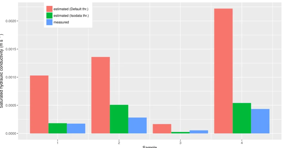
Two simulations based on different thresholding meth-ods were made, and different values of saturated hydraulic conductivity estimations were obtained (Fig. 7). Values of the SWC estimated with the NS model on the basis of the de-fault threshold are well correlated with the corresponding
Fig. 3. Values of the image total porosity (a) and the image specific surface (b) determined on the basis of 3D soil images thresholded with the Isodata method (red) and the Default (green) method.
Fig. 5. Cumulative pore volume distributions for pore spaces (R-equivalent pore radius) determined using the Default algorithm (con-tinuous line) and the Isodata algorithm (dashed line). a – sample 1, b – sample 2, c – sample 3, d – sample 4.
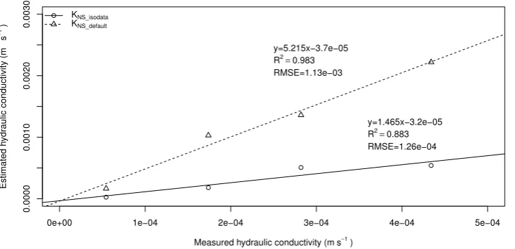
values estimated by means of the Isodata threshold, R2 = 0.83. The Isodata-based estimations are, on average,
three times lower than the Default thresholding-based esti-mations (Fig. 8). Both estiesti-mations are highly correlated with the measured values of SWC (R2=0.98 for Default
thresholding and R2 = 0.88 for Isodata thresholding), but
the Default threshold-based simulations overestimate five times saturated water conductivity (Fig. 9), when compared with the measured values. The Isodata threshold-based simulations are much accurate, with only a slight ~1.5 overestimation.
The local sensitivity indices calculated for SWC (Table 1) show a strong dependence of the SWC on the
potential uncertainty related to threshold level determi -nation. The lowest Ksat sensitivity coefficient value is ~5.2e-6, and the highest ~8.8e-5 (m s-1 per gray level unit]. If the previous assumption of the uncertainty related to
threshold level determination was adopted at 10 gray level units, it would lead to the uncertainty in SWC estimation ranging from 5.2e-5 to 8.8e-4 (m s-1), based on the results
of our study. If these errors were compared to the SWC estimations based on the Default threshold, they would cor-respond to relative error values of 20 and 40%, respectively.
Fig. 7. Saturated water conductivity: estimations based on differently-thresholded images and laboratory measurements.
Wei Q., and Sezgin M., 2010. Observer-dependent varia-bility of the thresholding step in the quantitative analysis of soil images and X-ray microtomography data. Geoderma, 157, 51–63. doi:10.1016/J.GEODERMA.2010.03.015 Beckers E., Plougonven E., Roisin C., Hapca S., Léonard A.,
and Degré A., 2014. X-ray microtomography: A porosity-based thresholding method to improve soil pore network characterization? Geoderma, 219-220, 145-154, doi:10. 1016/j.geoderma.2014.01.004
Bultreys T., De Boever W., and Cnudde V., 2016. Imaging and image-based fluid transport modeling at the pore scale in geological materials: A practical introduction to the current state-of-the-art. Earth-Science Rev., 155, 93-128. doi:10.1016/J.EARSCIREV.2016.02.001
Bultreys T., Van Hoorebeke L., and Cnudde V., 2015. Multi-scale, micro-computed tomography-based pore network models to simulate drainage in heterogeneous rocks. Adv. Water Resour., 78, 36-49. doi:10.1016/J.ADVWATRES. 2015.02.003
Chen X., Verma R., Espinoza D.N., and Prodanović M., 2018. Pore-scale determination of gas relative permeability in hydrate-bearing sediments using X-ray computed micro-tomography and lattice Boltzmann method. Water Resour. Res. 54, 600-608. doi:10.1002/2017WR021851
Daly K.R., Cooper L.J., Koebernick N., Evaristo J., Keyes S.D., van Veelen A., and Roose T., 2017. Modelling water dynamics in the rhizosphere. Rhizosphere, 4, 139-151. doi:10.1016/J.RHISPH.2017.10.004
Daly K.R., Tracy S.R., Crout N.M.J., Mairhofer S., Pridmore T.P., Mooney S.J., and Roose T., 2018. Quantification of root water uptake in soil using X-ray com-puted tomography and image-based modelling. Plant. Cell Environ., 41, 121-133. doi:10.1111/pce.12983
Doube M., Klosowski M.M., Arganda-Carreras I., Cordelières F.P., Dougherty R.P., Jackson J.S., Schmid B., Hutchinson J.R., and Shefelbine S.J., 2010. BoneJ: Free and extensible bone image analysis in Image J. Bone, 47, 1076-1079. doi:10.1016/j.bone.2010.08.023
CONCLUSIONS
1. The results of this study demonstrate that threshold-ing-related errors may have a huge impact on the estimation
of saturated hydraulic conductivity in soils, easily reaching
a relative error that accounts for 50% of the saturated water conductivity reference value.
2. Even small shifts in the threshold level can cause huge changes in saturated water conductivity estimations. For instance, a threshold shift of 6.7% for sample 2 caused more than a two-fold increase in the value of saturated hydraulic conductivity.
3. Soil images are hard to threshold automatically because their histograms do not display explicit bimodali-ty, which eventually leads to thresholding errors. This is caused by the relatively small pore-space fraction observed
in the computed tomography images of soils.
4. The sensitivity of computed tomography-based esti-mations of saturated water conductivity on thresholding shows that the values estimated through modelling should be validated.
Conflict of interest: The authors declare no conflict of interest.
REFERENCES
Andrä H., Combaret N., Dvorkin J., Glatt E., Han J., Kabel M., Keehm Y., Krzikalla F., Lee M., Madonna C., Marsh M., Mukerji T., Saenger E.H., Sain R., Saxena N., Ricker S., Wiegmann A., and Zhan X., 2013. Digital rock physics benchmarks-Part I: Imaging and segmentation. Comput. Geosci., 50, 25-32. doi:10.1016/j.cageo.2012.09.005 Baveye P.C., Laba M., Otten W., Bouckaert L., Dello Sterpaio
P., Goswami R.R., Grinev D., Houston A., Hu Y., Liu J., Mooney S., Pajor R., Sleutel S., Tarquis A., Wang W.,
Elliot T.R., Reynolds W.D., and Heck R.J., 2010. Use of exist-ing pore models and X-ray computed tomography to predict saturated soil hydraulic conductivity. Geoderma, 156, 133-142. doi:10.1016/j.geoderma.2010.02.010
Gao J., Xing H., Rudolph V., Li Q., and Golding S.D., 2015. Parallel lattice Boltzmann computing and applications in core sample feature evaluation. Transp. Porous Media, 107, 65-77. doi:10.1007/s11242-014-0425-1
Gerke H.H., 2012. Macroscopic representation of the interface between flow domains in structured soil. Vadose Zo. J., 11, 0. doi:10.2136/vzj2011.0125
Hamby D.M., 1994. A review of techniques for parameter sensi-tivity analysis of environmental models. Environ. Monit. Assess., 32, 135-154. doi:10.1007/BF00547132
Hapca S.M., Houston A.N., Otten W., and Baveye P.C., 2013. New local thresholding method for soil images by minimiz-ing grayscale intra-class variance. Vadose Zo. J., 12, 0. doi:10.2136/vzj2012.0172
Helliwell J.R., Sturrock C.J., Grayling K.M., Tracy S.R., Flavel R.J., Young I.M., Whalley W.R., and Mooney S.J., 2013. Applications of X-ray computed tomography for examining biophysical interactions and structural develop-ment in soil systems: a review. Eur. J. Soil Sci., 64, 279-297. doi:10.1111/ejss.12028
Houston A.N., Schmidt S., Tarquis A.M., Otten W., Baveye P.C., and Hapca S.M., 2013. Effect of scanning and image reconstruction settings in X-ray computed microtomogra-phy on quality and segmentation of 3D soil images. Geoderma, 207-208, 154-165. doi:10.1016/J.GEODERMA. 2013.05.017
Hu X., Li Z.-C., Li X.-Y., and Liu Y., 2015. Influence of shrub encroachment on CT-measured soil macropore characteris-tics in the Inner Mongolia grassland of northern China. Soil Till. Res., 150, 1–9. doi:10.1016/j.still.2014.12.019 Iassonov P., Gebrenegus T., and Tuller M., 2009. Segmentation
of X-ray computed tomography images of porous materi-als: A crucial step for characterization and quantitative analysis of pore structures. Water Resour. Res., 45. doi:10.1029/2009WR008087
Icardi M., Boccardo G., Marchisio D.L., Tosco T., and Sethi R., 2014. Pore-scale simulation of fluid flow and solute disper-sion in three-dimendisper-sional porous media. Phys. Rev., E 90, 013032. doi:10.1103/PhysRevE.90.013032
Jarvis N., Larsbo M., and Koestel J., 2017. Connectivity and percolation of structural pore networks in a cultivated silt loam soil quantified by X-ray tomography. Geoderma, 287, 71-79. doi:10.1016/j.geoderma.2016.06.026
Jarvis N.J., 2007. A review of non-equilibrium water flow and solute transport in soil macropores: principles, controlling factors and consequences for water quality. Eur. J. Soil Sci., 58, 523-546. doi:10.1111/j.1365-2389.2007.00915.x Jiang Z., van Dijke M.I.J., Geiger S., Ma J., Couples G.D., and
Li X., 2017. Pore network extraction for fractured porous media. Adv. Water Resour., 107, 280-289. doi:10.1016/j. advwatres.2017.06.025
Jones B.D., and Feng Y.T., 2016. Effect of image scaling and segmentation in digital rock characterisation. Comput. Part. Mech., 3, 201-213. doi:10.1007/s40571-015-0077-0 Józefaciuk G., Czachor H., Lamorski K., Hajnos M., Świeboda
R., and Franus W., 2015. Effect of humic acids, sesquiox-ides and silica on the pore system of silt aggregates
measured by water vapour desorption, mercury intrusion and microtomography. Eur. J. Soil Sci., 66, 992-1001. doi:10.1111/ejss.12299
Katuwal S., Hermansen C., Knadel M., Moldrup P., Greve M.H., and de Jonge L.W., 2018. Combining X-ray com-puted tomography and visible near-infrared spectroscopy for prediction of soil structural properties. Vadose Zo. J., 17, 0. doi:10.2136/vzj2016.06.0054
Lamorski K., 2017. X-ray computational tomography facility - Institute of Agrophysics PAS [WWW Document]. URL http://tomography.ipan.lublin.pl/ (accessed 4.19.18). Larsbo M., Koestel J., Kätterer T., and Jarvis N., 2016.
Prefe-rential transport in macropores is reduced by soil organic carbon. Vadose Zo. J. 15, 0. doi:10.2136/vzj2016.03.0021 Latief F.D.E., Fauzi U., Irayani Z., and Dougherty G., 2017.
The effect of X-ray micro computed tomography image resolution on flow properties of porous rocks. J. Microsc., 266, 69-88. doi:10.1111/jmi.12521
Lesueur M., Casadiego M.C., Veveakis M., and Poulet T., 2017. Modelling fluid-microstructure interaction on elasto-visco-plastic digital rocks. Geomech. Energy Environ., 12, 1-13. doi:10.1016/J.GETE.2017.08.001
Liu J., Song R., and Cui M., 2015. Improvement of predictions of petrophysical transport behavior using three-dimension-al finite volume element model with micro-CT images. J. Hydrodyn., Ser. B, 27, 234-241. doi:10.1016/S1001-6058(15)60477-2
Liu Y., Wang H., Shen Z., and Song Y., 2013. Estimation of CO2
storage capacity in porous media by using X-ray micro-CT. Energy Procedia, 37, 5201-5208. doi:10.1016/J.EGYPRO. 2013.06.436
Liu Z., and Wu H., 2016. Pore-scale modeling of immiscible two-phase flow in complex porous media. Appl. Therm. Eng., 93, 1394-1402. doi:10.1016/j.applthermaleng.2015. 08.099
Martín-Sotoca J.J., Saa-Requejo A., Grau J.B., and Tarquis A.M., 2018. Local 3D segmentation of soil pore space based on fractal properties using singularity maps. Geoderma, 311, 175-188. doi:10.1016/J.GEODERMA.2016.11.029 McClure J.E., Prins J.F., and Miller C.T., 2014. A novel hetero
-geneous algorithm to simulate multiphase flow in porous media on multicore CPU-GPU systems. Comput. Phys. Commun., 185, 1865-1874. doi:10.1016/J.CPC.2014.03.012 Meakin P., and Tartakovsky A.M., 2009. Modeling and simula-tion of pore-scale multiphase fluid flow and reactive transport in fractured and porous media. Rev. Geophys., 47, RG3002. doi:10.1029/2008RG000263
Menke H.P., Bijeljic B., and Blunt M.J., 2017. Dynamic reser -voir-condition microtomography of reactive transport in complex carbonates: Effect of initial pore structure and ini-tial brine pH. Geochim. Cosmochim. Acta, 204, 267-285. doi:10.1016/j.gca.2017.01.053
Moreira A.C., Appoloni C.R., Mantovani I.F., Fernandes J.S., Marques L.C., Nagata R., and Fernandes C.P., 2012. Effects of manual threshold setting on image analysis results of a sandstone sample structural characterization by X-ray microtomography. Appl. Radiat. Isot., 70, 937-941. doi:10.1016/J.APRADISO.2012.03.001
flow behaviour from pore-scale simulation. Adv. Water Resour., 95, 329-340. doi:10.1016/J.ADVWATRES.2015. 05.019
Müller K., Katuwal S., Young I., McLeod M., Moldrup P., de Jonge L.W., and Clothier B., 2018. Characterising and linking X-ray CT derived macroporosity parameters to infiltration in soils with contrasting structures. Geoderma, 313, 82-91. doi:10.1016/j.geoderma.2017.10.020
Ngom N.F., Garnier P., Monga O., and Peth S., 2011. Extraction of three-dimensional soil pore space from microtomogra-phy images using a geometrical approach. Geoderma, 163, 127-134. doi:10.1016/j.geoderma.2011.04.013
Otsu N., 1979. A threshold selection method from gray-level his-tograms. IEEE Trans. Syst. Man. Cybern., 9, 62-66. doi:10.1109/TSMC.1979.4310076
Pereira Nunes J.P., Blunt M.J., and Bijeljic B., 2016. Pore-scale simulation of carbonate dissolution in micro-CT images. J. Geophys. Res. Solid Earth, 121, 558-576. doi:10.1002/2015JB012117
Porter M.L., and Wildenschild D., 2010. Image analysis algo -rithms for estimating porous media multiphase flow variables from computed microtomography data: a valida-tion study. Comput. Geosci., 14, 15-30. doi:10.1007/ s10596-009-9130-5
Rab M.A., Haling R.E., Aarons S.R., Hannah M., Young I.M., and Gibson D., 2014. Evaluation of X-ray computed tomography for quantifying macroporosity of loamy pas -ture soils. Geoderma, 213, 460-470. doi:10.1016/J. GEODERMA.2013.08.037
Ridler T.W. and Calvard S., 1978. Picture thresholding using an iterative selection method. IEEE Trans. Syst. Man Cybern., 8, 630-632. doi:10.1109/TSMC.1978.4310039
Saltelli A., Tarantola S., Campolongo F., and Ratto M., 2002. Sensitivity analysis in practice. John Wiley and Sons, Ltd, Chichester, UK. doi:10.1002/0470870958
Sander T., Gerke H.H., and Rogasik H., 2008. Assessment of Chinese paddy-soil structure using X-ray computed tomog-raphy. Geoderma, 145, 303-314. doi:10.1016/j.geoderma. 2008.03.024
Schindelin J., Arganda-Carreras I., Frise E., Kaynig V., Longair M., Pietzsch T., Preibisch S., Rueden C., Saalfeld S., Schmid B., Tinevez J.-Y., White D.J., Hartenstein V., Eliceiri K., Tomancak P., and Cardona A., 2012. Fiji: an open-source platform for biological-image analysis. Nat. Methods, 9, 676-682. doi:10.1038/ nmeth.2019
Schläuter S., Sheppard A., Brown K., and Wildenschild D., 2014. Image processing of multiphase images obtained via X-ray microtomography: A review. Water Resour. Res., 50, 3615-3639. doi:10.1002/2014WR015256.Received Sezgin M., and Sankur B., 2004. Survey over image threshold
-ing techniques and quantitative performance evaluation. J. Electron. Imaging, 13, 146-165. doi:10.1117/1.1631316 Sleutel S., Cnudde V., Masschaele B., Vlassenbroek J.,
Dierick M., Van Hoorebeke L., Jacobs P., and De Neve S., 2008. Comparison of different nano- and micro-focus X-ray computed tomography set-ups for the visualization of the soil microstructure and soil organic matter. Comput. Geosci., 34, 931-938. doi:10.1016/j.cageo.2007.10.006
Smal P., Gouze P., and Rodriguez O., 2018. An automatic seg -mentation algorithm for retrieving sub-resolution porosity from X-ray tomography images. J. Pet. Sci. Eng., 166, 198-207. doi:10.1016/J.PETROL.2018.02.062
Smet S., Plougonven E., Leonard A., Degré A., and Beckers E., 2018. X-ray Micro-CT: how soil pore space description can be altered by image processing. Vadose Zo. J., 17, 0. doi:10.2136/vzj2016.06.0049
Starnoni M., Pokrajac D., and Neilson J.E., 2017. Computation of fluid flow and pore-space properties estimation on micro-CT images of rock samples. Comput. Geosci., 106, 118-129. doi:10.1016/j.cageo.2017.06.009
Than V. Du, Tang A.M., Roux J.-N., Pereira J.M., Aimedieu P., and Bornert M., 2017. Investigation into macroscopic and microscopic behaviors of wet granular soils using discrete element method and X-ray computed tomography. In: Powders and Grains, 8th Int. Conf. Micromechanics on Granular Media, July 3-7, Montpellier, France, doi:10.1051/ epjconf/201714008018
Vaz C.M.P., de Maria I.C., Lasso P.O., and Tuller M., 2011. Evaluation of an advanced benchtop micro-computed tomography system for quantifying porosities and pore-size distributions of two Brazilian oxisols. Soil Sci. Soc. Am. J. 75, 832. doi:10.2136/sssaj2010.0245
Voltolini M., Kwon T.-H., and Ajo-Franklin J., 2017a. Visuali-zation and prediction of supercritical CO2 distribution in
sandstones during drainage: An in situ synchrotron X-ray micro-computed tomography study. Int. J. Greenh. Gas Control, 66, 230-245. doi:10.1016/J.IJGGC.2017.10.002 Voltolini M., Taş N., Wang S., Brodie E.L., and Ajo-Franklin
J.B., 2017b. Quantitative characterization of soil micro-aggregates: New opportunities from sub-micron resolution synchrotron X-ray microtomography. Geoderma, 305, 382-393. doi:10.1016/J.GEODERMA.2017.06.005
Wang W., Kravchenko A.N., Smucker A.J.M., and Rivers M.L., 2011. Comparison of image segmentation methods in simu -lated 2D and 3D microtomographic images of soil aggregates. Geoderma, 162, 231-241. doi:10.1016/J. GEODERMA.2011.01.006
Wildenschild D., Hopmans J.W., Vaz C.M.P., Rivers M.L., and Rikard D., 2002. Using X-ray computed tomography in hydrology: systems, resolutions, and limitations. J. Hydrol., 267, 285-297.
Wildenschild D., and Sheppard A.P., 2013. X-ray imaging and analysis techniques for quantifying pore-scale structure and processes in subsurface porous medium systems. Adv. Water Resour., 51, 217-246. doi:10.1016/j.advwatres.2012. 07.018
Yang Y., Wu J., Zhao S., Han Q., Pan X., He F., and Chen C., 2018. Assessment of the responses of soil pore properties to combined soil structure amendments using X-ray computed tomography. Sci. Rep., 8, 695. doi:10.1038/s41598-017-18997-1