Experiments to Distribute Map Generalization Processes
Justin Berli,
aGuillaume Touya,
aImran Lokhat,
aand Nicolas Regnauld
ba Univ. Paris-Est, LASTIG COGIT, IGN, ENSG, F-94160 Saint-Mande, France; [email protected] b 1Spatial, Cambridge, United Kingdom; [email protected]
Abstract: Automatic map generalization requires the use of computationally intensive processes often unable to deal with large datasets. Distributing the generalization process is the only way to make them scalable and usable in practice. But map generalization is a highly contextual process, and the surroundings of a generalized map feature needs to be known to generalize the feature, which is a problem as distribution might partition the dataset and parallelize the processing of each part. This paper proposes experiments to evaluate the past propositions to distribute map generalization, and to identify the main remaining issues. The past propositions to distribute map generalization are first discussed, and then the experiment hypotheses and apparatus are described. The experiments confirmed that regular partitioning was the quickest strategy, but also the less effective in taking context into account. The geographical partitioning, though less effective for now, is quite promising regarding the quality of the results as it better integrates the geographical context.
Keywords: Generalization, Partitioning, Parallelization
1.
Introduction
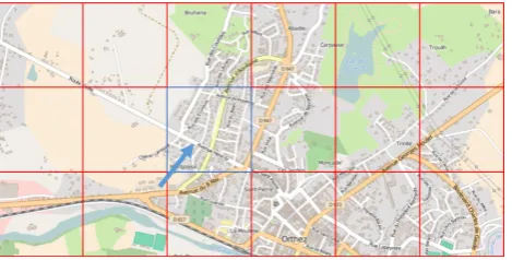
Automatic map generalization processes are computationally intensive, and they are most of the time unable to deal with the size of real region wide or countrywide geographical datasets. Distributing map generalization processes can help to both reduce the amount of data processed at once, and reduce the computation time by parallelizing the processes. But map generalization is a well-known holistic problem (Bundy et al 1995), as an automatic system needs to analyze the geographical context of any feature to decide what the best operation to apply is. If generalization is distributed, there is a major risk that quality might be damaged by hiding some parts of the geographical context. This problem is illustrated in Figure 1 with an example on road generalization, which needs some large con-text to decide what the important roads in an area are.
Some first proposals have been made to distribute generalization processes in the recent years (Chaudhry & Mackaness 2010), (Briat et al 2011), (Thiemann et al 2013), (Stanislawski et al 2015). But there is still no general guidelines on how to distribute a generalization process given the characteristics of the process and the dataset. That is why we propose to conduct some experiments to compare existing approaches, to analyze how much they can process large datasets without damaging the geographical context too much.
The second part of the paper describes the key problems of distributing generalization processes (partitioning, distributing context, parallelizing and reconciliation) and analyzes the approaches of each problem in the literature. Then, the third part describes how we conducted our experiments. The fourth part shows and discusses the results obtained and the fifth part draws some conclusions
Fig. 1. To generalize the roads of the center blue partition without surrounding context, it is not possible to consider the pointed road as the most important one, which it is considering this missing context (Source: @OpenStreetMap contributors).
2.
Key Problems to Distribute Generalization
Processes
2.1 Partitioning
The first step to distribute a generalization process is to partition a large dataset into parts that are small enough to be manageable by the process. Two main approaches exist and have been tried in the literature: regular partitioning and geographical partitioning.
Regular partitioning includes two methods, the use of a regular (often rectangular) grid, or the use of a quad tree. Regular grids have been used for land use generalization by (Thiemann et al 2011), and for most generic processes in (Briat et al 2011) and (Thiemann et al 2013). The size of the grid is adjusted based on the amount of data that can be found in one cell of the grid. The quad tree is a smarter version of the regular grid with smaller cells used in more dense areas, and (Briat et al 2011) showed that it can go faster than a simple regular grid.
would better capture the necessary geographical context while cutting data into small parts. A geographical partitioning can simply use features like administrative boundaries, as the US counties in (Briat et al 2011). (Chaudhry & Mackaness 2010) proposed a combination of a regular grid and a geographical partitioning based on geomorpho-logical regions, for DTM generalization. (Touya 2010) proposed a geographical partitioning based on main landscapes (urban, rurban, rural, mountain areas) with consideration for size (e.g. rural areas are cut by network elements and spaces without buildings to keep them small enough). (Thiemann et al 2013) proposes to cluster data based on proximity (Anders 2003) to create meaningful partitions.
2.2 Distribution of Geographical Context
Once a partitioning technique has been chosen, it is necessary to add a mechanism to restore some kind of geo-graphical context, at least for the features that are located near the boundary of a partition cell. The main proposition in the literature is to provide a buffer area around the partition where data is added for context, but not generalized by the process that handles the partition cell (Briat et al 2011), (Thiemann et al 2011). One difficulty here is to find the buffer size that gives enough context without making the partition cell too large to be processed. (Thiemann et al 2013) proposes a classification of the generalization operations that requires a large context, and the ones that can be triggered without any regard for the context. For instance, there is no need to look at the neighbors to simplify the shape of a building polygon, but network selection requires a large context (Fig. 1).
2.3 Parallelization
Different methods exist to parallelize the processes, even if the differences are more technical than conceptual. Parallelizing a process means that several nodes, i.e. cells of the partition, are processed in parallel by different computer cores, that can be in a same machine (Briat et al 2011), or not, and even in a machine cluster (Stanislawski et al 2015). There are some interesting details to tackle: for instance if the system allows multiple or single reads or writes on the dataset, or if some asynchronous mechanisms are used for adjacent partition cells (Briat et al 2011).
If the Map/Reduce framework is used for parallelization (Thiemann et al 2013), there are also implications for the way processes are implemented, and reimplementations might be required.
2.4 Reconciliation
The final issue is the reconciliation of the data processed in parallel, i.e. decide what to do if a feature has been included in several partition cells. (Thiemann et al 2013) calls this step composition. (Briat et al 2011) use an attribute field on features that says if it has been processed, and only the first processed partition is able to write the result on the feature at the reconciliation step. (Thiemann et al 2011) cut the features at the limits of the
partition and reconciliate by merging the cut parcels once generalized. However, cutting features is dangerous as shown in (Chaudhry & Mackaness 2008) with the example of Douglas & Peucker algorithm (Douglas & Peucker 1973) that fixes the initial/final vertices of the simplified lines, so more line cuts means more fixed points and less quality in generalization.
(Thiemann et al 2013) discusses three methods for reconciliation: selection (objects on the boundary of partition can be selected in only one partition cell), cut and merge, and match and adjust (objects are generalized in parallel and their new representation is matched and adjusted).
3.
Description of the Experiments
3.1 Hypotheses
Large datasets can cause two problems when generalized: too long processes and crashes because of the amount of data to process. The distribution techniques have to find the balance between computation time, the maximum amount of data processed at once, and the cartographic quality of the generalized map. We made four hypotheses about this balance between the three objectives of distribution:
− Optimizing time computation, or the amount of processed data does not optimize cartographic quality (H1).
− Regular partitioning is a better choice for non-contextual processes (H2).
− Geographical partitioning is better for contextual processes (H3).
− There is no generic best distribution method, it may depend on data types and processes (H4). − Distribution is not really platform dependent
(H5).
3.2 Case Study
We used a large dataset to experiment different distribution strategies, extracted from IGN (the French national mapping agency) topographic database that contains geographical data with a 1 meter geometric resolution. Data from Reunion Island was used as input data in our experiments. Reunion Island located in the Indian Ocean has been chosen mainly because of the variety of geographical features that it presents (dense cities, rural areas, dense hydrographic network, etc.), on an area large enough (2 512 km²) to cause issues for many non-distributed processes. We processed buildings, roads, rivers and coastlines from this dataset.
computer has 4 cores, so is able to run four processes in parallel. In order to test (H5), we also carried out experiments with the commercial platform 1Generalise from 1Spatial, that uses its own distributed system based on Oracle Weblogic Server.
For the remainder of the paper, we call a node a unitary element of the architecture able to run one process. In our architecture a node is one core of one of the available computers. We call a job the processing of a partition cell by one node.
For the purpose of the tests, two algorithms were chosen: the polyline simplification algorithm from (Visvalingam & Whyatt, 1993) and the building squaring algorithm currently developed at the IGN (Lokhat & Touya, 2016). The simplification algorithm is contextual because it was enhanced to avoid topological errors with the other lines of the dataset. The squaring algorithm is not contextual, each building being processed without any consideration for its neighbors. A high parameter value (2000 square meters) was chosen for the effective areas of the polyline simplification algorithm to highlight possible topological inconsistencies.
3.3 Description of the Experiments
Each distribution experiment was carried out with three different configurations of available nodes to distribute the process:
− A single computer with four nodes (a total of 4 nodes).
− Five computers, with a single node each (a total of 5 nodes).
− Five computers with four nodes each (a total of 20 nodes).
3.3.1 Experiments with Regular Partitions
We first carried out experiments with the simplest partitioning method, the rectangular grid. Two types of entities are treated using this partitioning solution, polylines (streams, roads and coastlines) and polygons (buildings). Regarding lines, the regular rectangular grid is implemented following two processing methods to handle context (Fig. 2a and b): one creating a buffer around each cell to provide a context for the simplification of polylines; the other cutting each lines according to the processed cell boundaries.
In the first method, it has been decided to use a buffer that includes each of the eight surrounding cells (Fig. 2a). The lines that intersect the buffer are loaded into memory, then their centers (located on the line) are calculated. If that point is inside the cell, the line will be processed, if not, it will be used as a context for the simplification algorithm in order to check any potential topology error caused by line intersections. If the center point of a line is located on the boundary of the cell, its identifier is stored and it will be treated afterwards, during the reconciliation stage. However, the error checking is done with the initial version of the lines, not the simplified ones, so intersections still might occur with the simplified lines. To avoid this problem, some asynchronous distribution should be used.
Fig. 2. Two strategies to handle context in a regular grid partition: (a) a buffer area around each cell; (b) cutting features at the edge of partition cells.
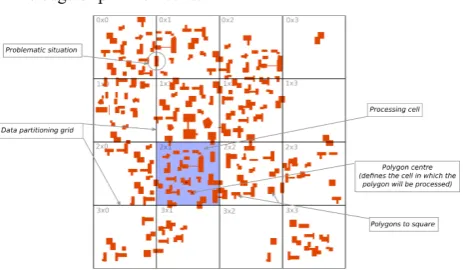
Fig. 3. Regular grid applied to building squaring: the building centroid is used to assign a building to a cell; buildings with the centroid on a partition edge are assigned to a final reconciliation job.
In the second method (Fig. 2b), all the new lines created during the splitting phase must keep an attribute indicating the initial line id. This allows the reconciliation stage to recreate initial lines by aggregating all the sections that have the same attribute.
Processing buildings using the regular grid is the simplest method to set up as the centroid of each entity defines in which cell it will be processed (Fig. 3). When a centroid is located on top of a cell's boundary, its identifier is stored and the building is processed at the end, during the reconciliation stage.
We also carried out experiments with a quad tree partition, but the results highlighted a performance issue in our implementation of the quad tree, making the quad tree less effective than the regular grid, which is not consistent with past research (Briat et al 2011). That is why we do not present any result with the quad tree in this paper.
3.3.2 Experiments with Geographical Partitions
cities, watershed extents or divisions based on the road network.
The partitioning according to the administrative boundaries as well as to the watershed extents is achieved following the same workflow as for the segmentation method. Lines are loaded, split, processed and reconciliated the same way, only the mask changes, from a regular grid it becomes a complex polygon geometry (which will cause some issues discussed in the last section).
The partitioning according to the road network was performed on the 1Generalise platform. It uses areas enclosed by road sections to create polygons which will be used as partitions. All small partitions formed inside the network are aggregated according to two main parameters: the maximum number of partitions to be merged and the maximum area allowed for a single partition. This method produces partitions which have various sizes but similar amount of data, producing partitions smaller in dense urban areas and larger ones in rural areas. This ensures that the processing time is fairly homogeneous across the partitions, for a more efficient load balancing across the grid of processing nodes. The processing then follows the same workflow as the previous method, cutting every line according to the boundaries of the partitions. Choosing the roads as partitioning features also helps keeping the number of split features down, and therefore limits the need for adding fixed points which are not ideal for the quality of the result.
4.
Results and Discussion
4.1 Operational Limitations
To properly understand the results, it is first mandatory to consider the material limitations as well as the other is-sues inherent to the method deployed. One has to take into consideration the memory limits of every node which happen when the partitions sent to the cluster hold too many entities. This phenomenon is observable when the regular grid used contains a small number of cells (Figure 4) or when the extent of the geographical object – such as the administrative areas or the watersheds – is too large (Figure 6); those can induce the presence of a large number of lines or buildings to be treated at once by a node. With more memory on each node, the balance between speed and cell size could be different.
Another limitation lies in the use of too many partitions that can lead to a significant growth in processing time. Indeed, in that case, the implemented distribution framework faces network congestions leading to failures with some jobs. This is not a major problem because it would be avoided by using a real grid architecture, and a more sophisticated distribution framework than JPPF. Finally, the hardware differences inside the cluster must be considered, one of the processor being weaker than the other four, the randomness of the node assignation can lead to different results with the use of the same architecture and the same number of partitions. We believe that this is not a standard configuration, and it
may cause biases preventing the comparisons between two strategies. So to over-come this limitation, we carried out each experiment several times and picked only the quickest results, i.e. the ones where the weak node of the grid did not handicap too much the process.
4.2 Regular Grid
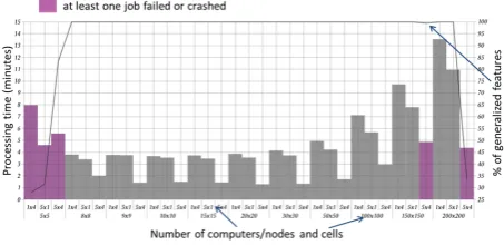
Concerning the results obtained with the regular rectangular grid, the first thing to notice is the overall lower speed of the method that cuts every line according to the cells boundaries. The duration is around 2 to 3 times higher when using the contextual method (Fig. 4).
Fig. 4. Results of the experiments with a regular grid for the generalization of rivers with the Visvalingam-Whyatt algorithm. The difference increases along with the number of nodes used in the cluster. That being mentioned, one must consider the quality of the data obtained as well. The results (one is showed in Fig. 4) show that there is a minimum processing time around 20x20 grids, which corresponds to 2.5x2.5 km cells on Reunion Island. We can also see that the architecture with five computers and four nodes by computer is the best one as predicted. The fall in the number of generalized features in the case with 200x200 cells and a 5x4 architecture illustrates the limitations of our framework, the high number of nodes to manage leading to network congestion and job failures. The method that splits the lines generates fixed points at every partition boundary, as extremities are kept in place during the simplification process. The contextual method produces data showing no trace of the partitioning stage as the algorithm considers the whole line while simplifying. Fig. 5 shows an example where cutting lines leads to a result very different from the buffer method output: the line is less simplified. The number of lines to reunite during the reconciliation stage then constitutes an indicator of the quality of the obtained data; the more lines needing to be aggregated, the worse the quality become. This proves that (H1) is true: the method that optimizes pro-cessing time and memory load does not provide the best cartographic results.
more building density crash because of the memory load. As shown by Briat et al (2011) a quad tree based method that makes more cells in dense areas would be the optimal solution.
Fig. 5. Differences in the cartographic output for Visvalingam-Whyatt simplification of rivers when using a buffer for context, or when cutting lines.
4.3 Geographical Partitioning
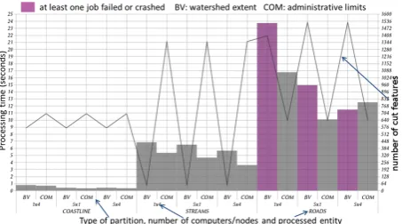
First, both the use of administrative boundaries and watersheds extent imply a significant limitation. The complexity of the geometries used to split lines is too important for the spatial query to be time-efficient. The difference observable with the use of a similar number of rectangular cells – which are simple-shaped polygons – is really noticeable and makes geographical partitioning ineffective for now. Another limitation is that the cells of the geo-graphical partitions we used were too big compared to the optimal cell size found with the previous experiments. Further experiments are clearly necessary to overcome these limitations that prevent us from asserting that (H3) is true, i.e. geographical partitioning is better for contextual generalization processes.
Nevertheless, our results give us hints on (H3). For instance, the use of watersheds as masks to split water streams, could be, if optimized, a way to enhance time-efficiency while preserving the quality of the data. Indeed, streams only cross watersheds boundaries at one point, the outlet, and the results have a much better quality (Fig. 6). Partitioning the dataset according to zones derived from the road network allows the same kind of principle as no road crosses another. The limitation for now lies in the fact that the whole network needs to be simplified before the creation of the actual partitions. This can induce some issues, particularly if the nodes composing the cluster have limited cache memory. The results obtained using this method show that the partitioning does not reflect on the quality of the simplified roads.
More generally, it might be difficult to assert that (H3) is true or false for all contextual processes. For instance, Fig. 5 shows that river streams simplification mostly requires the minimization of intersections between the partition cells and the streams, while building typification does require a view of the buildings neighborhoods to identify and preserve patterns, which cannot be guaranteed by a regular grid.
Fig. 6. Synthesis of the results for the simplification of lines using geographical partitioning based on watershed ex-tents and administrative limits.
These first results also suggest that (H4) might be true: the best distribution strategy depends on the feature types processed, and on the fact that the generalization process itself is more or less contextual. Apart from the current limitations we believe that the watershed based partitioning is the best when processing only rivers with a contextual algorithms such as simplification but also selection that is often carried out by watershed analysis (Stanislawski et al 2015).
The results obtained on the 1Generalise platform with the road network based partitioning show similar patterns between the number/size of cells and the processing time, with slight differences that might be due to differences in algorithm implementation and in the distribution architecture. One obvious difference lies in the fact that the pro-cessing nodes load the data in a local cache. This slows down the process, but removes the risk of failure due to lack of memory if the node is given a large area to process. However, we think that the patterns are similar enough to consider that (H5) is probably true: the platform differences are not significant compared to the differences due to partitioning and context handle methods.
5.
Conclusions and Future Work
more tests need to be run to see if this method proves to be quicker than the contextual one with a minor loss of quality. More generally, we plan to conduct much more experiments, with other partitioning and reconciliation methods, with generalization processes that require more context than the simplification algorithms, and with more robust distribution architectures.
For now, we only carried out experiments with the processing of a single algorithm on a single layer of the map, but a more realistic generalization processes needs to handle all the map layers and orchestrate the application of a large number of algorithms (Regnauld et al 2014). If the assumption that the optimal distribution strategy depends on the feature type and the amount of required context is true, a complete generalization process would require multiple distribution strategies, which might not be a feasible solution. In order to step up, and really make map generalization scalable, we have to develop global distribution models, as 1Generalise does, or maybe include the distribution issue into the generalization orchestration models.
6.
References
Anders, K.-H. (2003). A hierarchical graph clustering approach to find groups of objects. In Proceedings of 5th ICA Workshop on Progress in Automated Map Generalization, Paris, France.
Briat, M.-O., Monnot, J.-L., Punt, E. M. (2011). Scalability of contextual generalization processing using partitioning and paralleliza-tion. In Proceedings of 14th ICA Workshop on Generalisation and Multiple Representation, Paris, France.
Bucher, B., Brasebin, M., Buard, E., Grosso, E., Mustière, S., Perret, J. (2012). GeOxygene: Built on top of the expertness of the french NMA to host and share advanced GI science research results. In E. Bocher & M. Neteler (Eds.), Geospatial free and open source software in the 21st century (pp. 21–33). Berlin Heidelberg: Springer.
Bundy, G. L., Jones, C. B., Furse, E. (1995). Holistic generalization of large-scale cartographic data. In J.-C. Müller, J.-P. Lagrange, R. Weibel (Eds.), GIS and Generalisation: Methodology and Practice (pp. 106– 119). London: Taylor & Francis.
Chaudhry, O. Z., & Mackaness, W. A. (2008). Partitioning techniques to make manageable the generalisation of national spatial da-tasets. In ICA Workshop on Generalisation and Multiple Representation, Montpellier, France.
Chaudhry, O. Z., & Mackaness, W. A. (2010). DTM generalisation: Handling large volumes of data for Multi-Scale mapping. The Cartographic Journal 47(4), 360–370.
Douglas, D. H., & Peucker, T. K. (1973). Algorithms for the reduction of the number of points required to represent a digitized line or its caricature. Cartographica: The International Journal for Geographic Information and Geovisualization 10(2), 112–122.
Lokhat, I., & Touya, G. (2016). Enhancing Building Footprints with Squaring Operations, Journal of Spatial Information Science 13, 33–60.
Regnauld, N. (2014). 1Generalise: 1Spatial's new automatic generalisation platform. In Proceedings of 17th ICA Workshop on Gen-eralisation and Multiple Representation, Vienna, Austria.
Regnauld, N., Touya, G., Gould, N., Foerster, T. (2014). Process modelling, web services and geoprocessing. In D. Burghardt, C. Duchêne, W. Mackaness (Eds.), Abstracting Geographic Information in a Data Rich World (pp. 198–225). Berlin Heidelberg: Springer. Renard, J., Gaffuri, J., Duchêne, C. (2010). Capitalisation
problem in research - example of a new platform for generalisation: Car-tAGen. In Proceedings of 11th ICA Workshop on Generalisation and Multiple Representation, Zurich. ICA.
Stanislawski, L. V., Falgout, J., Buttenfield, B. P. (2015). Automated extraction of natural drainage density patterns for the contermi-nous United States through High-Performance computing. The Cartographic Journal 52(2), 185–192.
Thiemann, F., Warneke, H., Sester, M., Lipeck, U. (2011). A scalable approach for generalization of land cover data. In S. Geertman, W. Reinhardt, F. Toppen (Eds.), Advancing Geoinformation Science for a Changing World (pp. 399–420). Berlin, Heidelberg: Springer.
Thiemann, F., Werder, S., Globig, T., Sester, M. (2013). Investigations into partitioning of generalization processes in a distributed processing framework. In M. F. Buchroithner (Ed.), Proceedings of the 26th International Cartographic Conference, Dresden, Germany.
Touya, G. (2010). Relevant space partitioning for collaborative generalisation. In Proceedings of 12th ICA Workshop on Generalisa-tion and Multiple Representation, Zurich, Switzerland.