Hypergraph Optimization for Multi-Structural Geometric Model Fitting

(1)

The Thirty-Third AAAI Conference on Artificial Intelligence (AAAI-19)

Hypergraph Optimization for Multi-Structural Geometric Model Fitting

Shuyuan Lin,

1

_{Guobao Xiao,}

2

_{Yan Yan,}

1

_{David Suter,}

3

_{Hanzi Wang}

1∗

1_{Fujian Key Laboratory of Sensing and Computing for Smart City,} School of Information Science and Engineering, Xiamen University, China 2_{Fujian Provincial Key Laboratory of Information Processing and Intelligent Control,}

College of Computer and Control Engineering, Minjiang University, China 3_{School of Science, Edith Cowan University, Australia}

[email protected], [email protected],{yanyan, hanzi.wang}@xmu.edu.cn, [email protected]

Abstract

Recently, some hypergraph-based methods have been pro-posed to deal with the problem of model fitting in computer vision, mainly due to the superior capability of hypergraph to represent the complex relationship between data points. How-ever, a hypergraph becomes extremely complicated when the input data include a large number of data points (usually con-taminated with noises and outliers), which will significantly increase the computational burden. In order to overcome the above problem, we propose a novel hypergraph optimization based model fitting (HOMF) method to construct a simple but effective hypergraph. Specifically, HOMF includes two main parts: an adaptive inlier estimation algorithm for ver-tex optimization and an iterative hyperedge optimization al-gorithm for hyperedge optimization. The proposed method is highly efficient, and it can obtain accurate model fitting re-sults within a few iterations. Moreover, HOMF can then di-rectly apply spectral clustering, to achieve good fitting per-formance. Extensive experimental results show that HOMF outperforms several state-of-the-art model fitting methods on both synthetic data and real images, especially in sampling efficiency and in handling data with severe outliers.

Introduction

Robust fitting of geometric structures for multi-structural data contaminated with a number of outliers is one of the most important and challenging research tasks for many ap-plications of computer vision (Fischler and Bolles 1981), such as 2D line fitting (Li 2009), vanishing point detection (Tardif 2009), two-view segmentation (Magri and Fusiello 2014) and 3D-motion segmentation (Ochs and Brox 2012). The task of robust model fitting is to accurately and ef-ficiently recover meaningful structures from data. How-ever, data in many applications are often contaminated with noises and outliers, which makes the problem of model fit-ting challenging.

In the past few decades, the hypergraph representation has attracted much attention in many computer vision applica-tions (Parag and Elgammal 2011; Jain and Govindu 2013; Huang et al. 2016). A hypergraph modelling is an extended version of the traditional graph modelling. A graph mod-elling can be used to describe data through vertices and

∗

Corresponding author.

edges (an edge of a graph connects only two vertices), and a pairwise similarity measure (Saito, Mandic, and Suzuki 2018). Compared with a graph modelling, a hypergraph modelling can be used to effectively describe complex data relationship based on hyperedges (each of which may con-nect more than two vertices). For example, a probabilistic hypergraph method proposed by Huang et al. (Huang et al. 2010) establishes the relationship between the vertices and the hyperedge in terms of the local grouping information and the similarity in a probabilistic way. Generally speaking, the hypergraph modelling not only inherits the basic properties of the graph modelling, but also shows superior advantages over the graph modelling.

Recently, hypergraph analysis has been successfully ap-plied to robust model fitting and it has achieved promis-ing performance (Zhou, Huang, and Sch¨olkopf 2007; Agar-wal et al. 2005). The traditional hypergraph analysis usually considers the relationship between hyperedges and vertices. However, since data in practical tasks are often contaminated with noises and outliers, the traditional hypergraph-based methods suffer from two issues: 1) the hypergraph construc-tion becomes quite complex when data points are contami-nated with many outliers, and 2) a large number of hyper-edges generating from noisy vertices generally increase the computational cost. Therefore, it is quite important to opti-mize hypergraphs to reduce the computational complexity, which has not been well studied yet.

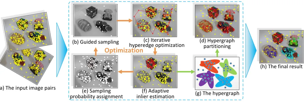
In this work, we propose a novel hypergraph optimiza-tion method (i.e., HOMF) for robust model fitting (as shown in Fig. 1) to overcome the above problems. HOMF can not only fit multi-structural data contaminated with both noises and outliers, but also effectively reduce the computational complexity. The main contributions of this paper are sum-marized as follows:

• We present an adaptive inlier estimation algorithm (AIE) based on the weighting scores of data points. As a result, AIE can effectively distinguish significant data points (i.e., inliers) from insignificant data points (i.e., outliers). • We develop an iterative hyperedge optimization algorithm

(2)

(b) Guided sampling (d) Hypergraph partitioning

(g) The hypergraph

(a) The input image pairs _{(f) Adaptive}

inlier estimation (e) Sampling

probability assignment

(h) The final result (c) Iterative

hyperedge optimization

Optimization

Figure 1: The overview of the proposed framework for two-view motion segmentation. (a) The outliers and the inliers are denoted in the yellow color. (b) Sampling points are marked with the white color. (c), (d) and (f) The sampled points are denoted in the red color and the other points are denoted in the yellow color. The red curves are denoted as the hyperedges. (e) Sampling points are marked with the white color and the red points surrounded by the white color means that they are assigned with a lower sampling probability. (g) The hypergraph with four hyperedges and some vertices. (h) The inliers belonging to different structures are denoted in the red, green, cyan and blue colors, respectively. The outliers are denoted in the yellow color.

same structure.

• We propose a novel hypergraph optimization method (HOMF) by taking advantage of IHO and AIE, which can be used for the guided sampling of different structures. Therefore, the proposed method is highly efficient and can efficiently obtain competitive fitting results.

The rest of the paper is organized as follows. Firstly, we review the related work. Then, we propose an adaptive inlier estimation algorithm and an iterative hyperedge optimiza-tion algorithm for hypergraph optimizaoptimiza-tion. Next, we report the experimental results obtained by our method and by sev-eral competing methods, on both synthetic data and real im-ages. Lastly, we draw conclusions.

Related Work

As the proposed method is closely related to scale estima-tion, guided sampling and hypergraph modelling, in this sec-tion, we briefly review work related to these.

Robust scale estimation plays a critical role for model fitting. A number of robust scale estimation methods (e.g., (Wang, Chin, and Suter 2012; Litman et al. 2015; Tiwari, Anand, and Mittal 2016)) have been proposed for the multi-structural fitting task. Wang et al. (Wang, Chin, and Suter 2012) propose the Iterative K-th Ordered Scale Estimator (IKOSE), which is one of the popular robust scale estima-tion methods due to its accuracy and efficiency. However, in practice, IKOSE is sensitive to the K-th sorted abso-lute residual. Tiwari et al. (Tiwari, Anand, and Mittal 2016) present the Density Preference Analysis (DPA) that esti-mates the scale of inlier noise by using linear extrapola-tion based residual density profile. But DPA overly relies on preference analysis, which focuses on the preference of data points to different models. In this paper, we propose a

novel robust adaptive scale estimator (i.e., AIE). The pro-posed AIE can efficiently estimate the scale of significant data points for heavily corrupted multi-structural data. As a result, the performance of model fitting can be significantly improved by using AIE.

Guided sampling can accelerate multi-stuctural data search by utilizing meta-information on the data distribu-tion (Pham et al. 2014; Tennakoon et al. 2018). The Ran-dom Cluster Model Simulated Annealing (RCMSA) (Pham et al. 2014) guides promising hypothesis generation by con-structing a weighted graph in a simulated annealing frame-work. However, the disadvantage of RCMSA is that it as-sumes spatial smoothness of the inliers, which is compu-tationally expensive and may not apply to particular situa-tions. The guided sampling method that is most closely re-lated to ours, cost-based sampling (CBS) (Tennakoon et al. 2018) uses a data sub-sampling strategy to generate the hy-potheses. Specifically, CBS employs aK-th order statistical cost function to improve the distribution of hypotheses. That method, however, relies on prior knowledge and the greedy algorithm. Unlike these previous works, we use AIE to iden-tify the insignificant data points (i.e., outliers) for guided sampling, which is more efficient for rapidly sampling min-imal subsets for different structures.

(3)

com-bination of the vertex labeling problem and the hyperedge estimation problem. However, it is challenging to solve both problems simultaneously. In this paper, we solve the hyper-graph optimization through an iterative updating strategy, by which the hypergraph can be optimized step by step dur-ing the iterative process. Then, spectral clusterdur-ing is used for partitioning the optimized hypergraph after hypergraph optimization.

Methodology

In this section, we describe the proposed HOMF, which takes advantage of an adaptive inlier estimation algorithm (AIE) and an iterative hyperedge optimization algorithm (IHO), for the geometric model fitting problem. Specifically, we first develop AIE to select the significant data points (i.e., inliers). Then we propose IHO for accelerating the optimiza-tion of initial hyperedges. Lastly, we present the complete HOMF method.

Adaptive Inlier Estimation

The inlier scale estimation plays a critical role in the hyper-graph optimization. However, most of the scale estimators need to manually choose a threshold for determining the number of model instances (Wang, Chin, and Suter 2012). To address the above problem, we propose AIE to adap-tively estimate the inlier noise scale. Specifically, AIE re-fines IKOSE (Wang, Chin, and Suter 2012) and kernel den-sity estimation (KDE) (Silverman 1986) to compute the weighting score of each data pointxifor a generated model

hypothesishusing the following equation:

ωi=

1

nb

EK rh_i/b

(1)

whereEK(·)is the popular Epanechnikov kernel function (Wand 1995);rh₌_{_rh

i}ni=1is the residual set between each data pointxiand the model hypothesish;nis the number

of data points. bis a bandwidth defined as follows (Wand 1995):

b=

"

7R₋1₁EK rh2dr

nR1

−1(r

h₎2_EK₍_rh₎_dr

#0.2

(2)

Inspired by (Sezgin and others 2004; Ferraz et al. 2007), we select significant data points by using a simple but ef-fective data driven thresholding technique. Given a set of data points X = {x1, x2, ..., xn} and the corresponding

squared weighting scoresw2₌_{_ω2

1, ω22, ..., ω2n}, we define

ξi = max{w2} −ω2i, which denotes the gap between the

squared weighting score of data pointsX and the squared weighting score of the data pointxifor the given model

hy-pothesish. Note that the logarithm is not meaningful when the gapξiis a negative value. The prior probabilityp(ξi)can

be computed asp(ξi) =ξi Pn_j₌₁ξj.

The entropy of the prior probability for all data points can be computed as follows:

Π =−

n

X

i=1

p(ξi) logp(ξi) (3)

Algorithm 1:The adaptive inlier estimation (AIE) Input:The residuals (to a hypothesis)rhand the

number of data pointsn. Output:The significant data pointsϑ∗.

1 Compute the bandwidthbof the kernel density function

by Eq. (2).

2 Estimate the weighting score for each data point by Eq.

(1).

3 Calculate the entropyΠbased on the set of the

weighting scores by Eq. (3).

4 Select the significant data points (i.e., inliers)ϑ∗by Eq.

(4).

The entropy is chosen as the threshold to distinguish the significant data points from the insignificant data points, as follows:

ϑ∗=

xi

−logp(ξi)>Π

(4)

Here, we use information theory (Wang, Chin, and Suter 2012) in Eq. (4) to select the significant data points and reject the other insignificant data points. It is worth point-ing out that the difference between (Wang, Chin, and Suter 2012) and the proposed is that AIE can adaptively choose the number of significant data points independent of theK -th sorted absolute residual.

Hypergraph Optimization for Model Fitting

In this paper, a hypergraph is defined as G= (V,E,W), which includes the vertex set V={v1, v2, ..., vn}, the

hy-peredge set E={e1, e2, ..., em}, and the weight setW =

{ω1, ω2, ..., ωn}, wherenandmare respectively the

num-ber of vertices and the numnum-ber of the hyperedges. Each ver-tex is assigned a weighting scoreωi(see Sec. Adaptive Inlier

Algorithm 2: The iterative hyperedge optimization (IHO)

Input:The initial hyperedgeE(e), the vertices V={vi}

n

i=1, the minimum tolerable sizeq, the higher than minimal subsetland the number of iterationsTmax.

Output:The optimized hyperedgeE(ˆ et).

1 fort=1toTmaxdo

2 Calculate the residualrhbetween the hyperedge

and the vertices.

3 Estimate the weighting scoreωof each element in

rh_{by Eq. (1) to obtain the weighting score set}_w t.

4 Sortwtin the ascending order to obtain the

permutationw˜t.

5 Generate a new hyperedgeEˆ(et)by refitting the

vertices corresponding to the[ ˜wt]q_q₋_l.

6 EvaluateQein Eq. (6).

7 ifQe== 1thenbreak;

(4)

Estimation). The hypergraph modellingGis an extension of an ordinary graph modelling, where the hyperedgeemight connect more than two vertices, to also include weights.

In our hypergraph construction, each vertex is defined as a data point and each hyperedge corresponds to a model hy-pothesis. We construct the hyperedge of hypergraph based on the higher than minimal subset sampling (HMSS) algo-rithm due to its good accuracy and efficiency, which has been demonstrated in (Tennakoon et al. 2016).

Similar to (Govindu 2005; Ochs and Brox 2012; Ten-nakoon et al. 2018), in order to make the hypergraph opti-mization tractable, we decompose the hypergraph by mul-tiplying the pairwise affinity matrix H with its transpose. Each column of the affinity matrixH, which is obtained by encoding more than two vertices as a subset, corresponds to the hyperedge. The affinity matrixHcharacterizes the rela-tionships between hyperedgesEand verticesV. Specifically, the simple version of the hypergraphG∗ is represented as follows:

G∗=HHT=

m

X

i

exp−2σwi2

T

(5)

whereexp(·)_{is the exponential map.}_w

iis the set of

weight-ing scores, which is computed by Eq. (1) between the hy-peredgeeiand verticesV.σis a normalization constant.[·]T

is the transpose of[·].mis the number of hyperedges. The hypergraphG∗contains many redundant vertices and hyper-edges, which will lead to the high computational complexity. Thus, it needs to be optimized step by step during the sub-sequent iterative updating process (see Alg. 2). The detail of the hypergraph optimization is given as follows:

Firstly, we generate a new model hypothesis using the ran-dom sampling with HMSS (Tennakoon et al. 2016) to add an initial hyperedge in the hypergraph.

Then, we estimate the set of weighting scoreswithat will

be sorted as an ordered weighting scores permutationw˜i.

Thirdly, we adopt an iterative algorithm to effectively and efficiently optimize the hypergraph. Similar to (Tennakoon et al. 2016), we determine whether the hypergraph construc-tion process converges based on the last three iteraconstruc-tions. However, the difference between the proposed method and (Tennakoon et al. 2016) is that we use the weighting scores of the vertices as condition for the ‘exiting criterion’, whose advantage is that it can reduce the sensitivity to residuals. In contrast, (Tennakoon et al. 2016) uses the residual of data points as conditions. Specifically, the ‘exiting criterion’Qe

is formulated as follows:

Qe=

ωq,t2 < q

X

j=q−l

ωj,t2 −1

∧

ω2q,t< q

X

j=q−l

ω2j,t−2

(6)

wherelandqare respectively the higher than minimal sub-set (i.e., the minimal subsub-setp+2) and the minimum tolerable size of the same structure (ql, in our experiment, we set theqto be0.1×n).tdenotes the number of current iteration.

ωq,tis the weighting score in current iterationtwith respect

to the minimum tolerable sizeq. The results obtained from the last three iterations (i.e.,t,t−1andt−2 iterations) are more likely to belong to the same structure (Tennakoon

Algorithm 3:The hypergraph optimization based model fitting (HOMF) method

Input:A set of data pointsX={xi}ni=1, the number of model hypothesismand the number of structuresc.

Output:The model instances and the hyperedges.

1 Initialize the sampling probabilityP ={ρi}ni=1of all data points to 1.

2 Generate a model hypothesishby random sampling.

3 Construct a hypergraphG∗based on the generated

model hypothesish.

4 forj=1tomdo

5 ifj>1then

6 Generate a new model hypothesishjaccording

to the sampling probabilityPand add a hyperedgeE(ej)according tohjinG∗.

7 end

8 Generate an optimized hyperedgeE(ˆe_j)by Alg. 2. 9 Calculate the residualrh

j between the vertices and

optimized hyperedgeE(ˆej).

10 Optimize the vertices connected to the optimized hyperedgeE(ˆ ej)using AIE by Alg. 1.

11 Update the sampling probability of the verticesP.

12 end

13 Segment the hypergraph by spectral clustering to obtain

the model instances and the hyperedges.

et al. 2016). The above steps can quickly generate the op-timized hyperedge but cannot effectively remove some re-dundant vertices (i.e., insignificant data points), which will affect the following sampling procedure (guided sampling). Hence, we use AIE (see Sec. Adaptive Inlier Estimation) for estimating the vertices (corresponding to the significant data points) of optimized hyperedge to solve this problem.

After that, the weighting scores of vertices correspond-ing to the significant data points are selected to optimize the affinity matrixHand the vertices corresponding to the in-significant data points are assigned a higher sampling prob-ability. Specifically, the sampling probability of the signifi-cant vertices is gradually increased about 2-10 times, while the sampling probability of the other vertices is gradually reduced about 2-10 times during each update process.

Finally, these vertices (corresponding to the insignificant data points) will guide the following sampling procedure, which will focus on sampling for different structures. This way can effectively improve the contribution of vertices cor-responding to the insignificant data points for hypergraph optimization.

(5)

The Complete Method

In the previous subsections, we gave all the components of the proposed HOMF method. Now we describe the complete algorithm in Alg. 3. Firstly, random sampling is used for generating an initial hypergraph. Then, IHO is employed to accelerate the optimization of hyperedges. The vertices (cor-responding to the significant data points) of the optimized hyperedges are then estimated using AIE. Secondly, we as-sign a lower sampling probability for each vertex (corre-sponding to the significant data point) and a higher sampling probability for other vertices (corresponding to the insignif-icant data points). In this way, the vertices corresponding to the significant data points can be selected to reduce the com-putational complexity and the vertices corresponding to the insignificant data points can be used for guided sampling, which in turn enhances hypergraph construction. This opti-mization process is performed iteratively until the ‘exiting criterion’ is reached (or the fixed number of iterations is reached). Fortunately, the ‘exiting criterion’ causes the pro-posed method only perform only a few iterations. Lastly, spectral clustering is applied to obtain the model instances and the hyperedges.

Experiments

In this section, we firstly evaluate the performance on syn-thetic data of AIE compared several robust scale estimation methods including the median (MED), the median abso-lute deviation (MAD), KOSE (Lee, Meer, and Park 1998), IKOSE (Wang, Chin, and Suter 2012), AIKOSE (Wang, Cai, and Tang 2013) and DPA (Tiwari, Anand, and Mit-tal 2016). Then we compare the performance on real im-ages of proposed HOMF with several state-of-the-art model fitting methods including CBS (Tennakoon et al. 2018), MSHF (Wang et al. 2018), RPA (Magri and Fusiello 2015), RCMSA (Pham et al. 2014) and UHG (Lai et al. 2017). All experimental results are obtained by running 50 times.

Experiments on Scale Estimation (Synthetic Data)

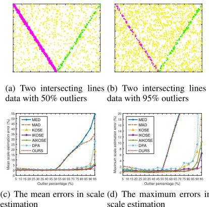
The experiments undertaken in this section are described as follows. Two intersecting lines are generated lying on a plane that contains a total number of 2000 data points. The number of the data points of the left line is decreased from 1900 to 100, which means that the outlier ratio is gradually increased from 5% to 95%. Meanwhile, the right line is hold fixed at 100 data points. We report the standard variances, the mean scale estimation errors, the median scale estima-tion errors and the maximum scale estimaestima-tion errors in Ta-ble 1. We then respectively display the data points with the outlier percentages on 50% and 95% in Fig. 2 (a) and 2 (b), and the mean and maximum errors in Fig. 2 (d) and 2 (e). Similar to (Wang, Chin, and Suter 2012), we use Eq. (7) to compute the scale of inlier noise.

sh=|˜rκ|

.

Φ−1

_{1 +}_κ/_n_˜

2

(7)

wheren˜ is the number of significant data pointsϑ∗, which are selected according to the entropy. Then, the scale esti-mation is measured through the following (Wang, Chin, and

(a) Two intersecting lines data with 50% outliers

(b) Two intersecting lines data with 95% outliers

5 10 15 20 25 30 35 40 45 50 55 60 65 70 75 80 85 90 95

Outlier percentage (%)

-5 0 5 10 15 20 25 30 35 40 45 50 55

Mean scale estimation error (%)

MED MAD KOSE IKOSE AIKOSE DPA OURS

(c) The mean errors in scale estimation

5 10 15 20 25 30 35 40 45 50 55 60 65 70 75 80 85 90 95 Outlier percentage (%) 0

2 4 6 8 10 12 14 16 18 20

Maximum scale estimation error (%)

(d) The maximum errors in scale estimation

Figure 2: Comparisons of the performance obtained by seven methods for scale estimation on synthetic data with 5%-95% outliers. (a) and (b) are respectively the data points with the outlier percentages on 50% and 95%. (c) and (d) display the mean and maximum errors among the scale esti-mation, which are obtained from all the competing methods.

Table 1: Quantitative evaluation of the seven inlier scale es-timation methods on synthetic data (the best results are bold-faced).

Std. 16.43 12.01 4.26 1.03 1.48 6.26 0.40

Mean 12.13 10.19 2.04 0.74 0.68 2.59 0.32

Med. 0.83 2.04 0.59 0.44 0.19 0.74 0.16

Max. 54.02 35.04 18.40 4.84 6.32 28.05 1.59

Suter 2012):

Λ(se, st) = max

s_e

st

,st

se

−1 (8)

wherestis the true scale, andseis the estimated scale. As

displayed in Table 1 and Fig. 2, all the scale estimation meth-ods can work well when the outlier ratio is less than 50%. However, MED and MAD fail to estimate the scales when the outlier ratio is larger than 50%. The error of KOSE be-gins to increase when the outlier ratio is larger than 65%, but is still better than MED and MAD. KOSE and DPA be-come gradually worse when the outlier ratio is larger than 75%. IKOSE and AIKOSE can also achieve better results than other methods when the outlier ratio is larger than 90%. Among all the competing methods, the proposed method is able to achieve the best results, since it can adaptively esti-mate the inlier scale.

Experiments on Segmentation (Real Images)

(6)

(a) Biscuitbookbox (b) Breadcartoychips (c) Breadcubechips

(d) Cubechips (e) Cubetoy (f) Cube

Figure 3: Some results obtained by the proposed method on six image pairs for two-view motion segmentation (only one view is shown).

data from the AdelaideRMF datasets (Wong et al. 2011) for two-view motion segmentation and multi-homography seg-mentation, respectively. Then, the average misclassification rates and the CPU time (including sampling and fitting) are both reported in Table 2 and Table 3 for the two tasks, re-spectively. The misclassification rate is adopted to measure the performance of these methods. It is defined as (Mittal, Anand, and Meer 2012):

error=number of misclassified points

total number of points ×100%. (9)

The sampling frequency has a significant influence on sampling time. More sampled minimal subsets can usually achieve better segmentation results. In fairness to the best accuracy of all the competing methods in our experiment, we also analyze the influence of sampling frequency on the six methods, where the number of minimal subsets is grad-ually increased from 100 to 20000 times on both fundamen-tal matrix estimation and homography estimation. We repeat the experiments 50 times and show the mean results in Fig. 4. Note that RPA fails to obtain the fitting results on a num-ber of image pairs, when the sampling frequency is 100 and 500 times. Therefore, the results on these two sampling fre-quencies are not given. As shown in Fig. 4, the experimen-tal results show that CBS, MSHF, RPA, RCMSA and UHG achieve the minimum average misclassification rates at 500, 20000, 5000, 10000 and 1000 times, respectively, and these values will be used in all experiments. The proposed method obtains the stable average misclassification rates due to the IHO, the AIE and the guided sampling. Therefore, we fix the sampling frequency to 200 times for the proposed method in the experiments.

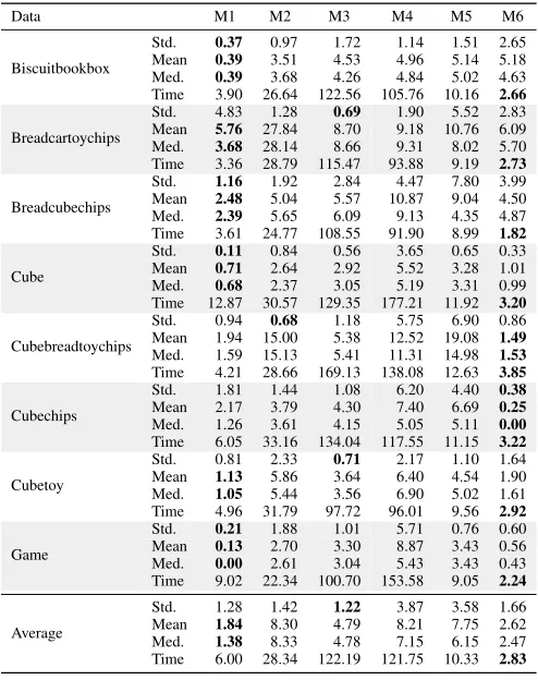
Two-view Motion Segmentation In this section, we eval-uate the partitioning capability of the six competing methods to identify two-view motion segmentation. From the data reported in Table 2 and Fig. 3 (except for Cubebreadtoy-chips and Game due to the space limit), we can see that our method achieves the fastest running time (in seconds)

http://cs.adelaide.edu.au/hwong/doku.php?id=data

100 500 1000 5000 10000 20000 The number of sampled minimal subsets 0

5 10 15

Average misclassification rate (%)

CBS MSHF RPA RCMSA UHG OURS

Figure 4: The average results are obtained by the six meth-ods on a different number of sampled minimal subsets from the AdelaideRMF datasets.

among all the competing methods. Although the segmenta-tion accuracy of HOMF is slightly lower than CBS, it has significantly improved computational speed over CBS for all the representative image pairs. CBS achieves the low-est average misclassification rates due to thekth-order cost function and the greedy algorithm. RPA achieves the third lowest average misclassification rates, however it takes more time to sample the minimal subset than other methods. UHG

Table 2: Misclassification rates (in percentage) and the CPU time (in seconds) for two-view motion segmentation on six methods (the best results are boldfaced).

Data M1 M2 M3 M4 M5 M6

Std. 0.37 0.97 1.72 1.14 1.51 2.65 Mean 0.39 3.51 4.53 4.96 5.14 5.18 Med. 0.39 3.68 4.26 4.84 5.02 4.63 Biscuitbookbox

Time 3.90 26.64 122.56 105.76 10.16 2.66

Std. 4.83 1.28 0.69 1.90 5.52 2.83 Mean 5.76 27.84 8.70 9.18 10.76 6.09 Med. 3.68 28.14 8.66 9.31 8.02 5.70 Breadcartoychips

Time 3.36 28.79 115.47 93.88 9.19 2.73

Std. 1.16 1.92 2.84 4.47 7.80 3.99 Mean 2.48 5.04 5.57 10.87 9.04 4.50 Med. 2.39 5.65 6.09 9.13 4.35 4.87 Breadcubechips

Time 3.61 24.77 108.55 91.90 8.99 1.82

Std. 0.11 0.84 0.56 3.65 0.65 0.33 Mean 0.71 2.64 2.92 5.52 3.28 1.01 Med. 0.68 2.37 3.05 5.19 3.31 0.99 Cube

Time 12.87 30.57 129.35 177.21 11.92 3.20

Std. 0.94 0.68 1.18 5.75 6.90 0.86 Mean 1.94 15.00 5.38 12.52 19.08 1.49

Med. 1.59 15.13 5.41 11.31 14.98 1.53

Cubebreadtoychips

Time 4.21 28.66 169.13 138.08 12.63 3.85

Std. 1.81 1.44 1.08 6.20 4.40 0.38

Mean 2.17 3.79 4.30 7.40 6.69 0.25

Med. 1.26 3.61 4.15 5.05 5.11 0.00

Cubechips

Time 6.05 33.16 134.04 117.55 11.15 3.22

Std. 0.81 2.33 0.71 2.17 1.10 1.64 Mean 1.13 5.86 3.64 6.40 4.54 1.90 Med. 1.05 5.44 3.56 6.90 5.02 1.61 Cubetoy

Time 4.96 31.79 97.72 96.01 9.56 2.92

Std. 0.21 1.88 1.01 5.71 0.76 0.60 Mean 0.13 2.70 3.30 8.87 3.43 0.56 Med. 0.00 2.61 3.04 5.43 3.43 0.43 Game

Time 9.02 22.34 100.70 153.58 9.05 2.24

Std. 1.28 1.42 1.22 3.87 3.58 1.66 Mean 1.84 8.30 4.79 8.21 7.75 2.62 Med. 1.38 8.33 4.78 7.15 6.15 2.47 Average

Time 6.00 28.34 122.19 121.75 10.33 2.83

(7)

achieves relatively good performance due to the promis-ing hypothesis generation which is effectively accelerated. RCMSA and MSHF obtain similar average misclassification rates, but MSHF runs much faster than RCMSA. This is be-cause that RCMSA employs a simulated annealing frame-work, which is time-consuming. In contrast, our method achieves good average misclassification rates (only slightly worse than CBS) with low computational cost. Therefore, our method achieves good tradeoff between the segmenta-tion performance and running time.

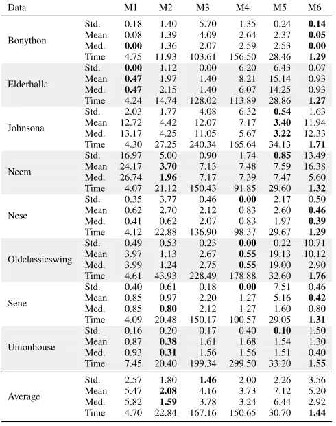
Multi-homography Segmentation In this section, we also evaluate the performance of the six competing meth-ods for multi-homography segmentation. From the data re-ported in Table 3 and Fig. 5 (omitting Oldclassicswing and Unionhouse due to the space limit), we can see that our method can more efficiently recover the real plane structure on multi-homography segmentation. Our method achieves superior speed (in seconds) over the other com-peting methods, although the average misclassification rates are higher than MSHF and RCMSA. This is because that the lower number of sampled minimal subsets leads to fail-ure of multi-structural data with high complexity (e.g., Fig. 5 (c)). MSHF achieves the lowest average misclassification

Table 3: Misclassification rates (in percentage) and the CPU time (in seconds) for multi-homography segmentation on six methods (the best results are boldfaced).

Data M1 M2 M3 M4 M5 M6

Std. 0.18 1.40 5.70 1.35 0.24 0.14

Mean 0.08 1.39 4.09 2.64 2.37 0.05

Med. 0.00 1.36 2.07 2.59 2.53 0.00

Bonython

Time 4.75 11.93 103.61 156.50 28.46 1.29

Std. 0.00 1.12 0.00 6.20 6.43 0.07 Mean 0.47 1.97 1.40 8.21 15.14 0.93 Med. 0.47 2.15 1.40 6.07 14.25 0.93 Elderhalla

Time 4.24 14.74 128.02 113.89 28.86 1.27

Std. 2.03 1.77 4.08 6.32 0.54 1.63 Mean 12.72 4.42 12.07 7.17 3.40 11.94 Med. 13.17 4.25 11.05 5.67 3.22 12.33 Johnsona

Time 4.30 27.25 240.34 165.64 34.13 1.71

Std. 16.97 5.00 0.90 1.74 0.85 13.49 Mean 24.17 3.70 7.13 7.48 7.59 16.38 Med. 26.74 1.96 7.17 7.39 7.47 5.60 Neem

Time 4.07 21.12 150.43 91.85 29.60 1.32

Std. 0.35 3.77 0.46 0.00 2.17 0.50 Mean 0.62 2.70 2.12 0.83 2.60 0.46

Med. 0.41 0.62 2.07 0.83 1.97 0.39

Nese

Time 4.12 22.88 136.90 98.37 29.67 1.29

Std. 0.49 0.53 0.23 0.00 0.22 10.71 Mean 3.97 1.13 2.67 0.55 19.13 10.12 Med. 3.99 1.24 2.75 0.55 19.00 2.90 Oldclassicswing

Time 4.61 43.93 228.49 178.88 32.60 1.76

Std. 0.40 0.61 0.18 0.00 7.51 0.46 Mean 0.85 0.97 2.20 1.27 5.16 0.42

Med. 0.85 0.80 2.12 1.27 1.60 0.80 Sene

Time 4.09 20.48 150.17 100.57 29.05 1.31

Std. 0.16 0.20 0.17 0.40 0.10 1.50 Mean 0.87 0.38 1.61 1.68 1.54 1.30 Med. 0.93 0.31 1.56 1.56 1.51 0.40 Unionhouse

Time 7.45 20.40 199.34 299.50 33.20 1.55

Std. 2.57 1.80 1.46 2.00 2.26 3.56 Mean 5.47 2.08 4.16 3.73 7.12 5.20 Med. 5.82 1.59 3.78 3.24 6.44 2.92 Average

Time 4.70 22.84 167.16 150.65 30.70 1.44

(M1-CBS; M2-MSHF; M3-RPA; M4-RCMSA; M5-UHG; M6-HOMF.)

(a) Bonython (b) Elderhalla (c) Johnsona

(d) Neem (e) Nese (f) Sene

Figure 5: Some results obtained by the proposed method on six image pairs for multi-homography segmentation (only one view is shown).

rate (in percentage) among all the competing methods be-cause of the effectiveness of the constructed hypergraph. However, the running time of MSHF is slower than our method. Both RCMSA and RPA achieve similar results in accuracy and performance, but obtain slow speeds due to the time-consuming sampling process. CBS fails in the im-age pairs due to the loss of useful information during the data sub-sampling strategy. UHG does not achieve reliable fitting performance since it selects the model instance by using T-Linkage (Magri and Fusiello 2014). Nevertheless, the experimental results show that HOMF performs faster than the other five competing methods in practice, includ-ing samplinclud-ing and fittinclud-ing time. Experimental results show that our method can segment multi-structural data with outliers quickly and efficiently.

Conclusion

(8)

Acknowledgments. We would like to thank anonymous reviewers for their suggestions. This work was supported by the National Natural Science Foundation of China un-der Grants U1605252, 61702431, 61472334, 61571379 and 61872307. David Suter acknowledges funding under ARC DP160103490.

References

Agarwal, S.; Lim, J.; Zelnik-Manor, L.; Perona, P.; Krieg-man, D.; and Belongie, S. 2005. Beyond pairwise clustering. InCVPR, 838–845.

Ferraz, L.; Felip, R.; Mart´ınez, B.; and Binefa, X. 2007. A density-based data reduction algorithm for robust estima-tors. InPRIA, 355–362.

Fischler, M. A., and Bolles, R. C. 1981. Random sample consensus: a paradigm for model fitting with applications to image analysis and automated cartography. Commun. of the ACM24(6):381–395.

Govindu, V. M. 2005. A tensor decomposition for geometric grouping and segmentation. InCVPR, 1150–1157.

Huang, Y.; Liu, Q.; Zhang, S.; and Metaxas, D. N. 2010. Im-age retrieval via probabilistic hypergraph ranking. InCVPR, 3376–3383.

Huang, S.; Yang, D.; Liu, B.; and Zhang, X. 2016. Regression-based hypergraph learning for image clustering and classification.arXiv preprint arXiv:1603.04150. Jain, S., and Govindu, V. M. 2013. Efficient higher-order clustering on the grassmann manifold. In CVPR, 3511– 3518.

Lai, T.; Wang, H.; Yan, Y.; and Zhang, L. 2017. A unified hypothesis generation framework for multi-structure model fitting. Neurocomputing222:144–154.

Lee, K.-M.; Meer, P.; and Park, R.-H. 1998. Robust adap-tive segmentation of range images. IEEE Trans. PAMI

20(2):200–205.

Li, H. 2009. Consensus set maximization with guaranteed global optimality for robust geometry estimation. InICCV, 1074–1080.

Litman, R.; Korman, S.; Bronstein, A.; and Avidan, S. 2015. Inverting ransac: Global model detection via inlier rate esti-mation. InCVPR, 5243–5251.

Magri, L., and Fusiello, A. 2014. T-linkage: A continuous relaxation of j-linkage for multi-model fitting. In CVPR, 3954–3961.

Magri, L., and Fusiello, A. 2015. Robust multiple model fitting with preference analysis and low-rank approximation. InBMVC, 12.

Mittal, S.; Anand, S.; and Meer, P. 2012. General-ized projection-based m-estimator. IEEE Trans. PAMI

34(12):2351–2364.

Ochs, P., and Brox, T. 2012. Higher order motion models and spectral clustering. InCVPR, 614–621.

Parag, T., and Elgammal, A. 2011. Supervised hypergraph labeling. InCVPR, 2289–2296.

Pham, T. T.; Chin, T.-J.; Yu, J.; and Suter, D. 2014. The ran-dom cluster model for robust geometric fitting.IEEE Trans. PAMI36(8):1658–1671.

Saito, S.; Mandic, D. P.; and Suzuki, H. 2018. Hypergraph

p-laplacian: A differential geometry view. InAAAI, 3984– 3991.

Sezgin, M., et al. 2004. Survey over image thresholding techniques and quantitative performance evaluation. JEI

13(1):146–168.

Silverman, B. W. 1986.Density estimation for statistics and data analysis, volume 26. CRC press.

Tardif, J.-P. 2009. Non-iterative approach for fast and accu-rate vanishing point detection. InICCV, 1250–1257. Tennakoon, R. B.; Bab-Hadiashar, A.; Cao, Z.; Hosein-nezhad, R.; and Suter, D. 2016. Robust model fitting using higher than minimal subset sampling. IEEE Trans. PAMI

38(2):350–362.

Tennakoon, R.; Sadri, A.; Hoseinnezhad, R.; and Bab-Hadiashar, A. 2018. Effective sampling: Fast segmentation using robust geometric model fitting. IEEE Trans. on IP

27(9):4182–4194.

Tiwari, L.; Anand, S.; and Mittal, S. 2016. Robust multi-model fitting using density and preference analysis. In

ACCV, 308–323.

Wand, M. 1995. Mc: Jones, kernel smoothing.

Wang, H.; Xiao, G.; Yan, Y.; and Suter, D. 2018. Searching for representative modes on hypergraphs for robust geomet-ric model fitting. IEEE Trans. PAMI.

Wang, H.; Cai, J.; and Tang, J. 2013. Amsac: An adaptive robust estimator for model fitting. InICIP, 305–309. Wang, H.; Chin, T.-J.; and Suter, D. 2012. Simultaneously fitting and segmenting multiple-structure data with outliers.

IEEE Trans. PAMI34(6):1177–1192.

Wong, H. S.; Chin, T.-J.; Yu, J.; and Suter, D. 2011. Dy-namic and hierarchical multi-structure geometric model fit-ting. InCVPR, 1044–1051.

Zhou, D.; Huang, J.; and Sch¨olkopf, B. 2007. Learning with hypergraphs: Clustering, classification, and embedding. In