Convex quadratic optimization based on
generator matrix in credit risk transfer
process
Liping Zhang
♯1♯School of Information Science and Technology, Department of Mathematics, Jinan
University, Guangzhou, Guangdong, 510632, PR of China
Abstract. In this paper, the generator matrix is calculated based on the grade transfer
matrix over a period of time in the quantitative analysis of credit risk, which has become one
of the hot issues that many scholars pay attention to and study.From the mathematical model
point of view combined with the actual situation, the calculation of the generated matrix can
be regarded as optimization problems of the matrix logarithm. This article is based on Prof
Kreinin and Prof Sidelnikova’s classical optimization model, and we use the combination model
of Markov chain and the effective set method of convex quadratic optimization to solve the
problem. We mainly make the feasible domain satisfy the applicable conditions by reducing
dimensions and correcting variables and theoretically verify the convergence and feasibility of
the optimization system. Meanwhile, we verify the data published by Standard and Poor’s
Credit Review by Matlab.
Keywords. credit risk, convex quadratic optimization, effective set method, generator
matrix, Markov chain
1. Introduction
The JLT model is an important model in the quantitative analysis of credit risk. It
constructs a non-timed continuous chain to portray the process of change of the credit rating
in the risk neutrality measurement space by some market data, such as the country Debt,
corporate bond and other prices. An important step in implementing the JLT model is to
assume that the credit-level transfer process is a continuous Markov chain in the real-world
measurement space. And how to calculate a generator matrix based on the credit-level transfer
matrix published by the credit rating agency for a period of time? Expressed in mathematical
language, given the transition matrixP(0, T) for a given time period [0,T] to calculate a matrix
matrix), so that eQT is as close as possible to P(0, T). [2] and [5] proposed a method to solve this problem: first calculate the matrix logP(0, T), and then modify logP(0, T)/T to a matrix Q that satisfies the properties of the generator matrix. This article has made two improvements to the methods in [2] and [5]:
First, when T is small, logP(0, T) has a strong diagonal dominance, then ∥logP(0, T)∥ is small. We use the inverse scaling and squaring algorithm with specified relative precision
to calculate the logarithmic matrix, so that the calculated value guarantees a certain relative
precision.
Second, it is well known that the results obtained directly through the matrix logarithm
operation do not satisfy the nature of the generation matrix of the credit level transfer in the
real world. It is pointed out in [10] that more accurate prediction estimates can be obtained
by optimization methods. In this paper, we fully consider this point when doing matrix
correction. The properties of the generator matrix are taken as constraints, and logP(0, T)/T
is corrected to the matrix Qby solving the linear optimization problem.
2. Preliminary
In this chapter we will introduce the relevant knowledge of continuous time Markov chain
and convex quadratic optimization, which will lay the foundation for the following
discus-sion[3,16].
2.1 Continuous time Markov chain
The random process{Xn, n∈N}(whereN represents the set of indicators of time) is called
the Markov process[7,8].
If the conditional probability satisfies the Markov property, that is, ∀t, a positive integer
n, and an arbitrary sequencet0, t1,· · ·, tn that satisfies t0 < t1 <· · ·< tn < t, the following
equation holds:
P{Xt≤x|Xt0 =x0, Xt1 =x1,· · · , Xtn =xn}=P{Xt≤x|Xtn =xn}.
It can be obtained from the above formula that the Markov process is a process in which
future state changes are only related to the current state, and are independent of the previous
If the state space of a Markov process is discrete, then this Markov process is called the
Markov chain.
If the indicator set T is continuous, it is called a continuous time Markov chain. In this case, the Markov property is expressed as: ∀n and an arbitrary sequence t0, t1,· · ·, tn, tn+1
that satisfies t0 < t1 <· · ·< tn< tn+1, The following equation holds:
P{Xtn+1 =xn+1|Xt0 =x0, Xt1 =x1,· · · , Xtn =xn}=P{Xtn+1 =xn+1|Xtn =xn}.
In the continuous Markov chain, pij(s, t) =P{Xt= j|Xs = i} represents the probability
of the time point t is in the state j under the condition of the time point s is in the state
i, which is called the transition probability equation of the state i to j. Transfer matrix[10]
P(s, t) = (pij(s, t)) satisfies:
P(s, t)≥0; P(s, t)e=e, (2.1)
whereerepresents unit vector, that ise= [1,1,· · · ,1]T.
Unless otherwise stated, the following e in this paper represents this vector.We know
P(t, t) =I.
In a continuous Markov chain, pij(s, t) not only depends on the time sin the state i, but
also depends on the time span t−s. In order to discuss the probability of moving from one state to another in a sufficiently small time span (assuming that only one transition can occur
within this time span) .We define the transfer rateqij(t) as follows:
qij(t) = lim
△t→0
pij(t, t+△t)
△t , j̸=i, qii≡ lim
△t→0
pii(t, t+△t)−1
△t =− ∑
j̸=i qij(t).
We call it Q(t) = (qij(t)) the transfer rate matrix or generator matrix which satisfies:
Q(t) = lim
△t→0
P(t, t+△t)−I
△t .
According to the nature (2.1) of the transfer matrix, the generator matrix Q(t) satisfies:
Q(t)e= 0; qij(t)≥0 ∀i̸=j. (2.2)
The continuous Markov chain satisfies the Chapman-Kolmogorov compatible equation:
∂P(t, T)
∂T =P(t, T)Q(T),
∂P(t, T)
If the continuous Markov chain is time homogeneity, it indicates that the state change of
the Markov chain is independent of the specific time and is only related to the time span.
Then the generator matrixQ(t) is a constant matrix. By C-K equation (2.3), we knows that,
P(t, T) =eQ(T−t).
It can be seen that there is a close relationship between the generator matrix and the
logarithm of the computation matrix when we have known transition matrix of the continuous
Markov chain in the time span.
2.2 Effective set for convex quadratic programming
Quadratic programming is one of the special cases in nonlinear optimization. Its objective
function is a quadratic real function, and the constraint function is guaranteed to be a linear
function. The method of solving quadratic programming has attracted people’s attention long
ago, making it an important way to solve nonlinear optimization problems. Considering the
practicality of our problem, that is, the matrix form of the quadratic function is a positive
definite matrix, we call it convex quadratic programming. Here we mainly introduce the
effective set method of general constrained convex quadratic programming. For the following
optimization problems:
min f(x) = 1 2x
THx+cTx,
s.t. hi(x) = aTi x∗−bi= 0, i∈I = 1,· · · , m, gi(x) = aTi x∗−bi≥0, i∈E =m+ 1,· · ·, n,
(2.4)
whereHis annorder real symmetric matrix, which denoted asI(x) ={i|aTi x∗−bi= 0, i∈I}.
For the above general inequality constraint problem, we mark the following: the feasible
domain is D={x∈Rn|gi(x)≥0, i= 1,2,· · · , n}, and the index set is I ={1,· · · , m}. For
the convenience of research, we deal with the Lagrangian function of the problem (2.4):
L(x, λ) =f(x)−
l ∑
i=1
λigi(x),
whereλ= (λ1, λ2,· · ·, λl)T, we call it the multiplier vector.
If there is a feasible point ¯x∈D of question(2.4), such thatgi(¯x) = 0, then the inequality
constraintgi(x)≥0 is a valid constraint of ¯x. On the other hand, ifgi(¯x)>0, the inequality
the set of effective constraint indicators at ¯x, which is simply referred to as the effective set (or positive set) at x.
So,the known transition matrix of Markov chains in the credit risk hierarchy is the key
step in implementing this model: assuming that the credit level change is a continuous Markov
chain. And how to solves the generator matrix by the transition matrix of credit rating over
a period of time, become the optimization problem of the logarithmic matrix.
2.3 Symbol Description
In this paper, the matrix norm is the infinite norm without special explanation. For
example, for any matrix A, the following formula holds true:
norm(A) =||A||=||A||∞.
3. Calculation of the generator matrix in the credit
risk level
In the above chapter, we know that there is a close relationship between the transfer
matrix of the Markov chain and the logarithm of the computational matrix. We calculate a
logarithmic matrix based on the inverse scaling and squaring algorithm of the logarithm of
the specified relative precision in [16]. In this chapter we mainly discuss the optimization of
logarithmic matrices in real risk[17,18].
3.1 Application Background and Problem Description of
Opti-mizing Generator Matrix
The credit rating of the company is an indicator of the credit status of the credit rating
agency based on the company’s operating, financial, capital, debt and other information to
evaluate the company’s ability to repay debts in the future. Credit ratings are generally
divided into AAA[6](representing the highest credit rating), AA(representing the next highest
credit rating), A(the first three grades are investment grades, representing higher credibility),
BBB, BB, B(these three ratings are for speculative grades, which represent lower credibility,
credit rating affects the price of corporate bonds, loan interest rates and many other factors.
Therefore, in the quantitative analysis of credit risk, the company’s credit rating and its
dynamic changes, especially the possibility of bankruptcy in the future is a very important
factor.
The JLT model proposed by Jarrow, Lando, and Turnbull in [1] is an important model in
the quantitative analysis of credit risk. Through some market data, such as national debt and
corporate bonds, the JLT model constructs a non-timed continuous Markov chain to describe
the change process of credit rating in the risk neutrality measurement space. The key step in
implementing the JLT model is to assume that the credit level change process is a continuous
Markov chain in the real world measurement space, and how to get the generator matrix of
this Markov chain by the credit level transfer matrix for a period of time published by the
rating agency, such as the annual transfer matrix, semi-annual Transfer matrix, etc. The
above questions are expressed in mathematical language as follows.
The state space of the continuous Markov chain{Xt}isN={1,2,· · ·, K}, where 1,2,· · ·, K−
1 represents each credit level from high to low, andK represents bankruptcy, which is an ab-sorption state, that is, once the transfer process reaches the state, it stays in this state forever.
The transfer matrix P(0, T), T ≤ 1 is known, and the matrix Q is generated to satisfy the equationsP(0, T) =eQT and (2.2). The transfer matrixP(0, T) is generally a strictly diago-nally dominant matrix, and the smaller the T, the stronger the diagonal dominance. This is because a company with a credit rating ofi has a higher probability of staying at that level within one year(>0.5), and the shorter the time, the higher the probability.
3.2 Existing calculation method of generator matrix
In Section 3.1, we have elaborated on the calculation of the credit rating matrix and its
background. Next, we begin to discuss the calculation method of the generator matrixQ. In the literature [1], if the matrixP(0, T) is strictly diagonally dominant, then at most one generator matrix exists. If present, logP(0, T)/T is the only solution to the generator matrix. However, logP(0, T)/T generally does not satisfy the properties (2.2) of the generator matrix. Therefore, there is generally no exact solution to the above problem, we can only calculate
the approximate solution. Literature [2] and [5] respectively propose their solutions. Below,
3.2.1 Calculation methods of Israel, Rosenthal, and Wei
In [5], Israel, Rosenthal, and Wei proposed a method for approximate calculation of the
generator matrix. The calculation method is as follows:
First, we calculate the logarithmic matrix logP(0, T) using Taylor’s expansion and get the calculated value ˜Q of logP(0, T)/T.
Then, the off-diagonal elements less than zero in the matrix are corrected to 0 according
to the definition of the generator matrix ˜Q, and then the corresponding diagonal guarantee row sum is 0. That is taking
qij =max( ˜qij,0), j ̸=i qii= ˜qii+ ∑
j̸=i
min( ˜qij,0).
Obtaining an approximate generator matrixQIRW = (qij).
3.2.2 Calculation methods of Kreinin and Sidelnikova
Kreinin and Sidelnikova proposed new calculation methods in the literature:
First, we use the Schur-Parlett method to get logP(0, T) and get the calculated value logP(0, T)/T of ˜Q.
Second, the matrix ˜Qis corrected line by line, and is corrected to the matrix Qsatisfying the formula(2.2). The correction process is to solve the following optimization problem line
by line:
For each row ˜qi of ˜Q= ( ˜q1T,· · · ,q˜KT)T, findqi= (qi1,· · ·, qiK), and satisfy:
min dist( ˜qi, qi), dist indicates the Euclidean distance, s.t. ∑
j
qij = 0,
qij ≥0, ∀j̸=i.
We obtain an approximate generator matrixQAK = (qT1, q2T,· · · , qKT)T.
The basic idea of the above two algorithms is to first calculate the logarithmic matrix
logP(0, T), and then modify the resulting matrix logP(0, T)/T into a generator matrix. Ob-viously the matrix QAK obtained by the Kreinin and Sidelnikova’s algorithm is closer to
logP(0, T)/T.
In this paper, we use the effective set algorithm in the modified quadratic programming to
3.3 Effective set method for convex quadratic programming
Below we introduce the theoretical basis[4] for studying the optimal solution of the
in-equality constraint problem.
(Farkas lemma) Let ai, bi ∈Rn (i= 1,· · · , r), then the necessary and sufficient condition
that the linear inequality groupbT
i d≥0, i= 1,· · · , r, d∈Rnis compatible with the inequality aTd≥0 is that there is a non-negative real numberα1,· · ·, αr, so that a=
r ∑
i=1 αibi.
Below we give the first order necessary condition for the problem (2.4) to take the minimum
value, that is, the KT condition.
(KT condition) Let x∗ be the local minimum of the inequality constraint problem(3.1). Take the effective constraint set I(x∗) = {i| gi(x∗) = 0, i = 1,· · ·, m},and f(x), and gi(x) (1,2,· · · , m) is divisible atx∗. If vector group∇gi(x∗)(i∈I(x∗)) is linearly independent,
then vectorλ∗= (λ∗1, λ2∗,· · ·, λ∗m)T exists, so that the following formula holds:
∇f(x∗)−
m ∑ i=1
λ∗i∇gi(x∗) = 0,
gi(x∗)≥0, λ∗i ≥0, gi(x∗) = 0, i= 1,· · · , m.
General constrained quadratic programming has global minima, if and only when H is semi-positive.
x∗ is a necessary and sufficient condition for the global minimum point of the convex quadratic programming. When x∗ satisfies the KT condition, λ∗ ∈ Rn exists, so that the following formula holds:
Hx∗+c− ∑ i∈E
λ∗iai− ∑ i∈I
λ∗iai = 0,
aTi x∗−bi= 0, i∈E, aTi x∗−bi ≥0, i∈I,
λ∗i ≥0, i∈I; λi∗ = 0, i∈I\I(x∗).
Assume that the matrixHin the convex quadratic programming problem is symmetrically positive. If the matrixAk = (ai)i∈Sk in each iteration of the effective set algorithm is full rank
and αk̸= 0, then the algorithm can obtain the global minimum of the effective set algorithm
in a finite step.
1. Algorithm(Effective set algorithm steps)
Step 1. Select initial value. Give the initial feasible pointx0∈Rn and let k:=0.
Step 2. Solve the subproblem. Determine the corresponding efficient setSk=E ∪
solve minimum pointdk and Lagrange multiplier vectorλk of the subproblem:
min qk(d) =
1 2d
THd+gT kd, s.t. aTi d= 0, i∈Sk.
Ifdk̸= 0, go to step 4 ; otherwise, go to step 3.
Step 3. Examine the termination criteria. Calculate the Lagrange multiplier λk = Bkgk,
where
gk =Hxk+c, Bk= (AkH−1ATk)−1AkH−1, Ak= (ai)i∈Sk,
and let (λk)t= min i∈I(xk)
{(λk)i}. If (λk)t≥0,xk is the global minimum and stop. Otherwise, if
(λk)t<0, let Sk:=Sk\{t}and go to step 2.
Step 4. Determine the step lengthαk. Letαk=min{1, αk}, where ¯αk= min i /∈Sk
{bi−aTixk aT
idk |a T idk<
0}.Letxk+1:=xk+akdk.
Step 5. Letk:=k+ 1, go to step 2.
3.4 Improved calculation method for modified generator matrix
In this section, we propose a new method for calculating the generated matrix of credit
level transfer, which mainly improves the two calculation methods mentioned above from the
following two aspects.
On the one hand, because the matrix P(0, T) has strong diagonally dominant property, that is, ∥logP(0, T)∥ is small. Compared with the two algorithms mentioned above, we use the improved anti-scaling and squaring algorithm based on relative precision designed in the
previous chapter to ensure the relative precision of the results. Then, the improved algorithm is
used to obtain logarithm matrix logP(0, T) and the calculated value ˜Q= (˜qij) oflogP(0, T)/T
is also obtained.
On the other hand, in the two algorithms for calculating the generated matrix mentioned
in the previous section, only the definition properties of the generator matrix that the matrix
Qshould satisfy are guaranteed. However, in recent years, scholars have found that in the real world credit risk assessment, more accurate predictions can be obtained through optimization
methods. Next, we begin to discuss effective algorithms for solving this optimization problem.
In the literature [6], the genetic algorithm is used to solve the linear constraint
optimiza-tion problem, and the global optimizaoptimiza-tion problem is solved by adding the repair operator. In
for solving quadratic problems are optimal conditions, penalty function method, feasible
di-rection method, quadratic programming and sequential quadratic programming. Considering
the computational cost of high-dimentional matrices in practical applications and the matrix
properties obtained by our improved logarithmic algorithm, we use the effective set method
in quadratic programming.
Here, we assume that the transfer matrix published by the company is denoted as P, and the logarithmic matrix ofP obtained by the improved algorithm is denoted as ˜Q. Considering that the final calculation error ||eQ −P|| is as small as possible, due to e, P are constants, we want to convert to||Q−Q˜|| as small as possible. Therefore, the process of modifying the matrix ˜Qcan be transformed into solving the following optimization problems:
min norm(Q−Q˜), s.t.
n ∑ j=1
qij = 0,
qij ≥0, i̸=j, qij ≤0, i=j.
(3.1)
It is easy to know that the problem (3.1) is different in the feasible range of each variable in
the system and this does not conform to the expression of the previous effective set quadratic
programming. Next we modify the problem (3.1) to the quadratic programming problem of
linear inequality constraints which we deal with next.
On the one hand, by observing, in order to make the feasible domain symbols of each
variable consistent, we replace the diagonal elements with other linear combinations of
non-diagonal elements by the equation transformation.
On the other hand, we choose the closest distance function as the approximation for the
objective function. For the complete expansion of quadratic,because it has no effect on the
optimization objective function, we can directly discard it. So we can get the optimized form
of the following problem (3.1):
min (−∑
j̸=i
qij−q˜ii)2+ ∑
j̸=i
(qij−q˜ij)2, s.t. −
n ∑
j̸=i
qij ≥ −1, qij ≥0, i̸=j.
4. Numerical Experiments
In the previous chapter, we systematically analyze how to calculate the generated matrix
of the transfer process in the credit risk grade. Now we verify thealgorithm(Effective set
algorithm steps) numerically with several practical cases. The matrix P in the following examples is an annual transfer matrix that is processed based on historical migration data
published by the rating company.
1. example Take table3 in the literature [1] as matrix P, which is the average annual transfer matrix obtained by processing the annual transfer process published on the Standard
and Poor’s Credit Review(1993), whereT = 1.
P =
0.8910 0.0963 0.0078 0.0019 0.0030 0.0000 0.0000 0.0000 0.0086 0.9010 0.0747 0.0099 0.0029 0.0029 0.0000 0.0000 0.0009 0.0291 0.8894 0.0649 0.0101 0.0045 0.0000 0.0009 0.0006 0.0043 0.0656 0.8427 0.0644 0.0160 0.0018 0.0045 0.0004 0.0022 0.0079 0.0719 0.7764 0.1043 0.0127 0.0241 0.0000 0.0019 0.0031 0.0066 0.0517 0.8246 0.0435 0.0685 0.0000 0.0000 0.0116 0.0116 0.0203 0.0754 0.6493 0.2319 0.0000 0.0000 0.0000 0.0000 0.0000 0.0000 0.0000 1.0000
We first transfer the matrixP for the improved algorithm logarithm calculation, and then the matrix calculated by Matlab is optimized to the form of the problem 3.1. In the end,
the effective matrix method is used to solve the problem to obtain the modified matrix Q. Obviously, P ∈R8×8, here take n = 8 to determine the quadratic matrixH and vector c of the objective function respectively(for the convenience of the mark, reduce the dimension first
and take lineias an example):
H =
2 1 · · · 1 1 2 · · · 1 ..
. ... . .. ...
1 1 · · · 2
7×7 , c=
.. .
−2(˜qi,j−1+ ˜qii)
−2(˜qi,j+1+ ˜qii)
.. .
Ai=
−1 −1 · · · −1 1 0 · · · 0 0 1 · · · 0 ..
. ... . .. ...
0 0 · · · 1
, bi=
−1 0 .. .
0
.
Take the initial feasible point qi0 = (0,· · ·,0)T. If norm(A) represents the sum of the
absolute values of the elements of matrixA,we can getnorm(eQ−P) = 0.0681730 calculated by Matlab whentol= 10−10.
In the literature [5], the author considers the correction factor, but the QIRW obtained
without optimization processing is compared with the approximate generated matrix QJ LT
obtained without correction processing in the literature [1], The error results are shown in the
table below:
Table 4-1: Comparison of error values in the first example
norm(eQ−P) norm(eQIRW −P) norm(eQJ LT −P)
0.0681730 0.002736 0.116900
In this way, we can find that the generated matrix obtained by using the improved
algorith-m of coalgorith-mputing logarithalgorith-m first, and then the algorith-modified optialgorith-mization into inequality constraints
in the form of quadratic programming. Finally, the calculation accuracy of the modified
ma-trix we finally get is one order of magnitude worse than QIRW, but one order of magnitude
better than QJ LT.
Credit Review(1999), whereT = 1.
P =
0.919347 0.074592 0.004829 0.000822 0.000411 0.000000 0.000000 0.000000 0.006396 0.918085 0.067575 0.005984 0.000619 0.001135 0.000310 0.000000 0.000730 0.022725 0.916814 0.051183 0.005629 0.002502 0.000104 0.000417 0.000425 0.002658 0.055609 0.878894 0.048272 0.010207 0.001701 0.002339 0.000441 0.000991 0.006058 0.077542 0.814847 0.078973 0.011125 0.010133 0.000000 0.001019 0.002830 0.004641 0.069496 0.827957 0.039615 0.054556 0.001860 0.000000 0.003720 0.007439 0.024294 0.121237 0.604557 0.237010 0.000000 0.000000 0.000000 0.000000 0.000000 0.000000 0.000000 1.000000
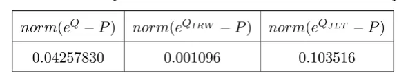
In a similar way,norm(eQ−P) = 0.04257830 is calculated by Matlab, when tol= 10−5. The error results are shown in the table below:
Table 4-2: Comparison of error values in the first example
norm(eQ−P) norm(eQIRW −P) norm(eQJ LT −P)
0.04257830 0.001096 0.103516
And we can also find that the calculation accuracy of the modified matrix, which we finally
get is one order of magnitude worse thanQIRW, but one order of magnitude better thanQJ LT.
5. Conclusions
Firstly, the logarithmic generated matrix to be optimized is obtained from the annual
transfer matrix of credit rating risk by the improved inverse scaling and squaring square
method.
Secondly, under the original K-S optimization model, the newly obtained logarithmic
ma-trix is modified to the Convex optimization problem of constraint of linear inequality by
dimensionality reduction, variable substitution and modification. The efficient set method is
used to optimize the Matlab calculation to satisfy the definition properties of the
generat-ing matrix. At the same time, the method has complete convergence and stability, and the
References:
[1] R.A.Jarrow,D.Lando and S.M.Turnbull, A Markov Model for the Term Structure of Credit Risk Spreads. Rev.Financial Stud, 1997, vol. 10(2), pp. 481-523.
[2] A.Kreinin and M.Sidelnikova, Regularization algorithm for transition matrices, Algo Re-search Quarterly, 2001, vol. 4, pp. 23-40.
[3] Ma Changfeng, Optimization method and its Matlab program design, Science Press, pp. 114-208(Chinese).
[4] Yuan Yaxiang and Sun Wenyu, Optimization Theory and Method, 1997, Beijing, Science Press(Chinese).
[5] R. B. Israel, J. S. Rosenthal and J. Z. Wei, Finding generators for Markov chains via empirical transition matrices,with applications to credit ratings, Math.Finance, 2001, vol. 11(2), pp. 245-265.
[6] Luo Yuanyuan, Genetic algorithm for solving linear inequality constrained optimization problems[Master dissertation], Graduate School of Science and Engineering, Nanjing Uni-versity of Aeronautics and Astronautics, 2007, vol. 11(Chinese).
[7] Masaaki Kijima, Monotonicities in a Markov Chain Model for Valuing Corporate Bonds Subject to Credit Risk, Mathematical Finance, 1998, vol. 8(3) , pp. 229-247.
[8] L. C. Thomas, D. E. Allen and E. Cowan, A hidden Markov chain model for the term structure of bond credit risk spreads, International Review of Financial Analysis, 2002, vol. 11(3), pp. 311-329.
[9] Aglaia Vasileiou and P.-C. G. Vassiliou, An inhomogeneous semi-Markov model for the term structure of credit disk spreads, .Advances in Applied Probability, 2006, vol. 38(1), pp. 171-198.
[10] Zeng Jian and Chen Junfang, The adjustment problem of transfer matrix in credit risk model, Journal of Systems Management, 2007, pp. 257-261(Chinese).
[11] T. R. Hurd and A. Kuznetsov, Affine Markov chain model of multifirm credit migration. Dept. of Mathematics and Statistics McMaster University, 2006, 12.
[12] Giuseppe Di Graziano and L. C. G. Gogers, A dynamic approach to the modeling of correlation credit derivatives using Markov chains, International Journal of Theoretical and Applied Finance. 2006, vol. 12(1).
[13] Wang Dingwei and Wang Junwei. Intelligent optimization method. Higher Education Press, First edition, 2007, 4(Chinese).
[14] Meng Xiuqing, Dynamic Evaluation of Corporate Credit Risk of Commercial Bank Com-panies [Master dissertation], Nanjing University of Science and Technology, 2013, 3(Chi-nese).
[15] Cetin B C, Barhen J and Burdick J W, Terminal repeller unconstrained subenergy tun-neling(TRUST) for fast global optimization, Optimization Theory and Applications, 1993, 77(1), pp. 97-126.
[17] Dr. Riddhi Garg, Symmetric Duality in Multi - Objective Programming. International Journal of Mathematics Trends and Technology, 2016, vol. 29(1), pp. 39-44.