The Thirty-Third AAAI Conference on Artificial Intelligence (AAAI-19)
MFBO-SSM: Multi-Fidelity Bayesian
Optimization for Fast Inference in State-Space Models
Mahdi Imani
Texas A&M UniversitySeyede Fatemeh Ghoreishi
Texas A&M University [email protected]Douglas Allaire
Texas A&M University [email protected]
Ulisses M. Braga-Neto
Texas A&M UniversityAbstract
Nonlinear state-space models are ubiquitous in model-ing real-world dynamical systems. Sequential Monte Carlo (SMC) techniques, also known as particle methods, are a well-known class of parameter estimation methods for this general class of state-space models. Existing SMC-based techniques rely on excessive sampling of the parameter space, which makes their computation intractable for large systems or tall data sets. Bayesian optimization techniques have been used for fast inference in state-space models with intractable likelihoods. These techniques aim to find the maximum of the likelihood function by sequential sampling of the parameter space through a single SMC approximator. Various SMC ap-proximators with different fidelities and computational costs are often available for sample-based likelihood approxima-tion. In this paper, we propose a multi-fidelity Bayesian op-timization algorithm for the inference of general nonlinear state-space models (MFBO-SSM), which enables simultane-ous sequential selection of parameters and approximators. The accuracy and speed of the algorithm are demonstrated by numerical experiments using synthetic gene expression data from a gene regulatory network model and real data from the VIX stock price index.
Introduction
Nonlinear state-space models are a popular class of time series models with numerous applications in fields such as statistics, economics, biology and more (Arnaud, Freitas, and Gordon 2001;Elliott, Aggoun, and Moore 2008; Capp´e, Moulines, and Ryden 2005). Sequential Monte Carlo (SMC) techniques, also known as particle methods (Arnaud, Fre-itas, and Gordon 2001; Kantas et al. 2015), are the most well-known class of techniques for estimation of param-eters of general nonlinear state space models from data. Several particle-based inference methodologies have been developed in recent years. The methods can be divided into two main categories: maximum-likelihood (ML) and Bayesian approaches. The techniques based on the ML per-spective either try to maximize the regular (“incomplete”) log-likelihood function (Johansen, Doucet, and Davy 2008) or the “complete” log-likelihood function; in the latter case,
Copyright c2019, Association for the Advancement of Artificial Intelligence (www.aaai.org). All rights reserved.
they are known as expectation maximization (EM) tech-niques (Sch¨on, Wills, and Ninness 2011; Wills et al. 2013). Bayesian techniques include particle marginal Metropolis-Hastings (PMMH) and particle-based Gibbs samplers (An-drieu, Doucet, and Holenstein 2010). All aforementioned methods rely on excessive sampling of the parameter space to avoid local optimum traps. However, for large systems and tall data sets, the cost of approximation of the inference function per parameter sample point can be computationally expensive, rendering intractable the computation of existing particle-based techniques.
Several techniques employ Bayesian optimization to cope with intractable likelihood functions, mostly in the con-text of approximate Bayesian computing (ABC) (Dahlin, Schon, and Villani 2015). The idea of these techniques is to construct a surrogate model representing the log-likelihood function over the parameter space, and efficiently search for its maximum through a single approximator (e.g., a parti-cle filter). The speed and accuracy of these methods are di-rectly impacted by the particle sample size used by the SMC approximator. Large particle sample sizes produce more ac-curate (high-fidelity) approximators at larger computational time/cost, while small particle sample sizes result in fast but less accurate (low-fidelity) approximators.
In this paper, we introduce the MFBO-SSM algorithm, a multi-fidelity Bayesian optimization method for the in-ference of general nonlinear state-space models. The pro-posed algorithm employs theknowledge gradient(KG) pol-icy (Frazier, Powell, and Dayanik 2008, 2009; Powell and Ryzhov 2012) for the simultaneous sequential selection of parameters and approximators, in such a way to achieve the largest single-period expected increase in the maximum of the inference function per unit cost.
The MFBO-SSM algorithm offers several benefits: • Fast and accurate inference due to the efficient
simultane-ous sequential selection of parameters and approximators; • Applicability to arbitrary point-based estimators, such as
ML and MAP techniques;
• Possibility of considering risk in the inference process; • Scalability to high-dimensional parameter spaces, due to
The accuracy and speed of the MFBO-SSM algorithm are demonstrated empirically by applying it to synthetic gene expression data from a gene regulatory network model and real data from the VIX stock price index.
Background
Nonlinear State-Space Models:
We assume the general nonlinear state-space model: xk = fk(xk−1,uk−1,nk, θ),
yk = gk(xk,vk, θ),
(1) for k = 1,2, . . . where xk ∈ X is the state variable,
uk ∈ Uis the input to the system, andyk ∈ Yis the
out-put of the system. The nonlinear functionsfk(.)andgk(.)
model the state and measurement dynamics, which are as-sumed to be partially-known with the unknown parameter vector θ ∈ Θ, whereΘ denotes the parameter space. Fi-nally,{nk,vk;k= 1,2. . . .}are mutually independent i.i.d.
processes, which are also independent ofx0. The parame-ter vectorθmodels uncertainty in both state and measure-ment processes. Equivalently,xk ∼ pθ(xk | xk−1,uk−1) andyk ∼pθ(yk | xk), wherepθ(.)is a probability density
or probability mass function. Without loss of generality and for the sake of simplicity, we will drop the inputuk−1 in what follows.
The inference problem consists of estimating the param-eter vectorθgiven the sequence of observed measurements y1:T = (y1, ...,yT). The maximum-likelihood (ML) and
the maximum a posteriori (MAP) estimators are given by: ˆ
θML = arg max
θ∈Θ logpθ(y1:T), ˆ
θMAP = arg max
θ∈Θ p(θ|y1:T) = arg max
θ∈Θ [logp(θ) + logpθ(y1:T)], (2)
wherep(θ)denotes the prior distribution of the parameter. Both ML and MAP estimators require the exact computation of the data log-likelihood function:
LT(θ) = logpθ(y1:T)
= logpθ(y1) + T
X
k=2
logpθ(yk|y1:k−1), (3)
where
pθ(yk |y1:k−1) =
Z
pθ(yk |xk)pθ(xk |y1:k−1)dxk,
(4) and
pθ(xk|y1:k−1) = Z
pθ(xk|xk−1)pθ(xk−1|y1:k−1)dxk−1.
(5) The integrals in (4) and (5) need to be replaced by summa-tions in the case of a discrete state space.
Sequential Monte Carlo: Auxiliary Particle Filter
The exact computation of (4) and (5) is not tractable in gen-eral and approximate methods, such as sequential Monte-Carlo (SMC), also known as particle filtering, must be used.SMC methods comprise a general class of techniques for inference of nonlinear state-space models (Arnaud, Freitas, and Gordon 2001; Kantas et al. 2015). The idea of these techniques is to approximate the target distribution using a finite sample drawn from a proposal distribution, using the fact that sampling from the proposal distribution is easier than from the target. The basic algorithm to perform particle filtering is calledsequential importance resampling(SIR). Here, we briefly review a variation of the SIR technique called the Auxiliary Particle Filter (APF) (Pitt and Shep-hard 1999).
The APF is an SMC method that efficiently predicts the location of particles with high probability at time stepk us-ing information up to time stepk−1via an auxiliary vari-ableζk. The method first draws a sample of points (particles)
from the joint distributionpθ(xk, ζk | y1:k), then drops the
auxiliary variable to obtain particles frompθ(xk |y1:k).
Let {˜xk−1,i, wk−1,i}Ni=1 be N particles and their asso-ciated weights at time k − 1 approximating pθ(xk−1 | y1:k−1). The process is divided into two stages. The first stage weights can be computed as:
vk,i = pθ(yk|µk,i)wk−1,i, (6)
fori= 1, . . . , N; whereµk,i is a characteristic ofxkgiven
˜
xk−1,i, which can be the mean, the mode or even a sample
from pθ(xk | x˜k−1,i)(Pitt and Shephard 1999). The
aux-iliary variables {ζk,i}Ni=1 are obtained by sampling from a discrete distribution:
{ζk,i}Ni=1∼Cat({˜vk,i}Ni=1), (7) where{v˜k,i}Ni=1 are the normalized first-stage weights, and Cat(a1, ..., aN) represents a categorical distribution with
probability mass functionf(ζ =i) = ai. Finally, the new
particles {x˜k,i}Ni=1 and associated second-stage weights {wk,i}Ni=1can be obtained as follows:
˜
xk,i ∼ pθ(xk |x˜k−1,ζk,i), wk,i =
pθ(yk |x˜k,i)
pθ(yk|µk,ζk,i)
. (8)
It is shown in (Pitt 2002) that:
pθ(yk |y1:k−1)≈ 1 N
N
X
i=1 vk,i
!
1 N
N
X
i=1 wk,i
!
, (9)
where the above quantity can be used for approximating the log-likelihood function in (3).
Related Work
Particle-Based Maximum-Likelihood (ML) Techniques: Existing particle-based ML techniques for inference of general nonlinear state-space models can be divided into three main categories:
point based on the approximated gradient at the current sample. The computational complexity of approximating the log-likelihood is of order O(N(T + 1)), where N is the number of particles and T is the length of the time series data. However, the unavoidable “resampling” step of particle filtering renders the approximated log-likelihood function discontinuous inθeven if the exact log-likelihood functionLT(θ)is continuous (Johansen, Doucet, and Davy
2008). Several importance-sampling methods have been introduced for approximation of the gradient function (De-Jong et al. 2012; Malik and Pitt 2011; Ionides, Bret´o, and King 2006). While some of these have computational com-plexity of orderO(N(T+ 1) logN), successful methods are O(N2(T + 1))(Kantas et al. 2015; Johansen, Doucet, and Davy 2008). In addition, these techniques require extensive sampling of the parameter space to avoid local optimum traps.
Expectation-Maximization Techniques: Unlike direct ML techniques, which attempt to maximize the “incomplete” log-likelihood functionLT(θ) = logpθ(y1:T),
expectation-maximization (EM) considers instead the “complete” log-likelihood function logpθ(x0:T,y1:T). The logic
be-hind this is that maximizing the complete log-likelihood is easier than the incomplete one. The EM algorithm thus consists of picking an initial guess θ = θ(0) and iterating two steps: 1) E-Step: Compute Q(θ, θ(n)), 2) M-Step: Find θ(n+1) = argmax
θ∈ΘQ(θ, θ(n)), where Q(θ, θ(n)) = E
x0:T
logpθ(x0:T,y1:T)|y1:T, θ(n)
. These steps need to be performed iteratively until a stopping criterion is met. Exact computation of the E-step is not possible for general nonlinear state-space models and one needs to use particle methods for its approximation. Two popular particle smoothers are the backward simula-tion smoother (Godsill, Doucet, and West 2004) and the reweighting particle smoother (H¨urzeler and K¨unsch 1998), which have lead to two different particle-based EM algo-rithms for general nonlinear state-space models introduced in (Sch¨on, Wills, and Ninness 2011) and (Wills et al. 2013) respectively. The computational complexity of both methods are of order O(N2(T + 1)). It should also be noted that the closed-form solution for the M-step might not be achievable in general, posing another expensive computation. Similar to direct ML techniques, this class of estimators requires several iterations to avoid local optimum traps.
Particle-Based Bayesian Techniques: There are several particle-based Bayesian techniques for the inference of general nonlinear state-space models. An important rep-resentative is the particle marginal Metropolis-Hastings (PMMH) method (Andrieu, Doucet, and Holenstein 2010). Given that θ is the current sample and pθ(y1:T) is the
approximated likelihood by a particle filter (e.g., APF) associated withθ, one needs to draw a new sample param-eterθ0 ∼ q(θ0 | θ)from the proposal distribution and run a particle filter to approximate the likelihood pθ0(y1:T).
Then, the new parameterθ0 gets accepted with probability min{1, pθ0(y1:k)p(θ0)q(θ|θ0)/pθ(y1:k)p(θ)q(θ0|θ)}.
This process continues for a large enough (usually pre-specified) number of iterations in order to ensure good inference performance.
All the aforementioned techniques in the first two cate-gories require extensive sampling of the parameter space to approximate the complete/incomplete log-likelihood func-tion. For large systems, which require a large number of particles, and for tall data sets, the computational cost of ap-proximating the log-likelihood function per parameter sam-ple point can be prohibitive.
Surrogate-Based Techniques: This class of techniques has been developed for fast inference in SSMs with in-tractable likelihood functions (Dahlin, Schon, and Vil-lani 2015; Dahlin and Lindsten 2013). The idea of these methods is to use Gaussian process regression for log-likelihood approximation, and apply Bayesian optimization techniques for efficient exploration of the maximum of the log-likelihood function using a single SMC approximator (i.e., a particle filter with a fixed particle sample size). The computational complexity of these techniques is of order O(N(T+ 1))for each function evaluation. Despite the suc-cess of these techniques, their accuracy and speed are highly impacted by the choice of particle sample size. Large par-ticle sample sizeN makes the inference process very slow, while improving accuracy. On the other hand, small particle sample size reduces accuracy, while accelerating the speed of the inference process. The main focus of the current pa-per is an efficient strategy for simultaneous parameter and approximator selection at each iteration of the learning pro-cess to achieve fast and accurate inference.
Proposed Algorithm
Modeling the Inference Function by a Gaussian
Process:
We account for the correlation in the inference function by employing Gaussian process regression (Rasmussen and Williams 2006). Let z(θ)be the inference function at pa-rameterθ∈Θapproximated by a particle filter withN par-ticles associated with parameter θ (e.g., z(θ)refers to the approximate log-likelihood and log-a posteriori probability for ML and MAP techniques respectively). Note thatz(θ) is a stochastic process, due to the uncertainty arising by the use of a particle filter.
The following model is considered here for the inference function:
z(θ) ≈ h(θ) + ∆hN, (10)
where h(θ) is a Gaussian process (GP) over the parame-ter space Θ, and ∆hN is a zero-mean Gaussian residual
with variance σN2, which models, for all parameters, the uncertainty arising from the use of a particle filter with N particles. Large particle sample sizes N correspond to smallerσ2
N.
correla-tion betweenθandθ0. A common kernel choice for a contin-uous parameter space is the well-known exponential kernel function (Rasmussen and Williams 2006).
Letθm = (θ(1), . . . , θ(m))be a sample from the
param-eter space, with the approximated inference function com-puted by running m particle filters with particle sample sizesnm= (N1, ..., Nm), and evaluated objective function
zm= [z(θ(1)), . . . , z(θ(m))]T. The posterior distribution of
h(θ)in equation (11) can be obtained as (Rasmussen and Williams 2006):
h(θ)|θm,nm,zm∼ N ¯hm(θ),covm(θ, θ), (12)
where
¯
hm(θ) =µ(θ) +Kθ,θm(Kθm,θm+Σnm)
−1
(zm−µ(θm)),
covm(θ, θ) = k(θ, θ)−Kθ,θm(Kθm,θm+Σnm)
−1
KTθ,θm,
(13) Σnm is a diagonal matrix of sizemwithith diagonal
ele-ment(Σnm)ii=σ
2
Ni, and
Kθ,θ0 =
k(θ1, θ10) . . . k(θ1, θ0n)
..
. . .. ... k(θl, θ10) . . . k(θl, θ0n)
, (14)
forθ ={θ1, ..., θl},θ0 ={θ01, ..., θ0n}.Using the above
for-mulation, the inference function before observing any data is modeled by a zero-mean Gaussian process with covari-ancek(θ, θ), while at iterationm, the inference function is predicted based on the sequence of queried samplesθm, the
approximate inference function valueszm, and the particle
sample sizesnmused for these approximations. The
uncer-tainty in the inference function, which is modeled by the co-variance function in equation (12), decreases as more points are sampled from the parameter space and added to the GP.
The hyperparameters of the Gaussian process, such as the parameters of the kernel function or the mean function, can be estimated at each time point using the marginal likelihood function (Rasmussen and Williams 2006):
zm|θm,nm∼ N(µ(θm),Kθm,θm+Σnm). (15)
Notice that, due to the difficulty of choosing a proper model for the mean function and its impact on the inference accu-racy, a possible option is to useµ(θ) = mini=1,...,mzm(i).
This adaptive constant mean avoids the challenging task of picking a proper parametric model for the mean function, and also prevents over-estimation of the objective function over regions that have not been explored well.
Simultaneous Sequential Selection of Parameter
and Particle Sample Size:
To boost the speed of the inference process and overcome the computational intractability of existing techniques, we introduce a multi-fidelity Bayesian optimization algorithm for the inference of general nonlinear state-space models (MFBO-SSM).
Letσ2
N be the variance of the objective function
approx-imated by a particle filter with N particles. The value of the noise statisticsσ2
N mainly depends on the particle
sam-ple sizeNfor the log-likelihood approximation. This value
can be quantified in three possible ways: 1) running mul-tiple particle filters with a fixed particle sample size at an arbitrary sample of the parameter space and computing the sample variance of the approximated log-likelihood values; 2) using available theoretical upper bounds on the approxi-mation error of a particle filter with a fixed particle sample size (Whiteley 2013; Olsson and Ryden 2008); 3) treating the noise parameters as hyperparameters and learning them on the fly according to the marginal likelihood in (15).
The variance issue is linked to the computational com-plexity cN of particle filtering algorithms, which increases
linearly with the number of particles. Thus, largeN corre-sponds to an approximator with smaller variance (high- fi-delity) and high computational complexity, whereas smallN models an approximator with large uncertainty (low-fidelity) but low computational complexity.
To better understand the intuition behind the proposed al-gorithm, let us consider a simple nonlinear continuous state-space model (Doucet, Godsill, and Andrieu 2000; Godsill, Doucet, and West 2004):
xk+1 = 0.5xk+θ
xk
1 +x2
k
+ 8 cos(1.2k) +nk,
yk = 0.05x2k+vk,
(16)
wherenk ∼ N(0,0.001), vk ∼ N(0,0.01), andθ is the
only parameter of the system, with true valueθ∗ = 25. For a time series of length100, the exact log-likelihood is plot-ted in black in Figure 1. The Gaussian process approximaplot-ted by10sample points from the parameter space with particle sample size N1 = 20is plotted in Figure 1(a). This low-fidelity approximator has varianceσN1 = 10,000. It can be
seen that 10sample points from the parameter space have properly captured the log-likelihood function with this ap-proximator. Figure 1(b) displays the constructed GP with N2= 100and two sample points from the parameter space. For this high-fidelity approximator,σN2 = 500. These two
approximations have the same computational complexity, sincecN1/cN2 = N1/N2 = 20/100. However, the mean
of the GP corresponding to the high-fidelity approximator is far from the exact log-likelihood function.
0 10 20 30 40 50
-10 -5 0 5
104
95% Confidence Interval
0 10 20 30 40 50
-10 -5 0 5
104
95% Confidence Interval
to select simultaneously good sample points in the parame-ter space and good approximators of the log-likelihood func-tion during the learning process. Finding an optimal (finite or infinite horizon) strategy is a challenging task. In the next paragraphs, we describe how a Bayesian optimization framework, in particular the knowledge gradient policy (Fra-zier, Powell, and Dayanik 2008, 2009), can be employed for tackling this problem.
Letθm = (θ(1), ..., θ(m))be a sample from the
param-eter space with associated approximated inference function valueszm = [z(θ(1)), ..., z(θ(m))]T computed by particle
filters with particle sample sizesnm = (N1, ..., Nm). By
constructing a GP given all available information up to iter-ationm, a given sample pointθ∈Θhas expected inference functionh¯m(θ) =E[h(θ)|θm,nm,zm], according to (13),
and
ˆ
θ∗GP = argmax
θ∈Θ ¯
hm(θ). (17)
If an additional pair of parameter and approximator is to be selected from the parameter space and set of approximators, we would like to choose the pair with the highest single-period expected increase in the maximum of the inference function per unit cost. This policy, which is referred to as a multi-fidelity knowledge gradient policy, can be formulated as:
(θ(m+1), Nm+1) = argmax
(θ,N)∈(Θ,N) 1 cN
Em
max
θ0∈ΘE
h
h(θ0)|θm,nm,zm, θ(m+1)=θ, Nm+1=N
i
−max
θ0∈ΘE
h(θ0)|θm,nm,zm
,
(18) whereNdenotes a finite set of particle sample sizes corre-sponding to a finite number of approximators, andEm
de-notes expectation over the unobserved inference function at pointθ(m+1)approximated by a particle filter (approxima-tor) withNm+1particles, given all available information up to iterationm.
Exact computation of (18) is not possible over an infinite parameter space. However, given a finite set of alternatives
A⊂Θ, we can write the approximation:
(θ(m+1), Nm+1) = argmax (θ,N)∈(A,N)
1 cN
EI (θ, N), (19)
where
EI (θ, N) =
Em
max
θ0∈ AE
h
h(θ0)|θm,nm,zm, θ(m+1)=θ, Nm+1=N
i
−max
θ0∈AE
h(θ0)|θm,nm,zm
,
(20) for θ ∈ A and N ∈ N. The knowledge gradient
al-gorithm (Frazier, Powell, and Dayanik 2008, 2009) pro-vides a closed-form solution for computation of the ex-pected increase EI (θ, N) in the maximum of the objec-tive function in (20). The feature of the knowledge gradient policy to account for the uncertainty in the log-likelihood
function approximation is a reason of choosing this ac-quisition function over other Bayesian optimization tech-niques, such as expected improvement (Jones 2001) and en-tropy search (Hern´andez-Lobato, Hoffman, and Ghahramani 2014).
The finite set of alternatives A ⊂ Θshould be selected
based on the goal of the inference process. In particular, the set of alternatives for ML estimation can be obtained us-ing hypercube samplus-ing (McKay, Beckman, and Conover 1979), whereas for MAP estimation, the alternative set could be provided by a sample drawn from the prior distribution. The set of particle sample sizes (number of approximators) needs to be chosen based on the size of the system and the amount of data. However, the algorithm is fairly robust against this choice: in our numerical experiments, we ob-served that “small”, “medium” and “large” particle sample sizes all lead to good inference accuracy and speed.
After selection of θ(m+1) andN
m+1 using (19), a par-ticle filter with Nm+1 particles associated with parameter θ(m+1) is run and the Gaussian process is updated based on θm+1 = (θm, θ(m+1)), nm+1 = (nm, Nm+1), and zm+1 = [zm, z(θ(m+1))]T. This procedure continues until a
stopping criterion is met, which might be a threshold for the change in the maximum of the mean of the constructed GP in consecutive iterations, or a pre-specified limit on the num-ber of iterations. It should be noted that the complexity of the MFBO-SSM algorithm at iterationmis approximately O(max{Nm+1(T + 1), m3}), whereNm+1is the number of particles used for the objective function approximation, andTis the length of the time series data.
The Gaussian processes constructed over the log-likelihood function for the system in (16) at different iter-ations of the proposed algorithm are plotted in Figure 2. It can be seen that all9initial sample parameters prescribed by MFBO-SSM are from the low-fidelity approximator (N1= 20), but the last three sample parameters are evaluated by the high fidelity approximator (N2= 100). Indeed, the low-fidelity approximator with5times less computational com-plexity has been initially used for proper exploration of the parameter space. Then, as the expected increase in the max-imum of the inference function per unit cost using the use of first approximator becomes small, the high-fidelity approx-imator is performed for proper exploitation. As we will see in the next section, this key feature of the MFBO-SSM al-gorithm results in an inference process that is both fast and accurate, as compared to the existing techniques.
Experiments
All experiments have been conducted on a PC with an Intel Core i7-4790 [email protected] clock and 16 GB of RAM.
0 10 20 30 40 50 -10
-5 0 5
104
95% Confidence Interval
0 10 20 30 40 50
-10 -5 0 5
104
95% Confidence Interval
0 10 20 30 40 50 -10
-5 0 5
104
95% Confidence Interval
Figure 2: Constructed GP and estimated parameter at different iterations of MFBO-SSM for the system in (16).
1 10 20 30
Running Time (mins)
0 0.1 0.2 0.3
Average MSE
1 10 20 30
Running Time (mins) 0
0.1 0.2 0.3 0.4 0.5 0.6
1 10 20 30
Running Time (mins) 0
5 10 15 20
1 10 20 30
Running Time (mins)
0 2 4 6
Figure 3: Average MSE against running time in minutes for different inference algorithms using synthetic data from the stochas-tic volatility model.
Algorithm 1MFBO-SSM Algorithm
1: Set the alternative setA, and the particle setN, the costcN and varianceσ2
Nof the particle filter withN∈Nparticles. 2: Construct a GP over parameterθ.
3: m=−1,θ0={},n0={},z0={}. Whilestopping criterion is not met
4: m=m+ 1.
5: (θ(m+1), N
m+1) = argmax(θ,N)∈(A,N) 1
cNEI (θ, N)where
EI (θ, N)is defined in Eq. (20).
6: Run a particle filter tuned toθ(m+1)with particle sizeNm+1 to getz(θ(m+1)).
7: θm+1 = {θm, θ(m+1)},nm+1 = {nm, Nm+1},zm+1 = {zm, z(θ(m+1))}.
8: Update GP according to (θm+1,nm+1,zm+1). End While
9: θˆ∗GP = argmaxθ∈Θh¯m(θ), whereh¯m(θ)is the mean of the
final GP.
this model are:
xk = φxk−1+ (1−φ)µ+σnk, nk∼ N(0,1)
yk = βexp(xk/2)vk, vk∼ N(0,1).
(21)
The performance of the MFBO-SSM algorithm is as-sessed using both synthetic and real data. For synthetic data, 100time series of length4000are drawn from the model in (21) with initial statex0∼ N(0, σ2/1−φ2). While there is only a single state variable, the time-varying process neces-sitates the use of a large number of particles. MFBO-SSM
1 1008 2014 3266
Running Time (mins) 0
20 40 60 80
VIX Index
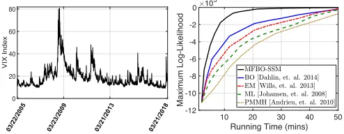
10 20 30 40 50 Running Time (mins) -12
-10 -8 -6 -4 -2 0
Maximum Log-Likelihood
105
Figure 4: Daily return data for the VIX stock price index and average maximum log-likelihood against running time in minutes for different inference algorithms using these data.
Table 1: Results for the cell-cycle gene regulatory network.
Average MSE (running time per minutes)
N BO (Dahlin, Schon, and Villani 2015) EM (Wills et al. 2013) ML (Johansen, Doucet, and Davy 2008) PMMH (Andrieu, Doucet, and Holenstein. 2010) MFBO-SSM
20,000 9.412 (88.15) 9.473 (166.98) 10.238 (199.39) 10.991 (354.45)
6.904 (35.59)
40,000 6.902 (189.24) 6.862 (341.92) 7.827 (418.09) 7.618 (722.90)
Figure 5: Average number of particles used by the MFBO-SSM algorithm against iteration number for the daily return data for the VIX stock price index.
Figure 3 displays the average MSE of estimation of the dif-ferent parameters against running time in minutes. One can observe that the accuracy at the same speed achieved by MFBO-SSM is significantly higher than for the other meth-ods.
Real data with length3273from the VIX stock price in-dex recorded between March 2005 and March 2018 have also been used in our analysis. The data are displayed in the left panel of Figure 4. The average maximum of the log-likelihood function against running time is displayed in the right panel of Figure 4. One can observe that the log-likelihood is maximized faster by the MFBO-SSM algo-rithm than by the other methods. The average number of particles used by the MFBO-SSM algorithm against itera-tion number is displayed in Figure 5. It can be seen that the MFBO-SSM algorithm picks the low-fidelity approximator (i.e., the particle filter with N1 = 100) most of the time at early iterations, for cheap exploration, while selecting the two other expensive approximators with particle sample sizesN2= 1000andN3= 5000only at later iterations, for better exploitation.
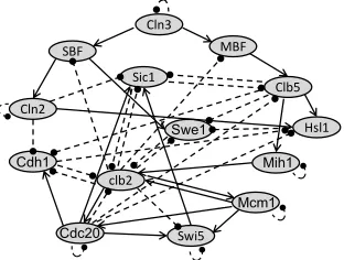
Cell-Cycle Gene Regulatory Network Example:In the second experiment, we consider the cell cycle gene regu-latory network model in (Radmaneshfar and Thiel 2012). This is a Boolean network consisting of 14 genes, where each gene can be activated or inactivated. Hence, there are 214 = 16384different possible system states. The pathway diagram for this gene regulatory network is displayed in Fig-ure 6. Normal arrows represent activating regulations and dash arrows represent suppressive regulations. With vector xkcontaining the expression state of all 14 genes at timek,
the Boolean state process can be written as:
xk = Axk−1⊕nk, (22)
wherevmaps the positive elements of vectorvto1and oth-ers to0,nkis the process noise, andA= [aij]is the
connec-tivity matrix. Parameteraij specifies the type of regulation
from genej to gene i: it is equal to+1for the activating regulation, −1 for the inactivating regulation and 0for no regulation. The process noisenk is assumed to have
inde-pendent components distributed as Bernoulli(p), where the noise parameterpgives the amount of “perturbation” to the Boolean state process. In our simulation, we setp= 0.01.
Cln3
MBF
Clb5
Hsl1
Swi5 Sic1 SBF
Cln2
clb2
Mcm1
Cdc20
Swe1
Cdh1 Mih1
Figure 6: Pathway diagram for the cell-cycle gene regulatory network model.
We assume a Gaussian linear observation model:
yk = µ+Dxk+vk, k= 1,2, . . . (23)
wherevk∼ N(0, σ2I)is an uncorrelated zero-mean
Gaus-sian noise vector,µis a vector of baseline gene expressions (corresponding to the “zero” state for each gene) andDis a diagonal matrix containing differential expression values for each gene along the diagonal (these indicate by how much the activated state of each gene is over-expressed over the in-activated state). Such a Gaussian linear model is an appropri-ate model for many important gene-expression measurement technologies, such as cDNA microarrays (Chen, Dougherty, and Bittner 1997 )and live cell imaging-based assays (Hua et al. 2012). Here, we assume that µ = [µ, . . . , µ]T and
In Table 1, we can observe that for both particle sample sizes, the MFBO-SSM algorithm achieves good accuracy with a much smaller running time than the other algorithms. Indeed, MFBO-SSM is2.5times faster than the fastest com-petitor forN = 20,000and5times faster forN = 40,000. These results demonstrate the ability of MFBO-SSM in speeding up inference for both large systems and tall data sets, at similar or better accuracy levels.
Conclusion
In this paper, we introduced the MFBO-SSM algorithm for fast and accurate inference of parameters of nonlinear state-space models. The proposed algorithm can handle large sys-tem sizes and tall data sets. MFBO-SSM alleviates the com-putational expense associated with sample-based approxi-mations of the inference function by constructing a Gaus-sian process for modeling the correlation in the inference function, and learns the maximum of this surrogate model by simultaneous selection of sample parameters and parti-cle sample sizes for its SMC approximation. In numerical experiments using real and synthetic data, the proposed al-gorithm performed significantly faster than competing algo-rithms, at similar or better accuracy levels.
References
Andrieu, C.; Doucet, A.; and Holenstein, R. 2010. Particle Markov chain Monte Carlo methods.Journal of the Royal Statistical Soci-ety: Series B (Statistical Methodology)72(3):269–342.
Arnaud, D.; Freitas, N.; and Gordon, N. 2001. Sequential Monte Carlo methods in practice. New York: Springer Science+ Business Media, Inc. LLC.
Capp´e, O.; Moulines, E.; and Ryden, T. 2005.Inference in Hidden Markov Models. Springer.
Chen, Y.; Dougherty, E. R.; and Bittner, M. L. 1997. Ratio-based decisions and the quantitative analysis of cDNA microarray im-ages.Journal of Biomedical optics2(4):364–374.
Chib, S.; Nardari, F.; and Shephard, N. 2002. Markov chain Monte Carlo methods for stochastic volatility models. Journal of Econo-metrics108(2):281–316.
Dahlin, J., and Lindsten, F. 2013. Particle filter-based Gaus-sian process optimisation for parameter inference. arXiv preprint arXiv:1311.0689.
Dahlin, J.; Schon, T. B.; and Villani, M. 2015. Bayesian opti-misation for fast approximate inference in state-space models with intractable likelihoods.arXiv preprint arXiv:1506.06975.
DeJong, D. N.; Liesenfeld, R.; Moura, G. V.; Richard, J. F.; and Dharmarajan, H. 2012. Efficient likelihood evaluation of state-space representations.Review of Economic Studies80(2):538–567. Doucet, A.; Godsill, S.; and Andrieu, C. 2000. On sequential Monte Carlo sampling methods for Bayesian filtering. Statistics and computing10(3):197–208.
Elliott, R. J.; Aggoun, L.; and Moore, J. B. 2008.Hidden Markov models: estimation and control, volume 29. Springer Science & Business Media.
Frazier, P. I.; Powell, W. B.; and Dayanik, S. 2008. A knowledge-gradient policy for sequential information collection. SIAM Jour-nal on Control and Optimization47(5):2410–2439.
Frazier, P.; Powell, W.; and Dayanik, S. 2009. The knowledge-gradient policy for correlated normal beliefs. INFORMS journal on Computing21(4):599–613.
Godsill, S. J.; Doucet, A.; and West, M. 2004. Monte Carlo smoothing for nonlinear time series. Journal of the american sta-tistical association99(465):156–168.
Hern´andez-Lobato, J. M.; Hoffman, M. W.; and Ghahramani, Z. 2014. Predictive entropy search for efficient global optimization of black-box functions. InAdvances in neural information processing systems, 918–926.
Hua, J.; Sima, C.; Cypert, M.; Gooden, G. C.; Shack, S.; Alla, L.; Smith, E. A.; Trent, J. M.; Dougherty, E. R.; and Bittner, M. L. 2012. Dynamical analysis of drug efficacy and mechanism of action using GFP reporters. Journal of Biological Systems
20(04):403–422.
H¨urzeler, M., and K¨unsch, H. R. 1998. Monte Carlo approxima-tions for general state-space models.Journal of Computational and Graphical Statistics7(2):175–193.
Ionides, E. L.; Bret´o, C.; and King, A. A. 2006. Inference for non-linear dynamical systems.Proceedings of the National Academy of Sciences103(49):18438–18443.
Johansen, A. M.; Doucet, A.; and Davy, M. 2008. Particle meth-ods for maximum likelihood estimation in latent variable models.
Statistics and Computing18(1):47–57.
Jones, D. R. 2001. A taxonomy of global optimization meth-ods based on response surfaces. Journal of global optimization
21(4):345–383.
Kantas, N.; Doucet, A.; Sing, S. S.; Maciejowski, J.; and Chopin, N. 2015. On particle methods for parameter estimation in state-space models. Statistical science30(3):328–351.
Malik, S., and Pitt, M. K. 2011. Particle filters for continuous likelihood evaluation and maximisation. Journal of Econometrics
165(2):190–209.
McKay, M. D.; Beckman, R. J.; and Conover, W. J. 1979. Com-parison of three methods for selecting values of input variables in the analysis of output from a computer code. Technometrics
21(2):239–245.
Olsson, J., and Ryden, T. 2008. Asymptotic properties of particle filter-based maximum likelihood estimators for state space models.
Stochastic Processes and their Applications118(4):649–680. Pitt, M. K., and Shephard, N. 1999. Filtering via simulation: Auxil-iary particle filters.Journal of the American statistical association
94(446):590–599.
Pitt, M. K. 2002. Smooth particle filters for likelihood evaluation and maximisation. University of Warwick, Department of Eco-nomics.
Powell, W. B., and Ryzhov, I. O. 2012. Optimal learning, volume 841. John Wiley & Sons.
Radmaneshfar, E., and Thiel, M. 2012. Recovery from stress–a cell cycle perspective. Journal of computational interdisciplinary sciences3(1-2):33.
Rasmussen, C. E., and Williams, C. K. I. 2006.Gaussian processes for machine learning. MIT Press.
Sch¨on, T. B.; Wills, A.; and Ninness, B. 2011. System identifica-tion of nonlinear state-space models.Automatica47(1):39–49. Whiteley, N. 2013. Stability properties of some particle filters.The Annals of Applied Probability23(6):2500–2537.