The Thirty-Third AAAI Conference on Artificial Intelligence (AAAI-19)
IPOMDP-Net: A Deep Neural Network for Partially
Observable Multi-Agent Planning Using Interactive POMDPs
Yanlin Han, Piotr Gmytrasiewicz
Department of Computer ScienceUniversity of Illinois at Chicago Chicago, IL 60607
Abstract
This paper introduces the IPOMDP-net, a neural network architecture for multi-agent planning under partial observ-ability. It embeds an interactive partially observable Markov decision process (I-POMDP) model and a QMDP planning algorithm that solves the model in a neural network archi-tecture. The IPOMDP-net is fully differentiable and allows for end-to-end training. In the learning phase, we train an IPOMDP-net on various fixed and randomly generated en-vironments in a reinforcement learning setting, assuming ob-servable reinforcements and unknown (randomly initialized) model functions. In the planning phase, we test the trained network on new, unseen variants of the environments under the planning setting, using the trained model to plan without reinforcements. Empirical results show that our model-based IPOMDP-net outperforms the other state-of-the-art model-free network and generalizes better to larger, unseen environ-ments. Our approach provides a general neural computing ar-chitecture for multi-agent planning using I-POMDPs. It sug-gests that, in a multi-agent setting, having a model of other agents benefits our decision-making, resulting in a policy of higher quality and better generalizability.
Introduction
Decision-making under partial observability is fundamen-tally important but computationally hard, especially in multi-agent settings. In partially observable multi-agent en-vironments, an agent needs to deal with uncertainties from its own models as well as impacts from other agents ac-tions caused by their models. To learn policies in such settings, one approach is to learn models and solve them through planning. If the models are known, it reduces to a planning problem and can be formulated as an interactive partially observable Markov decision process (I-POMDP) (Gmytrasiewicz and Doshi 2005). Although approximate al-gorithms have made progress on mitigating the computing complexity (Doshi and Gmytrasiewicz 2009; Han and Gmy-trasiewicz 2018), solving I-POMDPs exactly is still com-putationally intractable for the worst case. Moreover, con-structing I-POMDP models manually or learning them from observations remains difficult. An alternative approach is to learn policies directly, such as using model-free
reinforce-Copyright c2019, Association for the Advancement of Artificial Intelligence (www.aaai.org). All rights reserved.
ment learning methods, in which the rewards are usually as-sumed obtainable. While the model-free policy learning can be end-to-end, it lacks the model information for effective generalization (Karkus, Hsu, and Lee 2017). Particularly, in the multi-agent domain, other agents’ actions impact the en-vironment, which indirectly impact our policies. Therefore, we prefer a model-based approach, since having a model of other agents helps our reasoning about their actions and con-sequently benefits our decision making.
The unprecedented success of deep neural networks (DNNs) in supervised learning (Ciregan, Meier, and Schmidhuber ; Farabet et al. 2013; Krizhevsky, Sutskever, and Hinton 2012) provides new approaches to decision making under uncertainty. Convolutional neural networks (CNNs) and recurrent neural networks (RNNs) have been applied to tasks like Atari games (Mnih et al. 2015), robotics (Levine et al. 2016), and 2D path planning (Karkus, Hsu, and Lee 2017). In these tasks, a DNN is trained to approximate a policy function that maps an agent’s observations to opti-mal actions. The deep Q-network (DQN), which consists of convolutional layers for feature extraction and a fully con-nected layer for mapping features to actions, tackles many Atari games with the same network architecture (Mnih et al. 2015). DQN is inherently reactive and lacks explicit plan-ning computation (Tamar et al. 2016). The deep recurrent Q-network (DRQN) extends DQN to the partially observ-able domain by replacing the fully connected layer with a recurrent long short-term memory (LSTM) (Hochreiter and Schmidhuber 1997) layer to integrate temporal information (Hausknecht and Stone 2015). Furthermore, the value iter-ation network (VIN) started to embed specific computiter-ation structures (Tamar et al. 2016), particularly the value iteration algorithm, in the network architecture and solves fully ob-servable Markov decision processes (MDPs). The QMDP-net further embeds a POMDP model and a QMDP planning algorithm that solves the model in a RNN (Karkus, Hsu, and Lee 2017). However, all the discussed neural networks are either model-free or for single-agent settings. Unless we model other agents’ impact as noise and embed it into the world dynamic, which often leads to inferior solution qual-ity, it is not feasible to directly apply these networks into a multi-agent partially observable domain.
par-tial observability. We extends the QMDP-net to a multi-agent domain by combining an interactive POMDP (I-POMDP)(Gmytrasiewicz and Doshi 2005) model with a QMDP planning algorithm and embedding both in a re-current neural network. We implement the IPOMDP-net on GPU-based computing devices and train it on problems of various sizes and dimensions. The training starts from ran-domly initialized weights, and is performed in a reinforce-ment learning fashion assuming the reward is obtainable. We then evaluate the trained IPOMDP-net by comparing its performance with another state-of-the-art model-free neural network. During the testing, we remove the obtainable re-ward assumption of all trained neural networks and test them on new unseen settings of the same problems. Therefore, they are using learned policies and acting based on observa-tion and acobserva-tion sequences in the same way as the symbolic I-POMDP does. We show empirical results that our based IPOMDP-net outperforms the state-of-the-art model-free network in different tasks.
Our approach provides a general neural computing ar-chitecture for multi-agent planning using I-POMDPs. It combines the benefits of free learning and model-based planning. Compared with model-free networks, the IPOMDP-net trained on small problem sizes generalizes more effectively to larger difficult settings. It suggests that, in a multi-agent setting, having a model of other agents ben-efits our decision-making, resulting in a policy of higher quality and better generalizability.
Background
In this section, we will briefly introduce the underlying multi-agent planning model, the interactive POMDP (Gmy-trasiewicz and Doshi 2005), that is encoded in our neural network architecture.
I-POMDP Framework
I-POMDPs generalize POMDPs (Kaelbling, Littman, and Cassandra 1998) to multi-agent settings by including mod-els of other agents in the belief state space (Gmytrasiewicz and Doshi 2005). The resulting hierarchical belief structure represents an agent’s belief about the physical state, belief about the other agents and their beliefs about others’ be-liefs, and can be nested infinitely in this recursive manner. For simplicity, we consider two interacting agentsiandj. This formalism generalizes to more number of agents in a straightforward manner.
A computable finitely nested interactive POMDP of agent i, I-POMDPi,l, is defined as:
I-P OM DPi,l=hISi,l, A,Ωi, Ti, Oi, Rii (1)
whereISi,lis a set of interactive states, defined asISi,l = S×Mj,l−1, l ≥ 1,S is the set of physical states,Mj,l−1
is the set of possible models of agentj, andlis the strategy (nesting) level.
In this paper, we focus on a specific subset of model classes, the intentional models, which ascribe beliefs, preferences, and rationality in action selection to other agents. Theintentionalmodels, usually denoted asΘj,l−1,
of agent j at level l − 1 is defined as θj,l−1 =
hbj,l−1, A,Ωj, Tj, Oj, Rj, OCji, where bj,l−1 is agent j’s
belief nested to the level (l −1), bj,l−1 ∈ ∆(ISj,l−1),
andOCj isj’s optimality criterion. It can be rewritten as θj,l−1 =hbj,l−1,θˆji, whereθˆj includes all elements of the intentional model other than the belief.
TheISi,lcan be defined in an inductive manner:
ISi,0=S, θj,0={hbj,0,θˆji:bj,0∈∆(S)}
ISi,1=S×θj,0, θj,1={hbj,1,θˆji:bj,1∈∆(ISj,1)}
... (2)
ISi,l=S×θj,l−1, θj,l={hbj,l,θˆji:bj,l∈∆(ISj,l)}
All remaining components in an I-POMDP are similar to those in a POMDP.A =Ai×Ajis the set of joint actions of all agents.Ωiis the set of agent i’s possible observations. Ti:S×A×S→[0,1]is the transition function.Oi:S× A×Ωi→[0,1]is the observation function.Ri:ISi×A→
Ris the reward function.
Interactive Belief Update
Given the definitions above, the interactive belief update can be performed as follows, by considering others’ actions and anticipated observations:
bti,l(ist) =P r(ist|b t−1 i,l , a
t−1 i , o
t
i) (3)
=α X
ist−1
bi,l(ist−1) X
atj−1
P r(atj−1|θj,lt−−11)T(st−1, at−1, st)×
Oi(st, at−1, oti) X
ot j
Oj(st, at−1, otj)τ(bt −1 j,l−1, a
t−1 j , o
t j, bt,l−1)
Conveniently, the equation above can be summarized as bti,l=SE(bi,lt−1, ati−1, oti).
Compared with POMDP, there are two major differences. First, the probability of other’s actions given his models needs to be computed since the state now depends on both agents’ actions (the second summation). Second, the model-ing agent needs to update his beliefs based on the anticipa-tion of what observaanticipa-tions the other agent might get and how it updates (the third summation).
While exact interactive belief update is intractable, there are sampling-based approximations using customized inter-active version of particle filters (Doshi and Gmytrasiewicz 2009;?), which will be embedded in the IPOMDP-net in a neural analogy.
The value iteration for I-POMDP is performed on interac-tive belief states in the following way:
V(θi,l) = max ai∈Ai
Q(θi,l, ai) (4)
= max
ai∈Ai
n X
is∈IS
bi,l(is)ERi(is, ai)+
γ X oi∈Ωi
P(oi|ai, bi,l)V(hSE(bi,l, ai, oi),θˆii)
o
Then the optimal action,a∗i, for an infinite horizon crite-rion with discounting, is part of the set of optimal actions, OP T(θi), for the belief state:
OP T(θi,l) = arg max ai∈Ai
Q(θi,l, ai) (5)
IPOMDP-Net
Overview
The IPOMDP-net is a neural analogy of the I-POMDP framework. As a recurrent neural network, it approximates the belief update as well as the policy function that maps the belief states to optimal actions. Similarly to the QMDP-net (Karkus, Hsu, and Lee 2017), it combines a parameterized model with an approximate algorithm that solves the model in a single, differentiable neural network. But we extend it to the multi-agent setting by embedding the I-POMDP model and the QMDP algorithm into the network architecture. This extension is non-trivial, as will be shown in the following section, because embedding an I-POMDP in the network re-quires encoding the sampling-based belief update algorithm and using sub-network modules to represent the hierarchical interactive belief structure.
Formally, letI−P OM DPi,l(w) = hISi,l(·|w), A,Ωi, Ti(·|w), Oi(·|w), Ri(·|w)i be the embedded I-POMDP model, where each element is defined the same as in Equation 1. Notice that the I −P OM DPi,l(w) is now parametrized by w, which are the parameters of the other agentj’s model ini’s interactive state,ISi,l(·|w),i’s own transition function,Ti(·|w), observation function,Oi(·|w), and reward function,Ri(·|w). In the IPOMDP-net approxi-mation,ware also the weights of the neural network. In the case that both agents’ models are known, model parameters are preassigned as weights and this task reduces to a multi-agent planning problem.
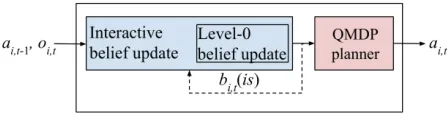
Figure 1: IPOMDP-net architecture overview. It embeds an interactive belief update algorithm and the QMDP planner, the hidden state encodes the interactive belief of agenti.
An IPOMDP-net consists of three main network modules as shown in Figure 1. The first two modules (blue boxes) perform interactive belief update using a customized particle filter for intentional models (Han and Gmytrasiewicz 2018). The interactive belief update module uses the level-0 belief update as a sub-module when the nesting levellbottoms out at 0. The third module (red box) represents the QMDP algo-rithm, which chooses the action given the current belief. Be-sides being a planning network, all modules of IPOMDP-net are differentiable, allowing the entire network to be trained end-to-end.
Network Architecture
The intuition behind embedding the I-POMDP model and the QMDP algorithm in a single, differentiable neural net-work is the neural analogy of linear and maximum oper-ations used in the related computoper-ations. Namely, the ma-trix multiplications and summations can be represented by convolutional layers and maximum operations can be repre-sented by max-pooling layers.
Below we will give some details on the individual mod-ules. For simplicity, assume there are two agent iandj in the game and the strategy level is 1. Consider the two-agent tiger game (Gmytrasiewicz and Doshi 2005), which general-izes the classic single agent tiger game (Kaelbling, Littman, and Cassandra 1998) to multi-agent settings. Two agents are standing in front of two doors. There are a tiger and a pile of gold behind each door. The agents take turns to open doors, they get rewards for getting the gold or penalties for fac-ing the tiger. They can choose to hear for further informa-tion about the tiger’s locainforma-tion, but their hearing is imperfect and they can not directly observe each other’s actions. In the I-POMDP formation, it is defined as: ISi,1 = S ×Θj,0,
whereS ={tiger on the left (TL), tiger on the right (TR)}
andΘj,0 = {< bj(s), Aj,Ωj, Tj, Oj, Rj, OCj >}; A = Ai×Ajis the set of joint actions,{listen (L), open left door (OL) and open right door(OR)} × {L, OL, OR};Ωi:{growl from left (GL) or right (GR)} × {creak from left (CL), right (CR) or silence (S)};Ti=Tj :S×Ai×Aj×S →[0,1]; Oi:S×Ai×Aj×Ωi→[0,1];Ri:IS×Ai×Aj→R.
The IPOMDP-net works on a sampling-based repre-sentation of interactive belief state ISi,1 = S ×Θj,0.
For the tiger game, a sample of physical state can be simply denoted using one-hot vectors, for example [1,0] represents s=TL. A sample of j’s model can be represented as a vector of length eight, for example θj = h0.5,0.67,0.5,0.85,0.5,−1,−100,10i, by param-eterizing j’s belief (0.5), and transition (0.67,0.5), ob-servation (0.85,0.5), and reward functions (−1,−100,10) (see (Han and Gmytrasiewicz 2018) for details). Thus, an example of initial ISi,1 samples can be a 2D vector
[1,0],[0.5,1.0,0.5,0.85,0.5,−1,−100,10].
Interactive belief update module.The core structure of the IPOMDP-net is the interactive belief update module, which is a neural implementation of the sampling based Interactive Belief Update algorithm described in (Han and Gmytrasiewicz 2018). It consists belief propagation, weight-ing accordweight-ing to both agents’ observations, reweighweight-ing and re-sampling. This module embeds both agentiandj’s mod-els as network weightsw. The output of this module will be the input of QMDP planner module.
The interactive belief update module maps agent i’s in-teractive belief, action, and observation to a next belief, bt
i,l = SE(b t−1
i,l , a t−1
i , o t
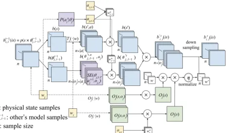
cor-(a) Interactive belief update module
(b) Level-0 belief update module
(c) QMDP planner module
Figure 2: IPOMDP-net consists of three modules
rects and normalizes the prediction (Equation 7).
ˆ
bti,l(ist) = X
ist−1
bi,l(ist−1)
X
atj−1
P r(atj−1|θtj,l−1−1)
×T(st−1, at−1, st)X
ot j
Oj(st, at−1, otj) (6)
×τ(btj,l−1−1, ajt−1, otj, bt,l−1)
bti,l(ist) =αX
atj−1
Oi(st, at−1, oti)ˆb t i,l(is
t) (7)
Equation 6 is implemented using convolutional layers and sub-modules. Firstly, agenti’s belief,b(isti,−11 ) =p(s, θj,t−10 ), will be divided intosandθtj,−10 . The first dimensionsis con-voluted with transition function Ti(·|w)with|A| convolu-tional filters. The kernel weights are parameters of the tran-sition functionTi(·|w). The output of the convolutional layer is aD1×D2×n× |A|tensor, whereD1andD2are the
sizes of the state space,nis the total number of belief sam-ples, and |A| = |Aj ×Aj|is the number of unique joint actions ofiandj. We stack different input samples together as channels of the convolutional layer. For instance, for the two-agent tiger game, the predicted physical state after con-volution is a1×2×100×9tensor, where the state samples are1×2(either[1,0]or[0,1]), and there are 9 total joint actions (|L, OL, OR| × |L, OL, OR|) and we assume 100
samples are used.
Elements of the second dimension of isti,−11 , the sam-ples of the other agent j’s model θtj,−10 , are the in-puts into the level-0 belief update module (btj,0 =
SE(btj,−10 , atj−1, ot
j) in Figure 2(b)). They will be up-dated to a new belief according to the particular model parameters of j. For example, j’s model sam-ple[0.5,1.0,0.5,0.85,0.5,−1,−100,10]in tiger game will be updated to [0.85,1.0,0.5,0.85,0.5,−1,−100,10]. Es-sentially, only the first parameter will be updated from bj(s=T L)=0.5 tobj(s=T L)=0.85
as it represents j’s be-lief about tiger being on the left, which corresponds to the τ(btj,l−1−1, atj−1, ot
j, bt,l−1)function in Equation 6. The belief
update ofjis for any possible actionajand anticipated ob-servationsoj, so there are totallyn×|oj|×|aj|sub-modules being used.
Since ˆbt
i,1(st, a) after convolution encodes predicted
physical belief after taking each of the joint actions, a ∈
A = Ai ×Aj, we need to select the belief correspond-ing to the last joint action. In Figure 1(a), notice that the wi and wj contain all the parameters of both i and j’s models, thus we compute j’s optimal actions according to j’s model,P(atj|θtj−1).P(atj|θjt−1)can be any single-agent POMDP solver, in this case we plug in a pretrained QMDP-net (Karkus, Hsu, and Lee 2017) to make the entire QMDP-network end-to-end. Then we use the soft indexing similar to the one used in QMDP-net (Karkus, Hsu, and Lee 2017), where wa
t−1is the indexing vector, a distribution overA. Then we
weightˆbti,1(st, a)bywta−1:
ˆbt i,l(st) =
X
a∈A
ˆ
bti,l(st, a)wta−1 (8)
Similarly,ˆbt
i,1(θj,t0, a)after level-0 belief update encodes
predicted models ofj after taking each ofj’s actions,a ∈
Aj, we select the belief corresponding toj’s last action us-ing soft indexus-ing again. Nowwaj
t−1is the indexing vector, a
distribution overAj, andˆbti,1(θj,t0, aj)is weighted byw aj
t−1:
ˆbt i,l(θ
t j,l−1) =
X
aj∈Aj ˆbt
i,l(θ t
j,l−1, aj)w aj
t−1 (9)
After updatingj’s model samples, we joinˆbt
i,1(st)and ˆ
bti,1(θtj,0)together to get the propagatedˆbti,1(ist). Namely,
the physical state samples ˆbti,1(st) are duplicated by the number of anticipated observations ofj and attached with correspondingˆbt
i,1(θj,t0). Thus, the number of initial belief
is to correct this predicted belief with both agents’ observa-tions.
Oj(s, oj) encodes observation probabilities for each of j’s observations, it is aD1×D2× |Oj|tensor. Similarly, Oi(s, oi)encodes observation probabilities for each of i’s observations, it is aD1×D2×|Oi|tensor. The initial weights of belief samplesw(b0
i)is uniformly initialized as1/|n|and then weighted by anticipated observations ofj and actual observation ofi. We select the observation function corre-sponding toi’s last observation using soft indexing again:
Oi(s) =
X
a∈A
Oi(s, oi)wto−1 (10)
The remaining step is a simple down-sampling according to the updated weights. After the resampling step, the number of predicted samples ofihas reduced fromn× |oj|back to n.
Level-0 belief update module. When the nesting level bottoms out, i.e. l = 0, this module updates the belief of the agent at level 0, and is used by interactive belief update module at a higher level. For example, in the tiger game, if agent i is at level 1,i modelsj as a level-0 POMDP and uses this module to computebi,1(θj,0) =bi,1(bj,0(s),θˆj,0).
Thus,j’s beliefbj,0(s)will be updated in the same way as
that in a single-agent POMDP. As shown in Equation 11 and 12, the two classic steps are the prediction through transition and the correction using observation.
ˆbt j(s
t) = X
st−1∈S
T(st−1, atj−1, s)btj−1(st−1) (11)
bjt(st) =αO(st, ajt−1, otj)ˆbtj(st) (12)
This module is implemented almost identically to the belief update (filter) module in the QMDP-net (Karkus, Hsu, and Lee 2017), except that the transition functionTjand obser-vation functionOjare also input arguments frombi,1(θj,0).
Here we refrain from repeating the explanation, but the basic idea is to represent the matrix multiplication in Equation 11 as a convolutional layer, use soft indexing to selectaj and oj, and make element-wise multiplication in Equation 12.
QMDP planner module. The QMDP planner
approxi-mates the I-POMDP value iteration by solving the under-lying MDP model, assuming the state is fully observable, and making one-step look-ahead search on the MDP values weighted byi’s beliefs. Actions are then chosen according to the weighted Q values. It is similar to QMDP planner in the QMDP-net, except thati’s interactive belief (i.e. output of the interactive belief update module) needs to be marginal-ized over all possible models ofj.
Qi,k+1(s, ai) =Ri(s, ai) +γ
X
s0
Ti(s, a, s0)Vi,k(s0) (13)
Vi,k(s) = max ai
Qi,k(s, ai) (14)
The value iteration in Equation 13 and 14 is implemented using convolutional and max pooling layers(Tamar et al. 2016;?). TheQi(s, ai)is aD1×D2× |Ai|tensor. Equa-tion 13 is implemented as a convoluEqua-tional layer followed by
an addition with Ri(s, ai), the kernel weights encode the transition functionTi. Equation 14 is implemented as a max-pooling layer withQi,k(s, ai)as input andVi,k(s)as output. K iterations of value updates are implemented as recur-rent layers representing Equation 13 and 14 K times with tied weights. AfterK iterations, the approximate Q values for each state-action pair are weighted byi’s belief about the physical state (Equation 16). But before that, since i’s interactive belief contains j’s models as well, we need to marginalize over models ofj(Equation 15). Finally, we se-lect the action that has the highest q-values.
bi,t(s) =
X
θj
bi,t(is) (15)
Qi(bi, ai) =
X
s
Qi,K(s, ai)bi,t(s) (16)
Training Algorithm
We train the IPOMDP-net in a reinforcement learning set-ting following the similar way in DQN (Mnih et al. 2015) (Algorithm 1). Due to partial observability, we use belief state instead of physical state in the experience replay mem-ory[bi,t, ai,t, ri,t+1, bi,t+1]. To update the network
param-eters w and back propagate the errors, we define the loss function as the mean squared error between the Q-value of the target and the IPOMDP-net. Immediate rewards are as-sumed obtainable and agenti’s belief is computed in the be-lief update module. We have also used the-greedy strategy to ensure adequate explorations of the belief space, espe-cially when the underlying planner is QMDP.
Algorithm 1: IPOMDP-net Training
1 Initialize belief state, replay memory, nesting levell 2 Initialize the networks with random weightsw 3 for episode= 1toM:
4 Initializeai,0and getoi,1
5 fort= 1toT:
6 sampleatj ∼P(Aj|θj,l−1)
7 select a random actionai,twith probability 8 otherwise selectai,t= arg maxaQ(bi,t, ai;w) 9 execute actionai,t, obtain rewardri,t, observa-tionoi,t+1, and updated beliefbi,t+1
10 store[bi,t, ai,t, ri,t+1, bi,t+1]in replay memory
11 randomly sample a minibatch in replay mem-ory[bi,m, ai,m, ri,m+1, bi,m+1]
12 compute the target Q-valueym=
ri,m if i+1 is terminal step
ri,m+βmaxaiQˆ(bi,m+1, ai
0;w−) otherwise
13 perform gradient descent on: (ym − Q(bi,m, ai,m;w))2
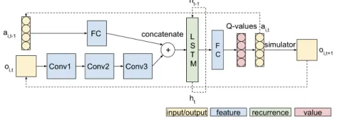
Figure 3: One time slice of ADRQN. Inputs areai,t−1and
oi,t, outputs are ai,t and oi,t+1. FC stands for fully
con-nected layer. Conv stands for convolutional layers. Output of LSTM layerhtwill be input into LSTM in the next time slice. Actual hyper parameters vary on different problems.
deep recurrent Q-network (ADRQN) for single-agent do-main (Zhu et al. 2018).
As shown in Figure 3, this network is a dual-modal hy-brid architecture that learns from the action and observa-tion histories, i.e.[ai,0, oi,1],[ai,1, oi,2], ...,[ai,t−1, oi,t]. The time series of action-observation pairs are integrated by an LSTM layer that extracts features (from these pairs) and learns the latent states. Then a fully connected layer com-putes Q-values based on the learned latent states. These la-tent states integrate the information contained in action and observation histories. It has been shown that the ADRQN outperforms the ARQN (Zhu et al. 2018), which outper-forms the DQN (Mnih et al. 2015). Thus, it is one of the state-of-the-art model-free networks for sequential decision making problems.
Training the ADRQN is similar to training the DQN except the experience replay memory now changes from
[st, ai,t, ri,t, si,t+1] to
{ai,t−1, oi,t}, ai,t, ri,t, oi,t+1
due to partially observability. Training ADRQN also converts a learning problem to a high-dimensional non-convex func-tion optimizafunc-tion (on the network weight w space). How-ever, besides model-embedding and network architecture, the major difference between IPOMDP-net and ADRQN is that weights in the IPOMDP-net encode both agents’ model parameters, but in ADRQN the weights are from another pa-rameter space.
Experiments
Experimental setup
The goal of the experiments is to verify that embedding models of other agents in the planning network benefits our decision-making. We want to understand the benefits in terms of the policy quality and generalizability. Since IPOMDP-net is a neural approximation to the symbolic I-POMDP, we also want to know how close this approxima-tion is in terms of planning performance.
We firstly test the planning performance of IPOMDP-net by comparing it with its symbolic counterpart. We initialize weights of the IPOMDP-net using true parameters of model functions and test it in various but fixed environments. In this planning setting, the reinforcements are unobservable and model functions are known. We show related results in
Table 1.
Then we apply the same IPOMDP-net architecture in model-based reinforcement learning (RL) problems, where there are two phases of experiments: training and test-ing. The training phase is for different neural networks (IPOMDP-net and ADRQN) to be trained, starting from ran-domly initialized weights and observable reinforcements, so that the converged networks are approximations to true pol-icy functions. The testing phase is to evaluate the trained networks in a planning setting where the rewards are unob-servable. We show related results in Table 2.
Therefore, we designed experiments of five problems in two categories. In the first category, we use the two-agent tiger game (Gmytrasiewicz and Doshi 2005) and UAV lem (Doshi and Gmytrasiewicz 2009), in which the prob-lem environments are small and fixed. The neural networks are trained on the same, fixed environment, and then applied back to it for testing. In the second category, we use three variations of the Maze problem (Russell and Norvig 2016) with size4×4,10×10, and16×16, in which the agentj tries to reach the goal whileitries to reach the goal and / or catchj. We want to evaluate if the model-free networks can keep up with model-based net and the IPOMDP-net learned in smaller environments (10×10) can generalize to larger ones (16×16). In these Maze variations, the loca-tions of the start, goal and obstacles are random in each of the training and testing maps.
Results and Discussions
Table 1: Average results for planning tasks. The IPOMDP-net with preassigned weight performs almost the same as it symbolic I-POMDP counterpart. The results are averaged over 50 random runs.
IPOMDP-net I-POMDP I-POMDP SARSOP
Tiger 2.25±0.11 2.26±0.09 2.32±0.15
UAV 9.10±0.39 9.09±0.45 9.27±0.52
Maze 4×4 0.17±0.05 0.16±0.06 0.19±0.04 Maze 10×10 -0.53±0.09 -0.56±0.08 -0.49±0.07 Maze 16×16 -0.99±0.10 -0.96±0.09 -0.81±0.10
In Table 1, we use known model parameters to preas-sign IPOMDP-net weights, the corresponding symbolic I-POMDP (with QMDP planner) is shown in the second col-umn. In the last column, we also report additional results on the symbolic I-POMDP using SARSOP planner (Kur-niawati, Hsu, and Lee 2008) instead of QMDP, which rep-resents the best performance that a symbolic approach can achieve now. We will look into ways of implementing SAR-SOP or other planners in IPOMDP-net, which generally re-quires more sophisticated network design.
We see that in all problems, the performance of pre-initialized IPOMDP-net is almost identical to the symbolic I-POMDP, which is to be expected as they are the neural and symbolic implementations of the same I-POMDP frame-work.
Table 2: Average rewards for different RL problems. The networks start from random weights. The results are aver-aged over 50 random runs.
(a) The learning and testing environments are fixed for Tiger and UAV. The performance difference is small.
Fixed environments
Tiger UAV
ADRQN 1.29±0.35 8.98±0.97
IPOMDP-net w/ trained weights 1.32±0.29 9.19±0.72
(b) In three maze tasks, the learning maps are randomly generated and testing maps are new, unseen ones. The performance of the model-free ADRQN degrades faster as maps size increases.
Random environments - Maze 4×4 10×10 16×16 ADRQN 0.12±0.08 -0.73±0.17 -1.58±0.39 IPOMDP-net trained 0.18±0.05 -0.52±0.10 -0.88±0.21
of the model-free ADRQN degrades faster as maps size in-creases from 4×4 to 16×16.
IPOMDP-net learns policies that generalize to new en-vironments.In the fixed Tiger and UAV environments (Ta-ble 2(a)), the model-free ADRQNs have compara(Ta-ble perfor-mance to the IPOMDP-net. The reason is that in a fixed en-vironment, a network may directly learn the mapping from features to policy. In contrast, the IPOMDP-net learns a model for planning, i.e. generating a near-optimal policy for arbitrary environments. For the4×4Maze problem, we ran-domly generate 1100 maps and divide them into training and testing sets of size 1000 and 100. For the10×10Maze, there are 5000 maps for training and 200 for testing. We see that in the first and second columns of Table 2(b), the average rewards of IPOMDP-net are higher than the ADRQN.
IPOMDP-net policies learned in small environments transfers directly to larger ones. For the 16×16 Maze problem, we directly apply the IPOMDP-net trained in10×
10mazes and increase the value iteration recurrenceKto40
and keeping all other parameters unchanged. For the trained ADRQNs in10×10mazes, we also increased the recurrence of LSTM layers to20. Although the map size is larger, the underlying planning nature is the same as in smaller mazes. We see that the IPOMDP-net is significantly better than the model-free ADRQN, the performance of ADRQN degrades fast when the maze size increases.
IPOMDP-net learns an overall better policy instead of a “true” model.It makes sense that the learned model should be the ground truth if the embedded I-POPMDP al-gorithm is exact. Since our planning alal-gorithm is QMDP, the learnedT(·|θ),O(·|θ), andR(·|θ)does not necessarily rep-resent the true transition, observation, and reward functions. The reason is that the end-to-end training gives IPOMDP-net the opportunity to learn an “incorrect” but useful model that compensates the limitation of the approximation algorithm, the QMDP.
Visualization
We visualize the learned value function of agent i for the
16×16Maze problem. In Figure 4(b), we seeiassigns high values over the target andj’s locations, but the target loca-tion is “hotter” thanj’s location. This is because thatjtends to move a lot, and therefore, its location is not as valuable as the goal (catchingjor reaching target location gives the same+1 reward). In Figure 4(c), sincej is modeled as a level-0 POMDP agent, he has no clue abouti’s existence. Thus, inj’s reward function, states close to the goal have high values.
(a) (b) (c)
Figure 4: Visualization of both agents’ value functions on Maze 16× 16 problem: (a) a particular game map, (b) learned value function of i on one sample state ( whenj at the orange square position), (c) learned value function of j. Black squares are obstacles, red isi’s location, orange is j’s location, and blue is the target location.
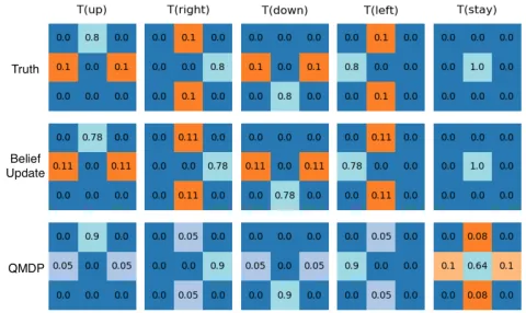
Figure 5: The learned transitions in belief update module and QMDP module are different. The first row is the ground truth. The second row is the transition in belief update mod-ule. The third row is the transition in QMDP modmod-ule.
Conclusion
We have described the IPOMDP-net, a neural network archi-tecture for multi-agent planning under partial observability. It combines model-free learning and model-based planning by embedding an I-POMDP model and a QMDP planning algorithm in a network learning architecture. We show its effectiveness, performance, and generalizability on various problems. Our approach provides a general, model-based neural computing architecture for multi-agent planning.
One future research direction is to implement the exact I-POMDP value iteration instead of the QMDP approxima-tion. The first step shall be an implementation of single-agent POMDP value iteration, which is straightforward as it only involves linear matrix operations and maximum op-erations. The real challenge is to find the most appropriate way to represent the value function on the nested interactive belief structures. Currently one major constraint of our work is the scalability when there are multiple agents or the input size / problem state is huge. This may lead to another direc-tion, which is an attention mechanism (Tamar et al. 2016) to reduce the effective number of network parameters, because in many problems, the importance and effects of neighbor-ing states might be contextually dependent on what is the current state.
References
Ciregan, D.; Meier, U.; and Schmidhuber, J. Multi-column deep neural networks for image classification. In2012 IEEE Conference on Computer Vision and Pattern Recognition.
Doshi, P., and Gmytrasiewicz, P. J. 2009. Monte Carlo sampling methods for approximating interactive POMDPs.
Journal of Artificial Intelligence Research34:297–337.
Farabet, C.; Couprie, C.; Najman, L.; and LeCun, Y. 2013. Learning hierarchical features for scene labeling. IEEE transactions on pattern analysis and machine intelligence
35(8):1915–1929.
Gmytrasiewicz, P. J., and Doshi, P. 2005. A framework for sequential planning in multi-agent settings. J. Artif. Intell. Res.(JAIR)24:49–79.
Han, Y., and Gmytrasiewicz, P. J. 2018. Learning others’ intentional models in multi-agent settings using interactive POMDPs. InThe Workshops of the The Thirty-Second AAAI Conference on Artificial Intelligence., 666–673.
Hausknecht, M., and Stone, P. 2015. Deep recurrent Q-learning for partially observable MDPs. InAAAI 2015 Fall
Symposium.
Hochreiter, S., and Schmidhuber, J. 1997. Long short-term memory.Neural computation9(8):1735–1780.
Kaelbling, L. P.; Littman, M. L.; and Cassandra, A. R. 1998. Planning and acting in partially observable stochastic do-mains. Artificial Intelligence101(1):99–134.
Karkus, P.; Hsu, D.; and Lee, W. S. 2017. QMDP-Net: deep learning for planning under partial observability. In
Advances in Neural Information Processing Systems, 4697– 4707.
Krizhevsky, A.; Sutskever, I.; and Hinton, G. E. 2012. Imagenet classification with deep convolutional neural net-works. InAdvances in neural information processing sys-tems, 1097–1105.
Kurniawati, H.; Hsu, D.; and Lee, W. S. 2008. SARSOP: ef-ficient point-based POMDP planning by approximating op-timally reachable belief spaces. In Robotics: Science and systems, volume 2008. Zurich, Switzerland.
Levine, S.; Finn, C.; Darrell, T.; and Abbeel, P. 2016. End-to-end training of deep visuomotor policies. The Journal of
Machine Learning Research17(1):1334–1373.
Mnih, V.; Kavukcuoglu, K.; Silver, D.; Rusu, A. A.; Ve-ness, J.; Bellemare, M. G.; Graves, A.; Riedmiller, M.; Fidjeland, A. K.; Ostrovski, G.; et al. 2015. Human-level control through deep reinforcement learning. Nature
518(7540):529.
Russell, S. J., and Norvig, P. 2016. Artificial intelligence: a modern approach. Malaysia; Pearson Education Limited,. Tamar, A.; Wu, Y.; Thomas, G.; Levine, S.; and Abbeel, P. 2016. Value iteration networks. InAdvances in Neural In-formation Processing Systems, 2154–2162.