ISSN 0097-8078, Water Resources, 2007, Vol. 34, No. 2, pp. 163–170. © Pleiades Publishing, Ltd., 2007.
Original Russian Text © A. Voinov, R. Costanza, C. Fitz, Th. Maxwell, 2007, published in Vodnye Resursy, 2007, Vol. 34, No. 2, pp. 181–189.
INTRODUCTION
The modular approach takes advantage of the Spa-tial Modeling Environment [1] that allows integration of various Stella models and C++ user code, and embeds local simulation models into a spatial context. Local ecosystem dynamics are replicated across a grid of cells that compose the rasterized landscape. Differ-ent habitats and land use types translate into differDiffer-ent modules and parameter sets. Spatial hydrologic mod-ules link the cells together. These are also part of the LHEM and define horizontal fluxes of material and information.
The General Ecosystem Model (GEM) [2] has been designed to simulate a variety of ecosystem types using a fixed model structure, in hope that the generic nature of the model will help alleviate the “reinventing-the-wheel” syndrome of model development. While the GEM approach still seems to be extremely important for cross ecosystem and scale comparisons, it turned out to be somewhat insufficient to cover all the possible variety in ecosystem processes and attributes that come into play when going from one ecosystem type to another, and from one scale to another. Modeling is a goal driven process, and different goals in most cases will require different models. There is too much eco-logical variability to be represented efficiently within the framework of one general model. Either something important gets missed, or the model becomes too redundant to be handled efficiently especially within the framework of larger spatially explicit models. Sim-ilarly, when changing scale and resolution different sets of variables and processes come into play. Certain pro-cesses that could be considered at equilibrium at a
weekly time scale need be disintegrated and considered in dynamic at an hourly time scale. For example, pond-ing of surface water after a rainfall event is an important process at fine temporal resolution, but may become redundant if the time step is large enough to make all the surface water either removed by overland flows, or infiltrated. Daily net primary productivity fluctuations, that are important in a model of crop growth, may be less important in a forest model that is to be run over decades with only average annual climatic data avail-able. Once again the general approach may result in either insufficiency or redundancy.
The modular approach is a logical extension of the general approach. In this case instead of creating a model general enough to represent all the variety of ecological systems under different environmental con-ditions, we develop a library of modules simulating var-ious components of ecosystems or entire ecosystems under various assumptions and resolutions. In this case the challenge is to put the modules together, using con-sistent and appropriate scales of process complexity, and make them talk to each other within a framework of a full model. The concept of modularity gained strong momentum with the wide spread of the object oriented approach in software development [3, 4].
One of the important features of the Spatial Model-ing Environment (SME) [5] is that it can take individual STELLA [6] models and translate them into a format that supports modularity. In addition to STELLA mod-ules, SME can also incorporate user-coded modules that are essential to describe, say, various spatial fluxes in a watershed or a landscape. Instead of a general model that should represent all the variety of
ecosys-HYDROPHYSICAL PROCESSES
Patuxent Landscape Model: 1. Hydrological Model Development
A. Voinov, R. Costanza, C. Fitz, and T. Maxwell
Gund Institute for Ecological Economics, University of VermontBurlington, Main Street 590, VT 05405-0088
Received March 25, 2004
Abstract—We developed a spatially explicit, process-based model of the 2352 km2 Patuxent river watershed in Maryland, and its subwatersheds to integrate data and knowledge over several spatial, temporal and complex-ity scales, and to serve as an aid to regional management. The model was developed using the Library of Hydro-Ecological Modules (LHEM, http://giee.uvm.edu/LHEM), which was designed to create flexible landscape model structures that can be easily modified and extended to suit the requirements of a variety of goals and case studies. The LHEM includes modules that simulate various aspects of ecosystem dynamics. In this paper we consider modules that represent the physical conditions in the environment (climatic factors, geoporphology), and hydrologic processes, both locally and spatially. Where possible the modules are formulated as Stella(R) models, spatial transport processes are presented as C++ code.
164 VOINOV et al.
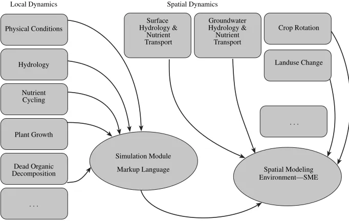
tems, by using SME we can formulate a general modu-lar framework (Fig. 1), which defines the set of basic variables and connections between the modules. Partic-ular implementations of modules are flexible and assume a wide variety of components that are to be made available through libraries of modules. The mod-ules are formulated as stand-alone STELLA models that can be developed, tested and used independently. However they can share certain variables that are the same in different modules, using a convention that is defined and supported in the library specification table. When modules are developed and run independently, these variables are specified by user-defined constants, graphics or timeseries. Within the SME context these variables get updated in other modules to create a truly dynamic interaction.
For example, spatial dynamics modules can be for-mulated in C++. They can use some of the SME classes to get access to the spatial data and can then be incor-porated into the SME driver and used to update the local variables described within the STELLA modules. In this case it is hard to offer the same level of transpar-ency as with the STELLA modules. More emphasis should be made on explicit documentation and com-ments to the code. We also hope that by presenting the various modules of the LHEM on the web and offering detailed description of various modules and their func-tions we can increase their utility for reuse and further improvement.
In this and three following papers we will give a brief description of the major modules that are cur-rently included into the LHEM and that were used to put together the Patuxent Landscape Model (PLM)—a fairly complex spatial watershed model and that was
developed to integrate the ecological and socio-eco-nomic dynamics in a watershed. This paper is focused on general ideas of modular modeling and describes how physical conditions and hydrologic processes are presented in LHEM.
GENERAL CONVENTIONS
In SME, local modules can be described as Sectors in STELLA. Each module is a different STELLA model. In what follows we will call state variables, forcing functions and parameters simply variables if they do not need be distinguished. The variables within a sector will be considered as owned by this module. All the external variables that are defined outside of the sector borders can be defined in other modules. Within a module, to make it operable as a stand-alone model, these external variables should be defined as constants or as timeseries (say, defined as graphs in Stella) that can change with time or as functions of some other independent variables.
Variables that are shared between modules should have the same name. The SME translator takes the STELLA equations saved as a text file, and translates them into an intermediate formalization, called the Modular Markup Language (MML) [5]. It will find the shared names and link them together. A config file will be produced that contains all the variables from all the modules. This config file can be further edited to change the values used for the variables in the driver. However these changes will not affect the values that the variables are set to in the STELLA formulations of the modules. Due to STELLA limitations there is no way back from MML or STELLA equations to the
Physical Conditions
Hydrology
Nutrient
Plant Growth
Dead Organic
. . .
Cycling
Decomposition
. . .
Local Dynamics Spatial Dynamics
Surface Hydrology &
Nutrient Transport
Groundwater Hydrology & Nutrient Transport
Crop Rotation
Landuse Change
Spatial Modeling Environment—SME Simulation Module
Markup Language
PATUXENT LANDSCAPE MODEL: 1. 165 STELLA icon based diagram and modeling tools.
Therefore all the changes that are made to the MML formulation or directly to the driver in C++ will be lost if we export and process a new STELLA equations file. Whereas most of the local dynamics can be effec-tively described within STELLA models, it becomes hard if not impossible to represent spatial processes using this formalism. To link individual local models into a spatial network, again, SME can be used, if the appropriate code is provided. The SME allows one to link C++ programs, described as User Code, with the local ordinary differential (difference) equations (ODE) generated based on STELLA formulations. A number of the SME classes are made available for writ-ing user code in order to provide access to spatial and non-spatial data structures handled by the SME.
Besides, as local dynamics get treated in the SME in a spatial context, it also gets the spatial variability that can be associated with the various parameters being spatially distributed, related to, say, soil or habitat types. In this case when moving from one spatial local-ity to another the same system of ODEs generated from STELLA gets to be solved with a different parameter set, one that is substituted by SME. Currently SME does not incorporate any extensive database features to serve the needs of describing and archiving the numer-ous parameters encountered in models and modules. However there are several well-elaborated input mech-anisms that allow one to read the location-dependent data from various file formats. For example, the habitat-dependent parameters are accumulated in a file that has various columns representing the different model parameters, and rows describing the various habitats. A parameter described as habitat-dependent in the con-fig.file is then input from this file based on the informa-tion about the particular habitat specified by the Land Use map.
PHYSICAL MODULES
Variables and major assumptions. There are no state variables in this module. The variables defined here are the forcing functions and parameters that describe the physical environment and include Climatic factors (precipitation, temperature, humidity, wind speed, solar radiation; surface geomorphology (eleva-tion, bathymetry, soils); auxiliary variables shared by other modules (day length, Julian day, and habitat type).
The module is designed mostly to simplify data pre-processing. It takes care of various conversions when the raw data are input into the model. For particular applications there is good chance that some modifica-tions will be required if the data available are presented in some different formats and units. In some cases, additional sub-modules may be formulated. For exam-ple the photoactive solar radiation (PAR) is rarely
avail-able in standard climatic data sets. In many cases this forcing function can be well estimated by empirical for-mulas based on the latitude of the study area.
Solar radiation. There are currently two modules in LHEM that calculate PAR. The first one is similar to the one used in GEM [2]. It is based on an algorithm derived from Nikolov and Zeller [7], that begins with a calculation of daily solar radiation at the top of the atmosphere based on Julian date, latitude, solar decli-nation, and other factors. Mean monthly cloud cover is calculated using a regressed relationship based on daily precipitation, humidity, and temperature. This monthly cloud cover value is used to attenuate the daily radiation reaching the surface. Daily radiation (PAR in cal/cm2 day)
received at the earth surface at a particular elevation, latitude, or time of year in the Northern hemisphere is calculated using the Beer’s law relationship to account for attenuation through the atmosphere.
The second algorithm is a simplification of the Nikolov and Zeller model that matches their results in mid-latitudes (20 < Lat < 64) almost exactly (r2 = 0.96).
The solar radiation at the earth surface is calculated using an empirical formula:
where A = 720.52–6.68 Lat; B = 105.94(Lat – 17.48)0.27;
C = 175 – 3.6 Lat, D is the cloudiness, and T_rad = 2/365 PI (DayJul – 173) is the conversion from days to radian.
HYDROLOGIC MODULES
Variables and major assumptions. The traditional scheme of vertical water movement [8], also imple-mented in GEM [2], assumes that water is fluxed along the following pathway: rainfall surface water water in the unsaturated layer water in the satu-rated zone. Snow is yet another storage that is impor-tant to mimic the delayed response caused by certain climatic conditions. In each of the stages some portions of water are diverted due to physical (evaporation, run-off) and biological (transpiration) processes, but in the vertical dimension the flow is controlled by the exchange between these 4 major phases: surface water (SW), snow/ice (SI), water in unsaturated storage (UW), and water in saturated storage (S).
We build our hydrologic module around these four state variables. These variables as well as the associ-ated fluxes are computed within this module and made available for input into other modules. On the input side for the hydrologic module we use: precipitation, air temperature, humidity, wind velocity, habitat type, soil type, slope, root depth, leaf area index, stream sin-uosidity.
PAR
166 VOINOV et al. In addition to the GEM hydrologic module that
proved to be well suited for wetland conditions, we have formulated another module that is better adjusted to terrestrial ecosystems and was used in PLM. Taking into account the temporal (1 day) and spatial (200 m, 1 km) resolution and the available input data, we have simplified the GEM module.
At a daily time step, the model cannot attempt to mimic the behavior of short-term events such as the fast dynamics of a wetting front, when rainwater infiltrates into soil and then travels through the unsaturated zone towards the saturated groundwater. During a rapid rain-fall event, surface water may accumulate in pools and depressions but in a catchment scale, over the period of a day, most of this water will either infiltrate, evaporate, or be removed by horizontal runoff. Infiltration rates based on soil type within the Patuxent watershed, range from 0.15 to 6.2 m/day [9], potentially accommodating all but the most intense rainfall events in vegetated areas. The intensity of rainfall events can strongly influ-ence runoff generation, but climatic data are rarely available for shorter than daily time steps. Also, if the model is to be run over large areas for many years, the diel rainfall data become inappropriate and difficult to project for scenario runs. Therefore, a certain amount of detail must be forfeited to facilitate regional model implementation.
With these limitations in mind, we have imple-mented the following conceptualization. We assumed that rainfall infiltrates immediately to the unsaturated layer and only accumulates as surface water if the unsaturated layer becomes saturated or if the daily infil-tration rate is exceeded. Ice and snow may still accumu-late. Surface water in the model is water in rivers, creeks, ponds, and the like. There is no standing surface water on top of unsaturated layer. Surface water is removed by horizontal runoff or evaporation. Within the one-day time step, surface water flux also accounts for the shallow subsurface fluxes that rapidly bring the water distributed over the landscape into the micro channels and eventually to the river. Thus, the surface water transport takes into account the shallow subsur-face flow that may occur during rainfall, allowing the model to account for the significantly different nutrient transport capabilities between shallow and deep sub-surface flow. Conceptually this is similar to the slow and quick flow separation [10, 11] assumed in empiri-cal models of runoff. In this case the surface water vari-able accounts for the quick runoff, while the saturated storage performs as the slow runoff, defining the base-flow rate between rainfall events.
The following processes are analyzed within this module and therefore may be available in the other modules.
Interception
A certain part of rainfall gets attached to vegetation or other structures on the landscape and further evapo-rates without even reaching the ground. The net inter-ception loss is typically 10 to 30% of rainfall [12], and depends both on the canopy storage capacity and the nature and pattern of the rainfall, since up to half of the evaporation of the intercepted water occurs during the storm itself. Therefore we assume that the amount of water that the vegetation can intercept is in proportion to the total biomass:
HI= max(ε1R, ε2Lr),
where Lr is the leaf area index (LAI); ε1 is the habitat
dependent landscape interception parameter; ε2 is the
vegetation interception parameter, and R is the amount of rainfall (mm). In this way a certain amount is inter-cepted for any precipitation event and only the remain-ing part is delivered to the ground.
Evaporation and Transpiration
As in GEM, pan evaporation from surface water,
HE, (m day–1) is calculated according to the Chris-tiansen model [13]. The model uses temperature (T), solar radiation (I), wind speed (W) and humidity (H) as the independent variables.
Evapotranspiration is the process that removes water from the ground and releases it into the atmo-sphere. In addition to the evaporation process that is responsible for the air-water interface, we also account for the delivery process that makes water available for evaporation. If the surface is vegetated then the biolog-ical process of transpiration, that is performed by plants using water from the root zone, brings water to the leaves, pushing it out through the leaf stomatal pores and making it available for evaporation. If there are no plants, ponded water or soil moisture is evaporated.
The portion of land that is covered by vegetation can be approximated by the leaf area index, Lr The total amount of evapotranspiration is then
HT = LrTR + (1 – min(1, Lr))E,
Here E = CeHEUr is the evaporation from the ground,
Ce is the ground evaporation rate, HE is the pan evapo-ration for open water defined above, and Ur is the rela-tive moisture proportion (Ur = U/P, where U is the mois-ture proportion and P is the porosity). When the leaf area index is larger than 1, the ground evaporation pro-cess shuts down, and TR, total transpiration, becomes predominant. TR is further subdivided into transpira-tion from the unsaturated (TRu) and saturated (TRs) lay-ers:
TR = TRu + TRs = θvTR + (1 – θv)TR,
where TR is the transpiration, and θv is the proportion
PATUXENT LANDSCAPE MODEL: 1. 167
where UWd is the depth of the unsaturated layer, Rd is the root zone depth, R0 is the distance to the saturated
layer at which the capillary effect becomes pro-nounced, Rexp is the index of the capillary root suction
from the saturated layer that effectively makes satu-rated water available even when the roots are not yet long enough to reach it (UWd > Rd):
Rexp = exp(–10(UWd – Rd)).
Wa is the water availability index:
that makes water fully available when unsaturated moisture proportion U is larger than drying capacity Ud, which is usually 50-60% of field capacity Uf, it makes water unavailable when U is less than the wilting point
Uw, (may be assumed equal to 10% of field capacity), and it returns an intermediate value otherwise. This is further modified by the capillary action, potentially making water available even when the unsaturated zone is totally dry, but the roots are close to the saturated storage.
For potential transpiration íRp we have imple-mented the Penman-Monteith resistance based model of evapotranspiration, which is currently considered most advanced in hydrologic practice. The equation is fairly complex and is well documented in the literature [12]. It represents the amount of water that is lost into the atmosphere as a function of climatic conditions (tem-perature, humidity, solar radiation, wind velocity), and vegetation characteristics, such as the LAI.
Transpiration is then calculated from potential tran-spiration, by taking into account the water availability Wa:
TR = CtrTRpWa,
where Ctr is the habitat dependent transpiration rate, and TRp is the Penman–Monteith transpiration.
Evapotranspiration is probably one of the most com-plicated processes in the hydrologic cycle; therefore it is also implemented as a separate module in the LHEM.
Infiltration
Since the model is run on a daily basis and since we assume that rainfall infiltrates immediately into the
ϑv
WaUWd/ R( d+Rexp),if Rd+R0>UWd
1 if, Rd+R0<UWd
0 if, UWd = 0,
⎩ ⎪ ⎨ ⎪ ⎧
=
Wa = 1 ,Rexp
0 if, U<Uw
1 if, U>Ud U–Uw
( )/(Ud–Uw),
otherwise
⎩ ⎪ ⎪ ⎨ ⎪ ⎪ ⎧
+
⎝ ⎠
⎜ ⎟
⎜ ⎟
⎜ ⎟
⎜ ⎟
⎜ ⎟
⎛ ⎞
,
unsaturated layer, infiltration is defined by the potential infiltration and by the unsaturated storage that is cur-rently available for water intake (unsaturated capacity). Surface features characterize potential infiltration:
Ip = CHabCS/CSI,
where CS (m/day) is the infiltration rate for a given type of soil, CHab is the habitat type modifier (0 < CHab < 1),
and CSI (degrees) is the slope modifier.
The unsaturated capacity is the total volume of pores in the soil that is not yet taken by water:
Uc = UWd(P – U),
where P is the soil porosity. If Ip is less than the unsat-urated capacity then the potential infiltration is realized and the actual infiltration HF = Ip. If Ip > Uc then the incoming water will fill up all the pores, effectively eliminating the unsaturated zone and making it satu-rated. Therefore in this case we channel all the infil-trated flow to the saturated storage, add the available unsaturated water to it and set UW = 0. Whatever water is left after infiltration is surface water that is available for horizontal runoff.
Percolation
By gravitational force, a certain amount of water percolates from the unsaturated storage further down until it hits the saturated layer. Only the water that is in excess of field capacity is available for percolation. When the unsaturated moisture proportion is below field capacity, capillary and adhesive forces retain all the water. Therefore the amount of water available for percolation is:
Ue = U – Uf,
and the percolation rate is defined by the equation:
where Cvc is the soil dependent vertical hydraulic
con-ductivity parameter.
In addition to the percolation process, additional water is transferred from the unsaturated layer to the saturated layer whenever the water table is moving up. In this case, water that is kept in the pores of the unsat-urated layer is added to the water coming up from the saturated layer, further rising the saturated layer. This amount is equal to
HP0 = max(0, UDh),
where Dh = UWd(t) – UWd(t – 1), which is the change in unsaturated water depth over one time step.
Conversely, if the water table is going down, the moisture at field capacity stays in the soil and is added to the unsaturated storage:
HP1 = max(0, Uf, Dh). Hp 2CvcP*Ue
0.4
/ P( –Uf)
0.4
Ue
0.4
+
( ),
168 VOINOV et al.
Spatial Implementation
The algorithms involved in the spatial hydrologic modules have been discussed in more detail elsewhere [14, 15]. A major hypothesis that we are testing is that overland and channel flow can be modeled similarly. Traditionally, in most models of overland flow the sur-face water is moved according to two separate algo-rithms: one for the 2-dimensional flux across the land-scape and another for the 1-dimensional channel flow. This approach is used in some of the classic spatial hydro-logic models such as ANSWERS [16] or SHE [17]. How-ever, considering the spatial and temporal scale of the Patuxent model, as well as its overall complexity, we use a simplified water balance algorithm for both types of flow.
Given the cell size of the model (200 m or 1 km), we may assume that in every cell there will be a stream or depression present where surface water can accumu-late. Therefore it makes sense to consider the whole area as a linked network of channels, where each cell contains a channel reach which discharges into a single adjacent channel reach. The channel network is gener-ated from a link map, which connects each cell with its one downstream neighbor out of the eight possible nearest neighbors.
After the water head in each raster cell is modified by the vertical fluxes controlled in the unit model, the surface water and its dissolved or suspended components move between cells based on one of two algorithms being tested. In the simplified algorithm a certain fraction of water is taken out of a cell and added to a cell downstream. This operation is either iterated several (10–20) times a day, effectively generating a smaller time step to allow fast riv-erflow, or the location of the recipient cell is calculated based on the amount of head in the donor cell after which in one time step the full amount of water is moved over several cells downstream along the flow path determined
by the link map (Fig. 2). The number of iterations or the length of the flowpath needed for the hydrologic module are calibrated, so that the water flow rates match gage data [15].
Another algorithm stops water movement when the water heads in two adjacent cells equilibrate. We examine the flow between two adjacent cells as flow in an open channel and use the slope-area method [18], which is a kinematic wave approximation of St. Venant’s momentum equation. The flux (m3/d) in this case is described by the
empirical Manning’s equation for overland flow. The equation is further modified to ensure that there is no flux after the two cells equilibrate and then the flux rate is accelerated using the multicell dispersion algorithm dis-cussed in [14]. While the first algorithm works well for the piedmont area with significant elevation gradients, the second one is more appropriate for the coastal plain region where there are significant areas of low relief and tidal forces, which permit counterflows.
There are three major modules currently available to move water and constituents in the horizontal dimen-sion. SWTRANS1 and SWTRANS2 are used for sur-face water dynamics, GWTRANS—takes care of the aggregated saturated water storage. SWTRANS1 is mostly useful for relatively flat areas, such as wetlands, coastal plains, and estuaries. In this module backflow is allowed and the water level is calculated by equilibrat-ing the water in a number of adjacent cells [14]. The call to the function is:
SWTRANS1 (S_WATER, MAP, ELEVATION, STUFF),
where S_WATER is the map of surface water, also updated by the unit models; MAP defines the study area; ELEVATION is the elevation map; and STUFF is the map of constituent concentrations.
(‡) (b) (c)
PATUXENT LANDSCAPE MODEL: 1. 169 SWTRANS2 assumes that there is a
well-pro-nounced gradient in elevation that makes sure that water moves only in one direction. This is most appro-priate for terrestrial ecosystems, which can usually be described by a link map that clearly indicates in which direction the water is running [15]. The function call is similar to the above.
SWTRANSP is a combination of SWTRANS1 and SWTRANS2. Here water can either equilibrate in rela-tively flat areas or run downhill, where the gradient is dominant. This function is used for areas that have a combination of steep and flat regions. In this case another variable is added to the function call:
SWTRANSP (S_WATER, MAP, HABMAP, ELEVATION, STUFF).
HABMAP is the additional coverage that is used to decide where the first algorithm is more appropriate and where the second one should be used. In some cases it can be the Habitat Map, where cells in the Open Water category are the ones that need the equilibration algorithm.
GWTRANS calculates the fluxes of groundwater and updates the concentration of constituents in cells. The function is based on a modified Darcy formaliza-tion of the groundwater flow. For each cell the flux is determined as a function of saturated conductivity and water head difference between the current cell and the average head of the cell and its eight neighbors. We assume that one vertically homogenous aquifer inter-acts with the surface water. The call to the function is:
GWTRANS (SAT_WATER, POROSITY, H_CONDUCT, MAP, STUFF, UNSATW),
where SAT_WATER is the map of saturated water height, also updated by the unit models; POROSITY is the coverage for soil dependent porosities; H_CONDUCT is the coverage for specific horizontal conductivity coefficients, that may also be soil depen-dent, STUFF is the map of constituent concentrations, that can be Nitrogen or Phosphorus in this case; and UNSATW is the amount of water in unsaturated stor-age. H_CONDUCT is calculated as the cell-size weighted horizontal conductivity:
where A is the cell size and Ch is the conductivity. Firstly, the function calculates for each cell the average conductivity-weighted water stage for the nine cells that are the immediate vicinity of a cell and the cell itself:
Ω is the vicinity of cell (i, j), that consists of cells (i – 1,
j – 1), (i – 1, j), (i – 1, j + 1), (i, j – 1), (i, j), (i, j + 1), (i
+ 1, j – 1), (i + 1, j) and (i+1, j+1); (i + 1, j + 1); Sij—
H_CONDUCT = Ch A,
H0 SijCij/ PijCij, i j
∑
∈W i j∑
∈W=
SAT_WATER; Cij – H_CONDUCT; and Pij is POROSITY. Next it is assumed that the stage in the cell (i, j) will tend towards this equilibrium and for each of the pairwise interactions with the neighboring cells k the flow Fk is calculated:
Fk = (H0Pij – Sk) (Cij + Ck)/2, where k∈ Ω\(i, j).
The new stage is then Sij = Sij + ΣkFk. Note that when
Fk > 0 water is leaving the cell (i, j) and flows into the neighboring cell k. It flows in the opposite direction when Fk < 0.
The flow of water also carries the constituents (such as nutrients and sediments), whose concentration in cell (i, j) is updated with each of the pairwise flows calcu-lated:
Nij = Nij – Nij Fk/Sij, if Fk > 0; and
Nij = Nij + Nk Fk/Sij, if Fk < 0.
Here Nij is the amount of the constituent in cell (i, j), and Nk is the amount of constituent in the neighboring cells (k∈ Ω\(i, j)).
ACKNOWLEDGMENTS
The EPA STAR (Science to Achieve Results) pro-gram, Office of Research and Development, National Center for Environmental Research and Quality Assur-ance (R82716901), has provided funding for this research.
REFERENCES
1. Maxwell, T. and Costanza, R., Distributed Modular Spa-tial Ecosystem Modelling, International J. of Computer Simulation: Special Issue on Advanced Simulation Methodologies, 1995, vol. 5, no. 3, pp. 247–262. 2. Fitz, H.C., et al., Development of a General Ecosystem
Model for a Range of Scales and Ecosystems, Ecologi-cal Modelling, 1996, vol. 88, nos. 1/3, pp. 263–295. 3. Silvert, W., Object-Oriented Ecosystem Modeling.
Eco-logical Modelling, 1993, vol. 68, pp. 91–118.
4. Sequeira, R.A., Olson, R.L., and McKinion, J.M., Imple-menting Generic, Object-Oriented Models in Biology, Ecological Modelling, 1997, vol. 94, no. 1, pp. 17–31. 5. Maxwell, T. and Costanza, R., A Language for Modular
Spatio-Temporal Simulation, Ecological Modelling, 1997, vol. 103, nos. 2−3, pp. 105–114.
6. HPS, STELLA: High Performance Systems. 1995. 7. Nikolov, N.T. and Zeiler, K.F., A Solar Radiation
Algo-rithm for Ecosystem Dynamic Models, Ecological Mod-elling, 1992, vol. 61, pp. 149–168.
8. Novotny, V., Olem, H., Water Quality. Prevention, Iden-tification, and Management of Diffuse Pollution, NY: Van Nostrand Reinhold, 1994.
170 VOINOV et al. 10. Jakeman, A.J. and Homberger, G.M., How Much
Com-plexity Is Warranted in a Rainfall–Runoff Model, Water Resour. Res., 1993, vol. 29, no. 8, pp. 2637–2649.
11. Post, D.A. and Jakeman, F.J., Relationship Between Catchment Attributes and Hydrological Response Char-acteristics in Small Australian Mountain Ash Catch-ments, Hydrological Processes, 1996, vol. 10, pp. 877– 892.
12. Shuttleworth, W.J., Evaporation, in Handbook of Hydrol-ogy, New York: McGraw-Hill Inc, 1993, p. 4.1–4.53.
13. Saxton, K.E. and McGuinness, J.L., Evapotranspiration. In Hydrologic Modeling of Small Watersheds, Haan, C.T., Johnson, H.P., and Brakensiek, D., Eds., London: ASAE Monograph: St. Joseph, pp. 229–273.
14. Voinov, A., Fitz, C., and Costanza, R., Surface Water Flow in Landscape Models: 1. Everglades Case Study, Ecological Modelling, 1998, vol. 108, nos. 1−3, pp. 131– 144.