Proper Lucky Number of Hexagonal Mesh and Honeycomb Network

Proper Lucky Number of Hexagonal Mesh

and Honeycomb Network

D. Antony Xavier1, R.C. Thivyarathi2

1

Department of Mathematics, Loyola College, Chennai, India

2

Department of Mathematics, RMD college, Chennai, India

Abstract

:

Let 𝐺 𝑉, 𝐸 be a graph with vertex set 𝑉 and edge set E . Let 𝑓 be a labeling defined in 𝐺. Define the sum of neighbourhood of vertex 𝑣 by

s 𝑣 = 𝑢∈𝑁 𝑣 𝑓 𝑢 , where 𝑁(𝑣) denotes the open

neighbourhood of vertex 𝑣 ∈ 𝑉. A labeling𝑓 is a proper lucky labeling if 𝑓(𝑢) ≠ 𝑓(𝑣) and s(𝑢) ≠

𝑠(𝑣) for all 𝑢, 𝑣 ∈ 𝐸 𝐺 . The proper lucky number of 𝐺, denoted by 𝜂𝑝 𝐺 is the least positive

integer 𝑘 such that 𝐺 has a proper lucky labeling with 1,2, … , 𝑘 as the set of labels. In this paper we determine proper lucky number of Hexagonal mesh and Honeycomb network.

Keywords - Lucky labeling, Proper lucky number,

Hexagonal mesh and Honeycomb network.

1. Introduction

For the basic definitions of graph theory refer Douglas B.West [9] and Harary [13]. A graph labeling is an assignment of integers to the vertices or edges, or both, subject to certain conditions [11]. Rosa, in the year 1967 introduced the concept of labeling, by Graham and Sloane in 1980. The concept of labeling has much importance in graph theory as it is being used in various fields such as communication networks, coding theory, astronomy etc.

Graph coloring is one of the most studied subjects in graph theory. It is an assignment of labels called colors to the elements of a graph, subject to certain constraints. Karonski, Luczak and Thomason [8] initiated the study of proper labeling. The problem of proper labeling offers numerous variants and established great significance

at recent times.

Graph coloring is used in various research areas of computer science such as networking, image segmentation, clustering, image capturing and data mining.

The lucky labeling of graphs were studied by A. Ahai et al [2] and S. Akbari et al [3]. Suppose the vertices of a graph 𝐺 were labeled arbitrarily by positive integers and let s 𝑣 denote the sum of labels over all neighbours of vertex 𝑣. A labeling is

lucky if the function s is a proper coloringof 𝐺. The least positive integer 𝑘 for which a graph 𝐺 has a lucky labeling from the set 1,2, … , 𝑘 is the lucky number of𝐺, denoted by 𝜂(𝐺). Kins et al [8] obtained the lower bound of proper lucky number for any connected graph G using clique number 𝜔. The chromatic number of complete graph 𝐾𝑛is

𝜒 𝐾𝑛 = 𝑛. In this paper, we determine the proper

lucky number of Hexagonal mesh and Honeycomb network

.

Definition 1.1[8]:Let 𝐺 𝑉, 𝐸 be a graph with

vertex set 𝑉 and edge set E . Let 𝑓 be a labeling defined in 𝐺. Define the sum of neighbourhood of vertex 𝑣 by s 𝑣 = 𝑢∈𝑁 𝑣 𝑓 𝑢 , where 𝑁(𝑣) denotes the open neighbourhood of vertex of 𝑣 ∈

𝑉. A labeling 𝑓 is a proper lucky labeling if

𝑓(𝑢) ≠ 𝑓(𝑣) and s(𝑢) ≠ 𝑠(𝑣) for all 𝑢, 𝑣 ∈

𝐸 𝐺 . The proper lucky number of 𝐺, denoted by

𝜂𝑝 𝐺 is the least positive integer 𝑘 such that 𝐺 has a proper lucky labeling with 1,2, … , 𝑘 as the set of labels.

Result 1.2 [8]: For any connected graph 𝐺, the

chromatic number is less than or equal to proper lucky number i.e. 𝜒 ≤ 𝜂𝑝.

For any connected graph 𝐺, let 𝜂𝑝 be its proper lucky number and 𝜔 be its clique number, then

𝜔 ≤ 𝜂𝑝.

2.Proper Lucky Number of Hexagonal Mesh

The triangular tessellation is used to define a hexagonal mesh and this is widely studied. A hexagonal mesh of dimension n, denoted by

𝐻𝑋𝑛 it has 3𝑛2− 3𝑛 + 1 vertices and 9𝑛2−

15𝑛 + 6 edges. There are six vertices of degree

three which we call as corner vertices. There is exactly onevertex v at distance 𝑛 − 1from each of thecorner vertices. This vertex is called the centre of 𝐻𝑋𝑛.

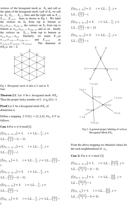
vertices of the hexagonal mesh as 𝑋0 and call as the spine of the hexagonal mesh. Left of 𝑋0 we call as 𝑋1, 𝑋2, … 𝑋𝑛−1 lines and the right side as 𝑋−1,

𝑋−2,…𝑋−𝑛+1 lines as shown in Fig 1. We label the vertices on 𝑋0 from top to bottom as

𝑣1,1, 𝑣1,2, … 𝑣1,2𝑛−1, the vertices on 𝑋1 from top to

bottom as 𝑣2,1, 𝑣2,2, … , 𝑣2,2𝑛−2, and so on , finally the vertices on 𝑋𝑛−1 from top to bottom as

𝑣𝑛,1, 𝑣𝑛,2, … 𝑣𝑛,𝑛. Similarly, we name 𝑋−1as

𝑣−1,1, 𝑣−1,2, … 𝑣−1,2𝑛−1,… and 𝑋−𝑛+1 as

𝑣−𝑛+1,1, 𝑣−𝑛+1,2, … 𝑣−𝑛+1,𝑛. The diameter of

𝐻𝑋𝑛is 2𝑛 − 2.

X

X

X X

X

0 -1

-2 1

2

Fig 1. Hexagonal mesh of dim n=3 and its X lines

Theorem 2.1

:

Let 𝐺 be a hexagonal mesh 𝐻𝑋𝑛.

Then the proper lucky number of 𝐺 is 𝜂𝑝 𝐺 = 3.

Proof.Let 𝐺 be a hexagonal mesh 𝐻𝑋𝑛 of

dimension 𝑛.

Define a mapping 𝑓: 𝑉(𝐺) → 1, 2,3 , ∀𝑣𝑖𝑗 ∈ 𝑉 as follows.

Case 1:For 𝑛 ≡ 0 𝑚𝑜𝑑(3)

𝑓 𝑣3𝑖−2, 3𝑗 −2 = 1. 𝑖 = 1,2, . . . 𝑛

3, 𝑗 =

1,2, … 2𝑛₃ − 𝑖 − 1 .

𝑓 𝑣3𝑖−1, 3𝑗 −1 = 1. 𝑖 = 1,2, . . .𝑛₃, 𝑗 =

1,2, … 2𝑛₃ − 𝑖.

𝑓 𝑣3𝑖, 3𝑗 = 1. 𝑖 = 1,2, . . . 𝑛

3, 𝑗 = 1,2, …

2𝑛 3 −

𝑖.

𝑓 𝑣3𝑖−2, 3𝑗 −1 = 3. 𝑖 = 1,2, . . .𝑛₃, 𝑗 =

1,2, … 2𝑛₃ − 𝑖 − 1 .

𝑓 𝑣3𝑖−1, 3𝑗 = 3. 𝑖 = 1,2, . . .𝑛₃, 𝑗 =

1,2, … 2𝑛₃ − 𝑖.

𝑓 𝑣3𝑖, 3𝑗 = 3. 𝑖 = 1,2, . . .𝑛₃, 𝑗 = 1,2, … 2𝑛₃ −

𝑖.

𝑓 𝑣3𝑖−2, 3𝑗 = 2. 𝑖 = 1,2, . . .𝑛₃, 𝑗 =

1,2, … 2𝑛₃ − 𝑖.

𝑓 𝑣3𝑖−1, 3𝑗 −2 = 2. 𝑖 = 1,2, . . .𝑛₃, 𝑗 =

1,2, … 2𝑛₃ − 𝑖 − 1 .

𝑓 𝑣3𝑖, 3𝑗 −1 = 2. 𝑖 = 1,2, . . .𝑛₃, 𝑗 =

1,2, … 2𝑛₃ − 𝑖.

1

2 3

2 3

1

2 3

1

3i-1,3j-1 v

3i-1,3j v

3i-2,3j v 3i-1,3j-2 v

3i,3j-2 v

3i-1,3j-2 v 3i,3j v

3i-1,3j-1 v

3i-1,3j v

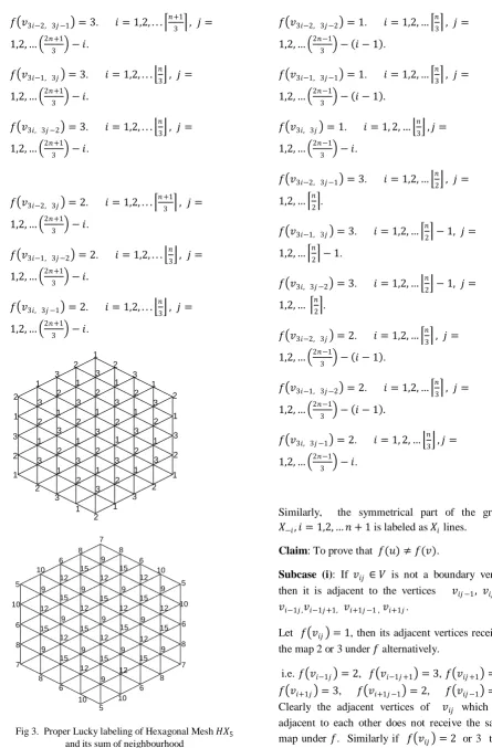
Fig 2. A general proper labeling of vertices in Hexagonal Mesh 𝐻𝑋𝑛

From the above mapping we obtained values for the each neighbourhood of 𝑣𝑖𝑗.

Case 2

: For

𝑛 ≡ 1 𝑚𝑜𝑑 (3)

𝑓 𝑣3𝑖−2, 3𝑗 −2 = 1. 𝑖 = 1,2, . . . 𝑛+1₃ , 𝑗 =

1,2, … 2𝑛+1₃ − 𝑖 − 1 .

𝑓 𝑣3𝑖−1, 3𝑗 −1 = 1. 𝑖 = 1,2, . . . 𝑛₃ , 𝑗 =

1,2, … 2𝑛+1₃ − 𝑖.

𝑓 𝑣3𝑖, 3𝑗 = 1. 𝑖 = 1,2, . . . 𝑛₃ , 𝑗 =

𝑓 𝑣3𝑖−2, 3𝑗 −1 = 3. 𝑖 = 1,2, . . . 𝑛+1

3 , 𝑗 =

1,2, … 2𝑛+1₃ − 𝑖.

𝑓 𝑣3𝑖−1, 3𝑗 = 3. 𝑖 = 1,2, . . . 𝑛

3 , 𝑗 =

1,2, … 2𝑛+1₃ − 𝑖.

𝑓 𝑣3𝑖, 3𝑗 −2 = 3. 𝑖 = 1,2, . . . 𝑛₃ , 𝑗 =

1,2, … 2𝑛+1₃ − 𝑖.

𝑓 𝑣3𝑖−2, 3𝑗 = 2. 𝑖 = 1,2, . . . 𝑛+1

3 , 𝑗 =

1,2, … 2𝑛+1₃ − 𝑖.

𝑓 𝑣3𝑖−1, 3𝑗 −2 = 2. 𝑖 = 1,2, . . . 𝑛₃ , 𝑗 =

1,2, … 2𝑛+1₃ − 𝑖.

𝑓 𝑣3𝑖, 3𝑗 −1 = 2. 𝑖 = 1,2, . . . 𝑛₃ , 𝑗 =

1,2, … 2𝑛+1₃ − 𝑖.

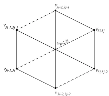
2 3 2 1 2 3 1 2 3 1 3 2 1 3 2 1 3 1 2 3 1 2 3 1 2 1 3 2 1 3 2 1 3 2 1 2 3 1 2 3 1 2 3 2 1 3 2 1 3 1 3 2 1 3 2 1 2 3 2 1 1 7 5 6 8 7 8 9 15 12 9 10 6 12 15 9 12 15 6 10 12 9 15 12 9 15 8 9 12 15 9 12 15 9 5 10 12 9 15 12 9 15 8 6 12 15 9 12 15 6 10 9 12 15 9 8 10 5 6 8 7 10

Fig 3. Proper Lucky labeling of Hexagonal Mesh 𝐻𝑋5

and its sum of neighbourhood

Case 3

:

For 𝑛 ≡ 2𝑚𝑜𝑑(3)

𝑓 𝑣3𝑖−2, 3𝑗 −2 = 1. 𝑖 = 1,2, … 𝑛

3 , 𝑗 =

1,2, … 2𝑛−1₃ − 𝑖 − 1 .

𝑓 𝑣3𝑖−1, 3𝑗 −1 = 1. 𝑖 = 1,2, … 𝑛

3 , 𝑗 =

1,2, … 2𝑛−1₃ − 𝑖 − 1 .

𝑓 𝑣3𝑖, 3𝑗 = 1. 𝑖 = 1, 2, … 𝑛₃ , 𝑗 =

1,2, … 2𝑛−1₃ − 𝑖.

𝑓 𝑣3𝑖−2, 3𝑗 −1 = 3. 𝑖 = 1,2, … 𝑛₂ , 𝑗 =

1,2, … 𝑛₂ .

𝑓 𝑣3𝑖−1, 3𝑗 = 3. 𝑖 = 1,2, … 𝑛₂ − 1, 𝑗 =

1,2, … 𝑛₂ − 1.

𝑓 𝑣3𝑖, 3𝑗 −2 = 3. 𝑖 = 1,2, … 𝑛₂ − 1, 𝑗 =

1,2, … 𝑛₂ .

𝑓 𝑣3𝑖−2, 3𝑗 = 2. 𝑖 = 1,2, … 𝑛

3 , 𝑗 =

1,2, … 2𝑛−1₃ − 𝑖 − 1 .

𝑓 𝑣3𝑖−1, 3𝑗 −2 = 2. 𝑖 = 1,2, … 𝑛

3 , 𝑗 =

1,2, … 2𝑛−1₃ − 𝑖 − 1 .

𝑓 𝑣3𝑖, 3𝑗 −1 = 2. 𝑖 = 1, 2, … 𝑛

3 , 𝑗 =

1,2, … 2𝑛−1₃ − 𝑖.

Similarly, the symmetrical part of the graph

𝑋−𝑖, 𝑖 = 1,2, … 𝑛 + 1 is labeled as 𝑋𝑖 lines.

Claim: To prove that 𝑓(𝑢) ≠ 𝑓(𝑣).

Subcase (i): If 𝑣𝑖𝑗 ∈ 𝑉 is not a boundary vertex

then it is adjacent to the vertices 𝑣𝑖𝑗 −1, 𝑣𝑖𝑗 +1,

𝑣𝑖−1𝑗 ,𝑣𝑖−1𝑗 +1, 𝑣𝑖+1𝑗 −1 , 𝑣𝑖+1𝑗.

Let 𝑓 𝑣𝑖𝑗 = 1, then its adjacent vertices receives the map 2 or 3 under 𝑓 alternatively.

i.e. 𝑓 𝑣𝑖−1𝑗 = 2, 𝑓 𝑣𝑖−1𝑗 +1 = 3, 𝑓 𝑣𝑖𝑗 +1 = 2,

𝑓 𝑣𝑖+1𝑗 = 3, 𝑓 𝑣𝑖+1𝑗 −1 = 2, 𝑓 𝑣𝑖𝑗 −1 = 3.

Subcase (ii): If 𝑣𝑖𝑗 ∈ 𝑉 is a boundary vertex then it is adjacent to the vertices 𝑣𝑖−1𝑗, 𝑣𝑖−1𝑗 +1, 𝑣𝑖𝑗 +1 or

𝑣𝑖−1𝑗 , 𝑣𝑖−1𝑗 +1, 𝑣𝑖𝑗 +1 .

Let 𝑓 𝑣𝑖𝑗 = 1, then its adjacent vertices receives

the map 2 or 3 under 𝑓 alternatively.

i.e. 𝑓 𝑣𝑖−1𝑗 = 2, 𝑓 𝑣𝑖−1𝑗 +1 = 3, 𝑓 𝑣𝑖𝑗 +1 = 2,

𝑓 𝑣𝑖+1𝑗 = 3 or 𝑓 𝑣𝑖−1𝑗 = 2, 𝑓 𝑣𝑖−1𝑗 = 2.

Clearly the adjacent vertices of 𝑣𝑖𝑗 which are adjacent to each other does not receive the same map under 𝑓. Similarly if 𝑓 𝑣𝑖𝑗 = 2 or 3 then

its

adjacent vertices receives the map 1 and 3 or 1 and 2 under 𝑓 alternatively as discussed above.

Clearly 𝑓(𝑢) ≠ 𝑓(𝑣), for all 𝑢, 𝑣 ∈ 𝐸 𝐺 . Hence the given labeling is a proper labeling.

Next we claim that the given mapping is a lucky labeling. That is, to prove 𝑠 𝑢 ≠ 𝑠 𝑣

for all (𝑢, 𝑣) ∈ 𝐸 𝐺 .

We obtain s 𝑣𝑖𝑗 , the inner sum of labels over all neighbours of vertex 𝑣𝑖𝑗 .

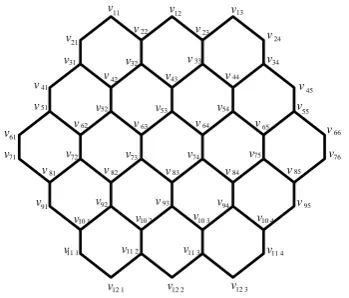
Consider any vertex of 𝐻𝑋𝑛. Let 𝑣(3𝑖, 3𝑗 ) be the

vertex with six adjacent vertices

say

𝑣

(3𝑖, 3𝑗 −1)

, 𝑣

(3𝑖−1, 3𝑗 )

, 𝑣

(3𝑖−1, 3𝑗 −2)

, 𝑣

(3𝑖, 3𝑗 −2)

,

𝑣

_{(3𝑖−2, 3𝑗 )}and

𝑣

_{(3𝑖−2, 3𝑗 −1)}

.

Fig 4.Sum of neighbourhood of

𝑣

_{(3𝑖, 3𝑗 )}

Fig 4.Sum of neighbourhood of

𝑣

_{(3𝑖, 3𝑗 )}

v_3i,3j v

3i,3j-1

3i,3j-2

3i-1,3j

3i-1,3j-2 3i-2,3j

3i-2,3j-1

v

v

v

v

v

Fig 4. Sum of neighbourhood of 𝑣(3𝑖, 3𝑗 )

Hence its sum of neighbourhood are

𝑠 𝑣3𝑖, 3𝑗 = 𝑓 𝑣3𝑖, 3𝑗 −1 + 𝑓 𝑣3𝑖−1, 3𝑗

+ 𝑓 𝑣3𝑖−1, 3𝑗 −2 + 𝑓 𝑣3𝑖, 3𝑗 −2

+ 𝑓 𝑣3𝑖−2, 3𝑗 + 𝑓 𝑣3𝑖−2, 3𝑗 −1

= 2+3+2+3+2+3

= 15

Here we are taking 𝑣(3𝑖−2, 3𝑗 ) the adjacent vertices

of 𝑣3𝑖, 3𝑗 .

v3i-2,3 j v_3i-2,3j-1

3i-2,3j-2

3i,3j

3i,3j-2 3i-1,3j

3i-1,3j-1 v

v

v

v

v

Fig 5. Sum of neighbourhood of 𝑣(3𝑖−2, 3𝑗 )

𝑠 𝑣3𝑖−2, 3𝑗 = 𝑓 𝑣3𝑖−2, 3𝑗 −1 + 𝑓 𝑣3𝑖, 3𝑗

+ 𝑓 𝑣3𝑖, 3𝑗 −2 + 𝑓 𝑣3𝑖−2, 3𝑗 −2

+ 𝑓 𝑣3𝑖−1, 3𝑗 + 𝑓 𝑣3𝑖−1, 3𝑗 −1

= 3+1+3+1+3+1

= 12

v_3i,3j-2 v_3i,3j

3i,3j-1

3i-1,3j-2

3i-1,3j-1 3i-2,3j-2

3i-2,3j

v

v

v

v

v

Fig 6. Sum of neighbourhood of 𝑣(3𝑖, 3𝑗 −2)

Similarly, we can show that 𝑠 𝑣3𝑖, 3𝑗 −2 = 9,

𝑠 𝑣3𝑖−2, 3𝑗 −1 = 9,

𝑠 𝑣3𝑖, 3𝑗 −1 = 12 , 𝑠 𝑣3𝑖−1, 3𝑗 = 9 ,

From the above cases we see that 𝑠 𝑢 ≠ 𝑠 𝑣 for

all 𝑢𝑣 ∈ 𝐸 𝐺 .

Similarly, we can prove other cases.

Therefore 𝜂𝑝 ≤ 3 .

Since the clique number of 𝐻𝑋𝑛 is 3, and by the theorem 1.2 𝜂𝑝≥ 3. Therefore 𝜂𝑝 𝐺 = 3.

3. Proper Lucky Number of Honeycomb

Networks

A high level honeycomb network can be constructed from a low level one. A unit honeycomb network is a hexagon, denoted by HC(1). Honeycomb network of size 2 denoted HC(2), can be obtained by adding six hexagons around the boundary edges of HC(1). Inductively, honeycomb network HC(n) can be obtained from HC(n – 1) by adding a layer of hexagons around the boundary edges of HC(n – 1). Alternatively, the size d of HC(n) is determined as the number of hexagons between the center and boundary of HC(n) (inclusive) and the number of vertices and edges of HC(n) are 6𝑛2 and 9𝑛2− 3𝑛 respectively. We use the level numbering scheme proposed by the Sharieh et al.[14] for the honeycomb networks. Each node in HC(n) is identified by a 𝑣𝑖𝑗, where

idenotes the line number in which the node exists, and j denotes the location of the node in the line. A node with the address 1,1 is the first node that exists at line number 1. The node 1,2 refers to the second node that exists at line number 1, and so on. See Fig 7.

v v v

v v v v

v v v v v

v v v v v v

v v v v v

v v v v

v v v v

v v v

v v

v v v v v v

v v v v

v

v v v

v v v

v

11 12 13

21

22 23

24

31 32 33 34

41

42 43 44

45

51 52 53 54 55

61

62 63 64 65

66

71 72 73 74 75 76

81 82 83 84 85

91 92 93 94 95

10 1 10 2 10 3 10 4

11 1 11 2 11 3 11 4

12 1 12 2 12 3

Fig 7. Honeycomb network with addressing HC(3)

Theorem 3.1: Let 𝐺 be a honeycomb 𝐻𝐶 𝑛 .

Then the proper lucky number of 𝐺 is 𝜂𝑝 𝐺 = 2.

Proof. Let 𝐺 be a honeycomb graph 𝐻𝐶 𝑛 of

dimension 𝑛.

Define a mapping 𝑓: 𝑉(𝐺) → 1, 2 , ∀𝑣𝑖𝑗 ∈ 𝑉 as follows

𝑓 𝑣𝑖𝑗 = 1, 𝑖 𝑖𝑠 𝑜𝑑𝑑_{2, 𝑖 𝑖𝑠 𝑒𝑣𝑒𝑛}

Subcase (i): If 𝑣𝑖𝑗 ∈ 𝑉 is not a boundary vertex

then it is adjacent to the even line vertices 𝑣𝑖−1𝑗 −1,

𝑣𝑖−1𝑗, 𝑣𝑖+1 𝑗 , upto 2𝑛 lines and it is adjacent to

the odd line vertices 𝑣𝑖−1𝑗, 𝑣𝑖+1 𝑗, 𝑣𝑖+1 𝑗 +1 , upto

2𝑛 − 1. Below the line 2𝑛, 𝑣𝑖𝑗 is adjacent to even

line vertices 𝑣𝑖−1𝑗, 𝑣𝑖−1 𝑗 +1, 𝑣𝑖+1𝑗 upto 4𝑛-2 and it is adjacent to the odd line vertices 𝑣𝑖−1𝑗,

𝑣𝑖+1𝑗 −1, 𝑣𝑖+1 𝑗 upto 2𝑛 − 1.

Let 𝑓 𝑣𝑖𝑗 = 1, then its adjacent vertices receives the map 2 under 𝑓 alternatively.

Clearly the adjacent vertices of 𝑣𝑖𝑗 which are adjacent to each other does not receive the same map under 𝑓. Similarly if 𝑓 𝑣𝑖𝑗 = 2 then its adjacent vertices receives the map 1 under

𝑓 alternatively.

Subcase (ii): If 𝑣𝑖𝑗 ∈ 𝑉 is a boundary vertex then

the first line of 𝐻𝐶(𝑛) is adjacent to the vertices

𝑣𝑖+1𝑗, 𝑣𝑖+1 𝑗 +1 and the 𝑛𝑡ℎ line is adjacent to the vertices 𝑣𝑖−1𝑗, 𝑣𝑖−1 𝑗 +1 . The left side of the boundary is adjacent to the vertices 𝑣𝑖−1𝑗, 𝑣𝑖+1 𝑗 and the right side of 𝑣𝑖𝑗 is adjacent to even line vertices 𝑣𝑖−1 𝑗 −1, 𝑣𝑖+1𝑗 and the odd line vertices 𝑣𝑖−1𝑗, 𝑣𝑖+1𝑗 +1 upto 2𝑛 lines and below the 2𝑛 lines 𝑣𝑖𝑗 is adjacent to even line vertices

𝑣𝑖−1 𝑗 +1, 𝑣𝑖+1𝑗 and the odd line vertices

𝑣𝑖−1𝑗, 𝑣𝑖+1𝑗 −1.

Let 𝑓 𝑣𝑖𝑗 = 1, then its adjacent vertices receives

the map 2 under 𝑓 alternatively.

Clearly the adjacent vertices of 𝑣𝑖𝑗 which are adjacent to each other does not receive the same map under𝑓. Similarly if 𝑓 𝑣𝑖𝑗 = 2 then its adjacent vertices receives the map 1 under

1 1 1

2 2 2 2

1 1 1 1

2 2 2 2 2

1 1 1 1 1

2 2 2 2 2 2

1 1 1 1 1 1

2 2 2 2 2

1 1 1 1 1

1 1 1 1

2 2 2 2

2 2 2

4 4 4

2 3 3 2

6 6 6 6

2 3 3 3 2

6 6 6 6 6

2 3 3 3 3 2

4 6 6 6 6 4

3 3 3 3 3

4 6 6 6 4

4 6 6 4

2 2 2 2

2 2 2

Fig 8. Proper Lucky labeling of Honeycomb 𝐻𝐶 3 and its sum of neighbourhood

Proof is similar to theorem 2.1.

Conclusion:

In this paper, we obtained the proper lucky number for Hexagonal mesh and Honeycomb network. Futher, we investigate the problems in various interconnection networks such as butterfly, benes, torus etc.

Reference :

1. L. Addhario- Berry, R.E.L.Aldred, K.Dalai, B.A. Reed,

“Vertex coloring edge partitions”, Journal of combinatorial Theory series, vol 94 n.2, p 237-244, July 2005.

2. A. Ahai, A. Dehghan, M. Kazemi, E. Mollaahmedi,

“Computation of Lucky number of planar graphs is NP-hard”, Information processing letters, vol 112, Iss 4, p 109-112, 15th _{Feb 2012.}

3. S. Akhari, M. Ghanbari, R. Manariyat, S. Zare, „ On the lucky choice number of graphs”, Graphs and combinatorics, vol 29 n.2, p 157-163, Mar 2013.

4. G. Chartand, F.Okamoto, P.Zhang, “The sigma chromatic

number of a graph”, Graphs and combinatorics 26 (6), p 755- 773, 2010.

5. Czerwinski, Sebastian, Grytczuk, Jaroslaw, Elazny and

Wiktor, “ Luckylabeling of graphs”, Inf. Process. Lett. 109(18); 1078-1081. Zbl 1197.05125, 2009.

6. A. Dehghan, M.R. Sadeghi, A. Ahadi, “ Algorithmic

complexity of proper labeling problems”, Theoretical computer science, vol 495, p 25-36, 2013.

7. J.Gallian, “ A Dynamic survey of graph labeling,” The

Electronic journal of combinatorics, 1996- 2005.

8. Y.Kins, R.C. Thivyarathi, D.Antony Xavier, “ Proper

Lucky number of Mesh derived aricheture”,

9. LeenaSankari S., Masthan K.M.K., AravindhaBabu N.,

Bhattacharjee T., Elumalai M., "Apoptosis in cancer - an

update", Asian Pacific Journal of Cancer Prevention, ISSN : 1513-7368, 13(10) (2012) PP. 4873-4878.

10. Michal Karonski, Tomasz Luczak, Andrew Thomason,

“Edge weights and vertex colors”, Journal of combinatorics theory series B, vol 91n.1, p151-157, May 2004.

11. A. NellaiMurugan, R. Maria Irudhaya Aspin Chitra,

“Lucky Edge Labeling of Pn, Cn and Corona of Pn, Cn”, IJSIMR, Volume 2, Issue 8, August 2014, pp. 710-718

12. S. Ramachandran and S.Arumugam, „Invitation to graph

theory‟, Scitech publication pvt.Ltd, Reprint, Jan 2009.

13. Subhashree A.R., Parameaswari P.J., Shanthi B., Revathy

C., Parijatham B.O., "The reference intervals for the haematological parameters in healthy adult population of Chennai, Southern India", Journal of Clinical and Diagnostic Research, ISSN : 0973 - 709X, 6(10) (2012), PP. 1675-1680.

14. Sharieh A, Qatawneh M, Almobaideen W, Sleit A,