The Thirty-Third AAAI Conference on Artificial Intelligence (AAAI-19)
Fast Incremental SVDD Learning Algorithm with the Gaussian Kernel
Hansi Jiang, Haoyu Wang, Wenhao Hu, Deovrat Kakde, Arin Chaudhuri
SAS Institute Inc.100 SAS Campus Drive Cary, North Carolina 27513
{Hansi.Jiang; Haoyu.Wang; Wenhao.Hu; Dev.Kakde; Arin.Chaudhuri}@sas.com
Abstract
Support vector data description (SVDD) is a machine learn-ing technique that is used for slearn-ingle-class classification and outlier detection. The idea of SVDD is to find a set of sup-port vectors that defines a boundary around data. When deal-ing with online or large data, existdeal-ing batch SVDD methods have to be rerun in each iteration. We propose an incremen-tal learning algorithm for SVDD that uses the Gaussian ker-nel. This algorithm builds on the observation that all support vectors on the boundary have the same distance to the center of sphere in a higher-dimensional feature space as mapped by the Gaussian kernel function. Each iteration involves only the existing support vectors and the new data point. More-over, the algorithm is based solely on matrix manipulations; the support vectors and their corresponding Lagrange multi-plierαi’s are automatically selected and determined in each
iteration. It can be seen that the complexity of our algorithm in each iteration is onlyO(k2), wherek is the number of support vectors. Experimental results on some real data sets indicate that FISVDD demonstrates significant gains in effi-ciency with almost no loss in either outlier detection accuracy or objective function value.
1
Introduction
Much effort has been made to detect faults and state shifts in industrial machines through monitoring data sensors. Suc-cessful fault diagnosis reduces cost of maintenance and improves both worker and machine efficiency. In machine learning, fault diagnosis can be viewed as an outlier de-tection problem. Support vector data description (SVDD), a machine learning technique that is used for single-class classification and outlier detection, is similar to support vec-tor machine (SVM). SVDD was first introduced in Tax and Duin (2004), although the concept of using SVM to detect novelty was introduced in Sch¨olkopf et al. (2000). SVDD is used in domains where the majority of data belongs to a sin-gle class, or when one of the classes is significantly under-sampled. The SVDD algorithm builds a flexible boundary around the target class data; this data boundary is character-ized by observations that are designated as support vectors. Having the advantage that no assumptions about the distri-bution of outliers need to be made, SVDD can describe the
Copyright c2019, Association for the Advancement of Artificial Intelligence (www.aaai.org). All rights reserved.
shape of the target class without prior knowledge of the spe-cific data distribution and can flag observations that fall out-side the data boundary as potential outliers. In the case of machine monitoring, data on the normal working conditions of a machine are in abundance, whereas information from outlier system failures are few. By using SVDD on the well-sampled target class, one can obtain a boundary around the distribution of normal working data, and subsequently cap-ture the outlier points where the machine is faulty.
Traditional batch methods of SVDD typically pursue a global optimal solution of the SVDD problem; they suffer from low efficiency by considering all available data points. Moreover, these methods are usually ineffective when han-dling streaming data because the entire algorithm must be re-run with each incoming data point. In contrast, incremental methods deal with large or streaming data efficiently by fo-cusing on smaller portions of the original optimization prob-lem, as in Syed et al. (1999). Online variants of SVDD con-centrate only on the current support vector set with incoming data.
Cauwenberghs and Poggio (2001) give an incremental and decremental training algorithm for SVM. Their method, also called the C&P algorithm, provides an exact solution for training data and one new data point. Tax and Laskov (2003) use a numerical method to solve incremental SVM, and they describe the relationship between incremental SVM and on-line SVDD. Their research was extended in Laskov et al. (2006), which provides complete learning algorithms for in-cremental SVM and SVDD.
The algorithm given in Laskov et al. (2006) updates weights of each support vector based on the fact that Karush-Kuhn-Tucker (KKT) conditions must be satisfied before and after a new data point comes in. Consequently, all data points must be kept to pursue an objective value closer to the global optimal value. Furthermore, a kernel matrix must be calcu-lated every update, which can be memory-consuming and slow for large data.
Unlike the method in Laskov et al. (2006), FISVDD uses only matrix manipulations to find interior points and sup-port vectors, and it is highly efficient in detecting outliers. It can be used either as a batch method or as an online method. It can be seen that the complexity of key parts of FISVDD is O(k2), wherekis the number of support vectors. By Kakde et al. (2017), the number of support vectors should be much less than the number of observations in order to avoid over-fitting.
The rest of the paper is organized as follows. In Section 2, we introduce the SVDD problem in Tax and Duin (2004). In Section 3, we state some theoretical support for FISVDD. In Section 4, the FISVDD algorithm is introduced and ex-plained. In Section 5, we discuss several important issues in implementing FISVDD. In Section 6, FISVDD is applied to some data sets and compared with other methods. Finally, in Section 7, we give our conclusions.
In this paper we follow traditional linear algebra notation. Bold capital letters stand for matrices, and bold small letters stand for vectors. Specifically, matrixAis used as a Gaus-sian kernel matrix, andAkis the Gaussian kernel matrix in
thekth iteration. The vectorx>0stands for a positive vec-tor, andx≥0stands for a nonnegative vector.
2
The SVDD Problem
The SVDD problem is first discussed by Tax and Duin (2004). The idea of SVDD is to find support vectors and use them to define a boundary around data. If a testing data point lies outside the boundary, it is classified as an outlier; other-wise, it is classified as normal data. The simplest form of a boundary is a sphere. For a set of data pointsx1,x2, . . . ,xn,
the mathematical formulation of the problem is to find a nonnegative vectorαthat contains Lagrange multipliers for all data points,kαk1 = 1, such that the following is
maxi-mized:
L= n
X
i=1
αihxi,xii −
X
i,j
αiαjhxi,xji. (2.1)
Herehxi,xjiis the inner product ofxi andxj. According
to Tax and Duin (2004), there are three possibilities for each data point. Thexi’s that have zeroαi’s areinterior points.
Thexi’s for which0< αi< Cfor a preselected0< C ≤1
lie on the boundary and are calledsupport vectors. Thexi’s
for whichαi =Care outliers (also calledbounded support
vectors, or bsv, in Ben-Hur et al. (2001)). In this paper, we
assume there are no outliers in the training phase, so we set C= 1. One example of where our algorithm would be use-ful is when there is a known period during which the incom-ing data are normal, such as streamincom-ing sensor data from ma-chines or vehicles operating under normal conditions. Then the model can be used to detect abnormal states. To deter-mine whether a new data point zlies inside the boundary, first the distance betweenzand the center of the sphere,a, is calculated:
d2(z) =kz−ak2=hz,zi
−2X i
αihz,xii+
X
i,j
αiαjhxi,xji. (2.2)
This distance is then compared to the radius of the sphere for any support vectorxk:
R2=hxk,xki
−2X i
αihxk,xii+
X
i,j
αiαjhxi,xji. (2.3)
A test data pointzis accepted ifd2≤R2, and it is classified
as an outlier ifd2 > R2. This check is also calledscoring. It is easy to derive the conclusion that scoring is equivalent to checking whether the new data point violates the current KKT conditions.
A kernel function is needed to draw a more flexible boundary around data in order to avoid underfitting. By Tax and Duin (2004), using a kernel function is equivalent to im-plicitly mapping data points to a higher feature space. Usu-ally the Gaussian kernel,
K(xi,xj) = exp(−
kxi−xjk22
2σ2 ), (2.4)
is preferred (Ben-Hur et al. 2001; Laskov et al. 2006; Gu et al. 2015), and the Gaussian kernel bandwidthσmust be selected beforehand. There are some papers that discuss how to choose a proper Gaussian kernel bandwidth (Evan-gelista, Embrechts, and Szymanski 2007; Xiao et al. 2014; Kakde et al. 2017). Throughout this paper, it is assumed that the Gaussian similarity is used and that a proper Gaussian kernel bandwidth σhas been chosen such that the number of support vectors is much less than the number of observa-tions. As stated in Section 5, FISVDD has protections even if a bad bandwidth is provided. With the Gaussian kernel function, the objective function Eq. 2.1 can be simplified to minimizing
L=X i,j
αiαjK(xi,xj), (2.5)
becauseK(xi,xi) = 1,kαk1= 1, andαis nonnegative.
Eq. 2.5 can also be expressed in matrix form:
L=αTAα, (2.6)
whereAis a Gaussian similarity matrix for all support vec-tors andα >0. Formulas Eq. 2.2 and Eq. 2.3 then become as follows, respectively:
d2(z) = 1−2X i
αiK(z,xi) +
X
i,j
αiαjK(xi,xj), (2.7)
R2= 1−2X i
αiK(xk,xi) +
X
i,j
αiαjK(xi,xj). (2.8)
Note that to determine whether a test data pointzshould be accepted, one can compute only
Q(z) = (d2(z)−R2)/2 =
X
i
αiK(xk,xi)−
X
i
αiK(z,xi). (2.9)
Q(z)≤0means thatzis an interior point. It is worth men-tioning that all support vectors satisfyd2 = R2, although
3
Theoretical Foundations
Here we state and prove several theorems necessary for later discussion. First, we state a lemma in Smola and Sch¨olkopf (1998) that a Gaussian similarity matrix has full rank. A di-rect conclusion of the lemma is that a Gaussian similarity matrix is symmetric positive definite (spd).
Lemma 1. Supposex1,x2, . . . ,xk are distinct points and
σ6= 0. Then their Gaussian similarity matrixAformed with
Eq. 2.4 has full rank.
Lemma 1 implies thatAis spd and its inverse exists. Next, we state lemmas to obtainA−k+11 ifA−k1is known and vice versa. In FISVDD, we need to update the inverse of the sim-ilarity matrix when a new data point comes in. The proof involves only matrix calculations and is skipped.
Lemma 2. SupposeAkandAk+1are both Gaussian
simi-larity matrices and
Ak+1=
Ak v
vT 1
. (3.1)
IfA−k1is known, thenA−k+11 is given by
A−k+11 =
A−k1+ppT/β −p/β
−pT/β 1/β
, (3.2)
wherep=A−k1vandβ = 1−vTA−k1v= 1−vTp.
Lemma 2 provides a method to compute A−k+11 by us-ingA−k1and an incremental vectorv. Note that to compute A−k+11 , we only need to computep=A−k1v. Also note that βis the Schur complement (Meyer 2000) ofA−k1inA−k+11 . SinceAk+1is spd,βis positive (Gallier 2010). The inverse
of Lemma 2 is straightforward and shown below.
Lemma 3. SupposeAk+1is spd and its inverse is given by
A−k+11 =
Pk×k u
uT λ
. (3.3)
Then the inverse ofAkis
A−k1=P−uuT/λ. (3.4) Lemma 2 and Lemma 3 together play an essential role in FISVDD to increase efficiency. It can be seen from the lemmas that onlyO(k2)multiplications are needed to obtain
the updated matrix inverse. Next, we prove that if a positive solution is obtained for the linear systemAα=e, then all data points in the system are support vectors. This is from the property that all support vectors satisfyd2=R2.
Theorem 4. A set of data pointsx1,x2, . . . ,xkare all
sup-port vectors if and only if
Akα=e (3.5)
has a positive solution, whereeindicates a vector that
con-tains all 1’s with proper dimension.
Proof. Suppose thatx1,x2, . . . ,xk are all support vectors.
Then they all satisfyd2(x
i) = R2in Eq. 2.9, and thus the
d2(x
i)’s are all equal. From Eq. 2.7, the middle terms,
X
i
αiK(z,xi), (3.6)
are all equal for any support vector z. Putting Eq. 3.6 to-gether for all support vectors results in the left-hand side of Eq. 3.5. Therefore, Eq. 3.5 has a positive solution. On the other hand, Eq. 3.5 implies that allxi’s satisfyd2(xi) =R2
and thus are all support vectors.
If a new data pointxk+1is added to the existing support
vector set but the (k+ 1)th position in the solution to the linear systemAk+1α=eis not positive, then the new data
point is an interior point. This is proven in the next theorem. Theorem 5. Suppose data pointsx1,x2, . . . ,xkform a
sup-port vector set. Then a new data pointxk+1 is an interior
point if and only ifAk+1α=e⇒αk+1 ≤0.
Proof. Suppose that Ak+1α = e ⇒ αk+1 ≤ 0. By
Lemma 2, we have
αk+1= [A−k+11 e]k+1=
−pT/β 1/βe. (3.7)
Becauseαk+1≤0, we have
αk+1=
1−eTA−k1v
1−vTA−1
k v
≤0. (3.8)
Becauseβ= 1−vTA−1
k v>0, we have
1−eTA−k1v≤0. (3.9)
We want to prove thatd2−R2≤0forxk+1. Note that
(d2−R2)/2 =αkTAk(∗i)−αTkv = (A−k1e)TAk(∗i)−(A−
1
k e) Tv
=eTA−k1Ak(∗i)−e
TA−1
k v = 1−eTA−k1v,
(3.10)
whereAk(∗i)is theith column ofAk. By Eq. 3.9, we have
d2−R2≤0.
On the other hand, suppose xk+1 is strictly inside the
boundary. Then we have
(d2−R2)/2 = 1−eTA−k1v≤0. (3.11) Then
αk+1=
1−eTA−1
k v 1−vT
kA
−1
k v
≤0. (3.12)
Theorem 5 says that if we put a new data pointxi into
an existing support vector set to form an expanded set and the(k+ 1)th position in the solution to the expanded system Ak+1α =eis less than 0, thenxiis an interior point and
thus can be ignored. Because we can permute the rows and columns inA−k+11 , by Theorem 5 ifαi ≤0for1≤i≤k, we
can takexiout of the expanded set and solve the shrunken
k×klinear system. We can continue shrinking the system until there are no negative entries inα; then a support vector set is obtained. We summarize this shrinking step in the next corollary.
Corollary 6. A data pointxiis an interior point if and only
ifAk+1α =e ⇒ αi ≤ 0and the shrunkenk×klinear
Finally, we state and prove an observation that relates the objective function value, the 1-norm of theunnormalizedα
vector, and the scoring threshold. The observation is sub-stantial for implementing FISVDD. With it a lot of unnec-essary computations can be saved. This observation can be also used to make sure that the objective function value in FISVDD is not larger than the objective function value ob-tained in the previous iteration so the FISVDD model is im-proved.
Corollary 7. The objective function value in Eq. 2.6 with
positiveα,kαk1= 1, satisfies
L= 1
kα0k1
, (3.13)
whereα=α0/kα0k1. Moreover, it holds that
L=X i
αiK(z,xi), (3.14)
where thexi’s are the support vectors andzis any one of
the support vectors.
Proof. To prove Eq. 3.13, note that by Theorem 4,α0
satis-fiesAα0=e. Then
L=αTAα= α T
0
kα0k1
A α0 kα0k1
= α
T
0e
kα0k21
= kα0k1
kα0k21
= 1
kα0k1
.
(3.15)
To prove Eq. 3.14, note thatP
iαiK(z,xi)is the first term
of the right-hand side of Eq. 2.9. So proving Eq. 3.14 is equivalent to proving
X
i,j
αiαjK(xi,xj) =
X
i
αiK(z,xi), (3.16)
wherexi,xj are support vectors, andzis any one of the
support vectors. The following equation can be derived:
X
i,j
αiαjK(xi,xj) =
X
j
αj
X
i
αiK(xi,xj)
= X
i
αiK(z,xi)
X
j
αj
=X
i
αiK(z,xi).
(3.17)
The second equality is derived from the fact that the term in parentheses is a constant for any support vectorxj, and the
third equality is derived from the fact that the sum of allαi’s
is 1.
Corollary 7 shows a direct relationship between the objec-tive function value, the 1-norm of the solution vector to the linear systemAα =e, and the scoring threshold. The ob-jective function value is a very important term of an SVDD model and can be requested by the user at any time. When the solution vector of the linear system is derived, the inverse of its 1-norm directly gives the objective function value, and
the calculations in Eq. 2.6 are avoided. At the same time,L is also the scoring threshold for the current model. Only the second term in Eq. 2.9 needs to be computed when a new data point needs to be scored. The results from Corollary 7 help make our FISVDD algorithm more efficient.
4
Fast Incremental SVDD Learning
Algorithm
We propose a fast incremental algorithm of SVDD (FISVDD). The central idea of FISVDD is to minimize the objective function (2.6) by quickly updating the inverse of similarity matrices in each iteration. Suppose that we be-gin with a support vector setx1,x2, . . . ,xk. When a new
data pointxk+1comes in, by Theorem 4 the linear system
Ak+1α =ewill have a positive solution if thek+ 1data
points form a new support vector set, and the normalizedα
vector gives theαi’s. However, if at least one of the entries
in the solution is negative, that indicates there is at least one interior point in the set. Then we are able to drop the nega-tiveαithat has the largest|d2−R2|magnitude and solve the
shrunkenk×klinear system. If the system has a positive so-lution, then we have found a support vector set. Otherwise, we can continue to drop the next negativeαi that has the
largest|d2−R2|magnitude and solve the(k−1)×(k−1)
lin-ear system, and so on. It is worth noting that if more than one variable is dropped from the system, the dropped data points should be re-scored against the new boundary to determine whether the KKT conditions are violated. If the KKT con-ditions are violated, then the system will expand again. We provide details below.
The FISVDD Algorithm
The FISVDD algorithm is shown in Algorithm 3. It contains three parts of FISVDD: expanding (which is shown in Al-gorithm 1), shrinking (which is shown in AlAl-gorithm 2), and bookkeeping.
Stage 1, Expanding When a new data pointxk+1comes
in, it is scored to determine whether it falls in the interior. If so, it is immediately discarded. Otherwise, it is combined with existing support vectors to form an expanded set. The corresponding inverse matrix of the similarity matrix and its row sums are then updated by Lemma 2. If all row sums are positive, thenxk+1 is another support vector and the
nor-malized αvector contains the updatedαi’s. Ifαk+1 ≤ 0,
thenxk+1 is taken out of the expanded set and the support
vector set returns to the previous set. Ifαk+1 >0but there
is at least oneαi≤0, then there is at least one interior point
in the expanded set and the shrinking step is called. The ex-panding step is given in Algorithm 1.
Stage 2, Shrinking Ifαk+1 >0but at least oneαi <0,
then at least one existing support vector in the support vec-tor set has become an interior point. We need to identify and discard such vectors. By Corollary 6, we can shrink the support vector set one vector at a time until a positive α
Algorithm 1Expand
1: Input:xk+1,α,SV, σ,A−1
2: v←K(xk+1,SV, σ)
3: A−old1←A−1
4: A−1←Eq. 3.2
5: αold←α
6: α←row sums ofA−1
7: ifαk+1≤0then
8: A−1←A−1 old
9: α←αold
10: else
11: SV←SV +xk+1
12: end if
13: Return:α,SV,A−1
take out one vector at a time rather than taking out several vectors. Moreover, taking out several vectors at once slows the algorithm because then we need to calculate the inverse of matrices whose rank is larger than 1. Although there is no certain way of choosing which vector to remove first, in FISVDD we choose the negativeαithat has the largest
mag-nitude. From Eq. 3.8 and Eq. 3.10 and permuting columns and rows inAk+1, we have
αk+1=
d2−R2
2(1−vTA−1
k v)
, (4.1)
whereαk+1is theαiof interest permuted to the(k+1)th
po-sition. It can be seen from Eq. 4.1 that if the denominators of the data points that have negativeαi’s are close, then a data
point that has a larger|αi|tends to have a larger|d2−R2|,
which means it lies farther from the boundary. Intuitively, a data point farther from the boundary is more likely to be a true interior point. Although not guaranteed, the data point farthest from the boundary is typically the one we want to remove first.
Algorithm 2Shrink
1: Input:α,SV,A−1,Backup
2: flag←1
3: whileflag = 1do 4: p←arg minα
5: Backup←Backup +xp
6: SV←SV−xp
7: A−1←Eq. 3.4
8: α←row sums ofA−1
9: ifminα>0then 10: flag←0
11: end if 12: end while
13: Returnα,SV,A−1,Backup
Bookkeeping When the shrinking algorithm is performed, some of the previous support vectors are taken out of the support vector set if they have negativeαi’s. However,
hav-ing a negativeαi in the middle of a shrinking process does
not rule a support vector out from the final set. A data point is considered to be an interior point only if it satisfies
(d2−R2)<0when scored with the final support vector set.
Therefore, it is necessary to recheck whether the data points taken out of the support vector set are truly interior points. In FISVDD, we build a backup set when the shrinking stage begins. When a data point is taken out of the support vector set, it is put into the backup set. Then the inverse matrix is “downdated” with Eq. 3.4 and its row sums are calculated. The shrinking continues until there are no negative entries in theαvector. The backup set keeps growing as the linear system shrinks. When there are no negative values inα, we have found a support vector set, although it might not be the final one. Then the data points in the backup set are scored with the support vector set one by one in a first in, first out order. To increase the algorithm’s efficiency, the backup set is scanned only once. If(d2−R2)>0for a data point, then the expanding algorithm is called again, and the data point is removed from the backup set and placed back into the sup-port vector set. The expanding finishes when all data points in the backup set have(d2−R2)≤ 0. Although the same
check can be performed on all prior data, doing so would cost too much memory and the gains are far less significant. So the backup set is emptied when each new data point ar-rives.
For completeness, we add a check to the unnormalizedα
vector to make sure that the result in each iteration is im-proved from the previous iteration. By Corollary 7, the re-sult is improved if the 1-norm of the unnormalizedαvector increases. At the end of each iteration, this norm is com-pared with the norm in the previous iteration. If the norm decreases, then the result from the previous iteration is re-stored. None of our experiments have ever violated this con-dition.
To summarize, FISVDD is fast and computationally ef-ficient because the algorithm ignores interior points and is built solely on matrix manipulations. First, FISVDD tries to obtain the optimal solution in each iteration without using the interior points, similar to the idea mentioned in Syed et al. (1999). Results from many experiments show that if a proper Gaussian bandwidth is chosen, then the number of support vectors should be far smaller than the total num-ber of observations. FISVDD takes advantage of this fact by calculating only the similarities between the new data points and the support vectors.
Secondly, it can be seen from Algorithm 3 that FISVDD is based only on matrix manipulation. Matrix inverse updating steps are the core of FISVDD, which lets the system itself choose which data points to move between support vector sets and interior point sets. Sometimes the choice of the sys-tem might not be optimal, but the existence of backup sets allows the system to correct itself and removes a significant number of calculations.
5
Implementation Details
Algorithm 3Fast Incremental Support Vector Data Descrip-tion (FISVDD)
1: Input:Initialize(α,SV,A−1, σ)
2: fori←1, ndo 3: Q←Eq. 2.9 4: ifQ≤0then 5: pass 6: else
7: α,SV,A−1←Expand(xk+1,α,SV, σ,A−1)
8: ifminα<0then
9: Backup←Empty set
10: α,SV,A−1,Backup
←Shrink(α,SV,A−1,Backup)
11: ifcard(Backup)>1then
12: forj←1,card(Backup)do
13: Q←Eq. 2.9
14: ifQ >0then 15: α,SV,A−1
←Expand(Backupj,α,SV, σ,A−1)
16: end if
17: end for
18: end if 19: end if 20: α←α/kαk1
21: end if 22: end for
Initialization
A key advantage of FISVDD is that the similarity matrixA is directly calculated only at initialization. As stated in Sec-tion 4, each iteraSec-tion calculates only the similarities between a new data point and the existing support vectors. These are used to update the inverse of the similarity matrix; the sim-ilarity matrix is calculated only at initialization. Once the burn-in data points are selected, their similarity matrix A and its inverse A−1 are calculated. After the row sums of
A−1are calculated, the shrinking step in Algorithm 2 is used
to pick out the interior points. Then the vector that contains the normalized row sums ofA−1is the initialα.
Memory
For any online method, it is important to make sure that both of the following conditions hold:
• The complexity in each step is small.
• Memory usage will never expand out of control even for very large data.
For FISVDD, the two challenges are handled smoothly. The first part is easy to see: The key parts in the algorithm (expanding and shrinking the linear systems) require only O(k2)multiplications each time, wherekis the number of
support vectors. In addition,kshould be far less than the to-tal number of the whole data set if a proper Gaussian kernel bandwidthσis chosen.
For the second part, the number of support vectors can in-deed grow large with streaming data. To avoid the potential
threat of memory expanding out of control, we set a param-eter,M, for the maximal number of support vectors, where M depends on availability of memory. WhenM is reached, the number of support vectors will not grow large. If a new data point xk+1 satisfies d2 > R2, then one of the three
situations will occur:
• αk+1 >0but at least one of theαi’s is less than or equal
to 0. In this case, the algorithm runs normally to select the interior points.
• Allαi’s are greater than 0, butαk+1is the smallest among
allαi’s. In this case,αk+1is discarded.
• Allαi’s are greater than 0, andαk+1is not the smallest
among allαi’s. In this case, the support vector that has
the smallestαiis replaced byxk+1, and the newαi’s are
updated.
By handling these three cases, the number of support vec-tors will not exceedM, and the memory usage in each step is controlled.
Outliers and Close Points
Until now, our analysis focused primarily on describing the boundary of the streaming data. Another important feature of SVDD is that it finds outliers in the data so that fur-ther investigations can be taken. In Laskov et al. (2006) and Scheinberg (2006), data points are classified as outliers based on αi values. FISVDD assumes that outliers are far
from normal data and hence do not influence the support vectors and theαi’s. In addition, we assume that the
bound-ary that is determined by the support vectors is robust to outliers. Note that if a data point is far from the support vec-tors, thevvector in Eq. 3.1 should be close to a zero vector, which indicates that the largest value invshould be close to 0. In FISVDD, a data pointzis classified as an outlier if it satisfies the following condition for a preselected parameter 1>0:
maxv< 1. (5.1)
If zis classified as an outlier, then it is passed to further investigation, and noαvalue is assigned to it.
Another special case we have to consider is a new data point that is very close to one of the existing support vectors. Although in practice it is rare that a new data point is exactly the same as an existing support vector, it is possible that they are very close to each other. In this case, the similarity matrix Awill be ill-conditioned andA−1 might be not accurate.
We can avoid this situation by also looking at the maximal entry value inv. If a new data point is very close to one of the support vectors, then the maximal entry value invwill be close to 1. In FISVDD, a point is discarded if it satisfies the following condition for a preselected parameter2>0:
maxv>1−2. (5.2)
6
Experiments
We examined the performance of FISVDD with four real data sets: shuttle data (Lichman 2013), mammography data (Woods et al. 1993), forest cover (ForestType) data (Rayana 2016), and the SMTP subset of KDD Cup 99 data (Rayana 2016). The purpose of our experiments is to show that com-pared to the incremental SVM method (which can achieve global optimal solutions), the FISVDD method does not lose much in either objective function value or outlier de-tection accuracy while it demonstrates significant gains in efficiency. Our experiments used 4/5 of the normal data, randomly chosen, for training. The remaining normal data and the outliers together form the testing sets. All dupli-cates in the data sets are removed beforehand. Proper Gaus-sian bandwidths are selected by using fivefold cross val-idation, although selecting a proper Gaussian bandwidth is beyond the scope of this paper. SAS/IMLR software is used in performing the experiments. In this paper, we com-pare FISVDD with the one-class incremental SVM method (Laskov et al. 2006), a well-known technique for perform-ing global optimal SVDD. For each method, the followperform-ing quantities are measured in Table 1:
• Time: The time used to learn the SVDD model.
• Objective function value (OFV): The objective function values that were obtained with Eq. 2.6 after each iteration. • Number of support vectors (#sv): The number of support vectors when the training phase is finished. This number is related to the efficiency of the testing phase. When more support vectors exist, more calculations are required in testing.
The time consumed by the incremental SVM method with interior points discarded after each iteration is listed in parentheses. Table 1 also lists the settings for the exper-iments, including Gaussian bandwidth (Sigma), number of training observations (#Train obs), number of testing obser-vations (#Test obs), and number of variables (#Var).
Table 1: Experimental Results of FISVDD and Incremental SVM on Different Data Sets
Data Sigma Method #Train obs #Test obs #Var OFV Time (s) #sv Shuttle 5.5 FISVDD 36469 21531 9 1.7378e−3 251.01 1736 Inc. SVM 1.7369e−3 22923.57 1926
(312.65) CoverType 470 FISVDD 226641 59407 10 1.14158e−2 19.47 432
Inc. SVM 1.14155e−2 12954.81 470 (29.45) Mammography 0.8 FISVDD 6076 1773 6 9.8134e−3 1.19 317
Inc. SVM 9.8008e−3 67.01 317
(1.58)
SMTP 6 FISVDD 56967 14263 3 0.393 0.27 5
Inc. SVM 0.393 2.49 5
(0.38)
Table 1 shows that for the same Gaussian bandwidth, the FISVDD method is much faster than the incremental SVM method, with only a tiny sacrifice in the objective function value. Because incremental SVM achieves global optimal solutions, the solutions provided by FISVDD are very close to the global optimal solutions. Even with interior points dis-carded after each iteration, FISVDD is faster than incremen-tal SVM for the data sets in our experiments. As explained
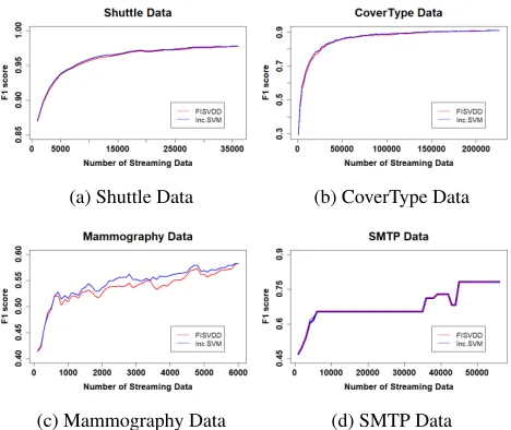
(a) Shuttle Data (b) CoverType Data
(c) Mammography Data (d) SMTP Data
Figure 1: F-1 Measure for Different Data Sets
in Section 4, FISVDD is faster because it is based solely on matrix manipulation and thus many calculations are saved.
Figure 1 shows plots of the F-1 measure (Tan, Steinbach, and Kumar 2007) of the accuracy of FISVDD and incremen-tal SVM with different training sizes. The plots show that by discarding interior points at the end of each iteration, there is almost no loss in the quality of outlier detection.
7
Conclusion
This paper introduces a fast incremental SVDD learning algorithm (FISVDD), which is more efficient than exist-ing SVDD algorithms. In each iteration, FISVDD considers only the incoming data point and the support vectors that were determined in the previous iteration. The essential cal-culations of FISVDD are contributed from incremental and decremental updates of a similar matrix inverseA−1. This algorithm builds on an observation that is natural in SVDD models but has not been fully utilized by existing SVDD al-gorithms: that all support vectors on the boundary have the same distance to the center of sphere in a higher-dimensional feature space as mapped by the Gaussian kernel function. FISVDD uses the signs of entries in the row sums ofA−1to
determine the interior points and support vectors and uses their magnitudes to determine the Lagrange multiplier αi
for each support vector. Experimental results indicate that FISVDD gains much efficiency with almost no loss in accu-racy and objective function value.
Acknowledgement
References
Ben-Hur, A.; Horn, D.; Siegelmann, H. T.; and Vapnik, V. 2001. Support vector clustering.Journal of Machine
Learn-ing Research2(Dec):125–137.
Cauwenberghs, G., and Poggio, T. 2001. Incremental and decremental support vector machine learning. InAdvances
in Neural Information Processing Systems, 409–415.
Evangelista, P.; Embrechts, M.; and Szymanski, B. 2007. Some properties of the Gaussian kernel for one class
learn-ing.Artificial Neural Networks–ICANN 2007269–278.
Gallier, J. 2010. The Schur complement and symmetric pos-itive semidefinite (and definite) matrices.Penn Engineering. Gu, B.; Sheng, V. S.; Tay, K. Y.; Romano, W.; and Li, S. 2015. Incremental support vector learning for ordinal regres-sion. IEEE Transactions on Neural Networks and Learning
Systems26(7):1403–1416.
Kakde, D.; Chaudhuri, A.; Kong, S.; Jahja, M.; Jiang, H.; and Silva, J. 2017. Peak criterion for choosing Gaussian ker-nel bandwidth in support vector data description. In Prog-nostics and Health Management (ICPHM), 2017 IEEE
In-ternational Conference on, 33–41. IEEE.
Laskov, P.; Gehl, C.; Kr¨uger, S.; and M¨uller, K.-R. 2006. Incremental support vector learning: Analysis, implemen-tation and applications. Journal of Machine Learning
Re-search7(Sep):1909–1936.
Lichman, M. 2013. UCI machine learning repository. Meyer, C. D. 2000. Matrix analysis and applied linear
al-gebra, volume 2. Siam.
Rayana, S. 2016. ODDS library.
Scheinberg, K. 2006. An efficient implementation of an active set method for SVMs. Journal of Machine Learning
Research7(Oct):2237–2257.
Sch¨olkopf, B.; Williamson, R. C.; Smola, A. J.; Shawe-Taylor, J.; and Platt, J. C. 2000. Support vector method for novelty detection. In Advances in Neural Information
Processing Systems, 582–588.
Smola, A. J., and Sch¨olkopf, B. 1998.Learning with kernels. GMD-Forschungszentrum Informationstechnik.
Syed, N. A.; Huan, S.; Kah, L.; and Sung, K. 1999. Incre-mental learning with support vector machines.
Tan, P.-N.; Steinbach, M.; and Kumar, V. 2007.Introduction
to data mining. Pearson Education India.
Tax, D. M. J., and Duin, R. P. W. 2004. Support vector data description. Machine learning54(1):45–66.
Tax, D. M. J., and Laskov, P. 2003. Online SVM learning: from classification to data description and back. InNeural Networks for Signal Processing, 2003. NNSP’03. 2003 IEEE
13th Workshop on, 499–508. IEEE.
Woods, K. S.; Doss, C. C.; Bowyer, K. W.; Solka, J. L.; Priebe, C. E.; and Kegelmeyer Jr, W. P. 1993. Compara-tive evaluation of pattern recognition techniques for detec-tion of microcalcificadetec-tions in mammography. International Journal of Pattern Recognition and Artificial Intelligence
7(06):1417–1436.
Xiao, Y.; Wang, H.; Zhang, L.; and Xu, W. 2014. Two meth-ods of selecting Gaussian kernel parameters for one-class SVM and their application to fault detection.