The Thirty-Third AAAI Conference on Artificial Intelligence (AAAI-19)
Learning to Solve NP-Complete
Problems: A Graph Neural Network for Decision TSP
Marcelo Prates,
∗1Pedro H. C. Avelar,
∗1Henrique Lemos,
∗1Luis C. Lamb,
1Moshe Y. Vardi
21Institute of Informatics, UFRGS, Porto Alegre, Brazil 2Dept. of Computer Science, Rice University, Houston, TX
[email protected], [email protected], [email protected], [email protected], [email protected]
Abstract
Graph Neural Networks (GNN) are a promising technique for bridging differential programming and combinatorial domains. GNNs employ trainable modules which can be assembled in different configurations that reflect the relational structure of each problem instance. In this paper, we show that GNNs can learn to solve, with very little supervision, the decision variant of the Traveling Salesperson Problem (TSP), a highly relevant
N P-Complete problem. Our model is trained to function as an effective message-passing algorithm in which edges (em-bedded with their weights) communicate with vertices for a number of iterations after which the model is asked to decide whether a route with cost< Cexists. We show that such a network can be trained with sets of dual examples: given the optimal tour costC∗, we produce one decision instance with target costx%smaller and one with target costx%larger thanC∗. We were able to obtain80%accuracy training with
−2%,+2%deviations, and the same trained model can gener-alize for more relaxed deviations with increasing performance. We also show that the model is capable of generalizing for larger problem sizes. Finally, we provide a method for pre-dicting the optimal route cost within2%deviation from the ground truth. In summary, our work shows that Graph Neu-ral Networks are powerful enough to solveN P-Complete problems which combine symbolic and numeric data.
Introduction
Deep learning has accomplished much in the last decade, advancing the state-of-the art of areas such as image recogni-tion (Krizhevsky, Sutskever, and Hinton 2012; Simonyan and Zisserman 2014; Li et al. 2015), natural language process-ing (Cho et al. 2014b; 2014a; Bahdanau, Cho, and Bengio 2014) and reinforcement learning (Mnih et al. 2013; 2015; Silver et al. 2016; 2017), which has been successfully com-bined with deep neural networks to master classic Atari games and yield superhuman performance in the Chinese boardgame Go (Mnih et al. 2013; 2015; Silver et al. 2016; 2017). However, the application of deep learning to sym-bolic domains directly, as opposed to their use in rein-forcement learning agents, is still incipient (d’Avila Garcez, Lamb, and Gabbay 2009; d’Avila Garcez et al. 2015; Evans and Grefenstette 2018).
∗
Equal contribution
Copyright c2019, Association for the Advancement of Artificial Intelligence (www.aaai.org). All rights reserved.
A promising meta-architecture to engineer models that learn on symbolic domains is to instantiate neural modules and assemble them in various configurations, each manifest-ing a graph representation of a given instance of the problem at hand (Scarselli et al. 2009). In this context, the neural com-ponents can be trained to learn to compute messages to send between nodes, yielding a differentiable message-passing algorithm whose parameters can be improved via gradient descent. This technique has been successfully applied to a growing range of problem domains, although with different names. Gilmer et al., which apply it to quantum chemistry problems, adopt the term “neural message passing” (Gilmer et al. 2017), while Palm et al. refer to “recurrent relational networks” in an attempt to train neural networks to solve Sudoku puzzles (Palm, Paquet, and Winther 2017).
A recent review of related techniques chooses the term
graph networks(Battaglia et al. 2018), but we shall refer to
graph neural networksnamed by Scarselli et al. who were among the first to propose such a model (Scarselli et al. 2009). Graph Neural Networks (GNNs) have recently been success-fully applied to the problem of predicting the boolean satis-fiability of a CNF formula, a very relevantN P-Complete combinatorial problem (SAT) (Selsam et al. 2018). Selsam et al. show that GNNs can be trained to obtain satisfactory accuracy (approximately85%) on small instances, and fur-ther that their performance can be improved by running the model for more message-passing timesteps. In addition, they show that satisfying assignments can be extracted from the network, which is never trained explicitly to produce them. The promising results ofNeuroSAT(as the authors named it) is an invitation to assess whether other hard combinatorial problems lend themselves to a simple GNN solution.
in addition to symbolic relationships (edges or connections). The traveling salesperson problem in its decision variant (does graphGadmit a Hamiltonian path with cost< C?) is a promising candidate, as it requires edge weightswias
well as the “target cost”Cto be taken under consideration to compute a solution.
The remainder of the paper is structured as follows. Next, we introduce a Graph Neural Network that shall be used in our TSP modelling. We then show how the proposed model learns to solve the Decision TSP and describe the experiments which validate the proposed model. Finally, we analyse the results and point out further research directions.
A GNN Model for the Decision TSP
Graph neural networks assign a multidimensional embed-ding∈Rdto each vertex in the graph representation of the problem instance at hand and perform a given number of message-passing iterations – in which a neural module com-putes a message from each embedding and sends it along its adjacencies. Each vertex accumulates its incoming messages by adding them up (or aggregating them through any other op-eration) and feeding the resultingRdvector into a RecurrentNeural Network (RNN) assigned with updating the embed-ding of said vertex. The only trainable parameters of such a model are the message computing modules and the RNN, so that conceptually what we have is a message-passing algo-rithm in which messages and updates are computed by neural networks.
Given a TSP instanceX = (G, C)composed of a graph G= (V,E)and a target costC∈R, we could assign an em-bedding to each vertex and send messages alongside edges, but all information about edge weights would be lost this way. Instead, we additionally assign embeddings toedges, which can be fed with their corresponding weights (edge embeddings in GNNs have shown promise in many applica-tions (Battaglia et al. 2018)). In this context, we replace the vertex-to-vertex adjacency matrixA∈ {0,1}|V|×|V|, by an edge-to-vertex adjacency matrixEV∈ {0,1}|E|×|V|, which connects each edgeei = (s, t, w)to its source and target
vertices. Because the model also needs to know the value of the target cost, we decided to feedCto each edge embedding alongside with its corresponding weight: given a target cost C, for each edgeei = (s, t, w)we concatenatewandCto
obtain a 2d vector∈R2. This vector is fed into a Multilayer perceptron (MLP) which expands it intoE(1)[i]∈
Rd, the initial embedding for edgeei. Following this initialization,
the model undergoes a given number of iterations in which vertices and edges exchange messages and refine their embed-dings, until finally the refined edge embeddings are fed into an MLP which computes a logit probability corresponding to the model’s prediction of the answer to the decision problem. In summary, upon training our proposed model learns seven tasks:
1. To produce a single Rd vector, which will be used to initialize all vertex embeddings
2. A functionEinit :R2→Rdto compute an initial edge embedding given the edge weightwand the route costC (MLP)
3. A functionVmsg : Rd → Rd to compute a message to send to edges given a vertex embedding (MLP)
4. A functionEmsg : Rd → Rdto compute a message to send to vertices given an edge embedding (MLP)
5. A functionVu:R2d→R2dto compute an updated vertex embedding (plus an updated RNN hidden state) given the current RNN hidden state and a message
6. A functionEu:R2d→R2dto compute an updated edge embedding (plus an updated RNN hidden state) given the current RNN hidden state and a message
7. A functionEvote:Rd→R1to compute a logit probabil-ity given an edge embedding (MLP)
Algorithm 1 briefly summarizes the proposed GNN-based procedure to solve the decision TSP. In the sequel, we shall illustrate how the model is used in learning route costs and validate our architecture.
Algorithm 1Graph Neural Network TSP Solver
1: procedureGNN-TSP(G= (V,E), C) 2:
3: // Compute binary adjacency matrix from edges to source & target vertices
4: EV[i, j]←1iff(∃v0|e
i=(vj, v0, w))| ∀ei∈E, vj∈V
5:
6: // Compute initial edge embeddings 7: E(1)[i]←E
init(w, C)| ∀ei= (s, t, w)∈ E
8:
9: // Runtmaxmessage-passing iterations
10: fort= 1. . . tmaxdo
11: // Refine each vertex embedding with messages received from edges in which it appears either as a source target vertex
12: Vh(t+1),V(t+1)←V
u(V
(t)
h ,EV T×E
msg(E
(t)))
13: // Refine each edge embedding with messages received from its source and its target vertex
14: E(ht+1),E(t+1)←E
u(E
(t)
h ,EV×msgV (V
(t)))
15: // Translate edge embeddings into logit probabilities 16: Elogits←Evote E(tmax)
17: // Average logits and translate to probability (the operatorhiindicates arithmetic mean)
18: prediction←sigmoid(hElogitsi)
Training the Model
performing the disjoint union between all graphs in the batch, yielding a “batch” graph withndisjoint subgraphs. Because subgraphs are disjoint, messages will not traverse through any pair of them, and there will be no change to the embedding refinement process as compared to a single run. There will be logit probabilities computed for each edge in the batch graph, which can be averaged among individual instances to compute a prediction for each one of them. The binary cross entropy can then be computed between these predictions and the corresponding decision problem solutions.
We produce training instances by samplingn∼ U(20,40) random points on a
√ 2 2 ×
√ 2
2 square and filling a distance matrixD ∈ Rn×n with the euclidean distance computed between each pair of points. These distances, by construction, are∈[0,1]. We also produce a complete adjacency matrix A∈ {0,1}n×n, and solve the corresponding TSP problem
using the Concorde TSP solver (Hahsler and Hornik 2007) to obtain optimal tour costs. A total of220such graphs were produced, from which we sample a total of1024per epoch to ensure that the probability of the model seeing the same graph twice at training time is kept low. Finally, for each graphG with optimal tour costC∗we produce two decision instances X+ = (G,1.02C∗)andX− = (G,0.98C∗)for which the answers are by construction YES and NO respectively. In doing so we effectively train the model to predict the decision problem within a2%positive or negative deviation from the optimal tour cost.
The model is instantiated with64-dimensional embeddings for vertices and edges and three-layered (64,64,64) MLPs with ReLU nonlinearities as the activations for all layers except for the last one, which has a linear activation. The model is run forTmax= 32time steps of message-passing.
Experimental Results and Analyses
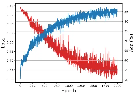
Upon2000training epochs, the model achieved80.16% ac-curacy averaged over the221 instances of the training set, having also obtained80%accuracy on a testing set of2048 instances it had never seen before. Instances from training and test datasets were produced with the same configura-tion (n∼ U(20,40)and2%percentage deviation). Figure 1 shows the evolution of the binary cross entropy loss and ac-curacy throughout the training process. Note that it is much easier to train the model with more relaxed deviations from the optimal cost, as Figure 2 shows.Extracting Route Costs
Now that we have obtained a solver for the decision TSP, we can exploit it to yield route cost predictions within a reasonable margin from the optimal cost. Figure 3 shows how the model behaves when it is asked to solve the decision problem for varying target costs. From its characteristic S-shape we can learn that the model feels confident that routes with too small costs do not exist and also confident that routes with too large costs do exist. Between these two regimes, the prediction undergoes a phase transition, with the model becoming increasingly unsure as we approach zero deviation from the optimal cost. In fact, this “acceptance curve” plotted for varying instance sizes is reminiscent of phase transitions
0 250 500 750 1000 1250 1500 1750 2000 Epoch
0.30 0.35 0.40 0.45 0.50 0.55 0.60 0.65 0.70
Lo
ss
50 55 60 65 70 75 80 85
A
cc
(
%
)
Figure 1: Evolution of the binary cross entropy loss (down-ward curve in red) and accuracy (up(down-ward curve in blue) throughout a total of2000training epochs on a dataset of220 graphs withn∼ U(20,40). Each graph with optimal TSP route costC∗is used to produce two instances to the TSP decision problem – “is there a route with cost<1.02C∗?” and “is there a route with cost < 0.98C∗?”, which are to be answered with YES and NO respectively. Each epoch is composed of128batches of16instances each (please note that at each epoch the network sees only a small sample of the dataset, and the accuracy here is computed relative to it).
on hard combinatorial problems such as SAT (Dudek, Meel, and Vardi 2016) and, along with a large number ofN P -Hard problems, the TSP itself has been shown to exhibit phase transition phenomena (Kirkpatrick and Toulouse 1985; Zhang 2004).
More importantly, we know from theoretical results that the average TSP tour length for a set ofnrandom (uniform) points on a plane is asymptotically proportional to√nwith the two-dimensional “TSP constant”β(2)as a proportional-ity factor (Beardwood, Halton, and Hammersley 1959). As a corollary, large instances allow for proportionally shorter routes than small instances1, a fact that, we believe, is man-ifest in the curves of Figure 3: for deviations close to zero, the model feels more confident that a route exists the larger the instance size is. As a result, the critical point (the devi-ation at which the model starts guessing YES) undergoes a left shift as the instance size increases, as seen in the curves’ derivatives in Figure 3.
In addition, all acceptance curves are above the50%line for deviation= 0, from which we conjecture that the trained model guesses by default that a routedoesexist and proceeds todisprovethis claim throughout message-passing iterations. Interestingly, this behavior is opposite to that of the GNN SAT-solverNeuroSAT (Selsam et al. 2018), which guesses UNSAT by default and changes its prediction only upon finding a satisfiable assignment. The factors determining
1 lim
n→∞C ∗
n/n= lim n→∞β(2)
√
n/n= 0whereCn∗is the optimal
0 200 400 600 800 1000 Epoch
50 60 70 80 90 100
A
cc
ur
ac
y
(%
)
dev=2.0% dev=5.0% dev=10.0%
Figure 2: The larger the deviation from the optimal cost, the faster the model learns: we were able to obtain>95% accuracy for10%deviation in 200 epochs. For5%, that per-formance requires double the time. For2%deviation, two thousand epochs are required to achieve85%accuracy.
which strategy the model will learn remain an open question, but we are hopeful that it is possible to engineer a training set to enforce that the model learns a negative-by-default algorithm.
To the best of our knowledge, the curves in Figure 3 become arbitrarily close to zero as we progress towards smaller deviations, but unfortunately the model starts to lose confidence that a route exists when it is fed with large target costs (≈ 100%deviation). This is probably due to the fact that, being trained with−2%,+2%deviations, the model has never seen target costs that large. Fortunately this can be corrected by re-training it for a single epoch with −2%,+2%,+100%,+200%,+1000%deviations, which is done with no significant effect to the test accuracy.
Intuitively, if we know nothing about the optimal cost, we can assume that we are closest to its value when the model’s
Algorithm 2Binary Search
1: procedureBINARY-SEARCH(G= (V,E),p,δ)
2: // Choose an initial guess for the optimal route cost. wn− andwn+ are the sets of the costs of thenedges
∈ Ewith smallest / largest costs respectively. 3: Cmin←Pwni−
4: Cmax←Pwin+
5: C∼ U(Cmin, Cmax)
6: whileCmin< C(1−δ)∨C(1 +δ)< Cmaxdo
7: ifGNN-TSP(G, C)< pthen 8: Cmin←C
9: else
10: Cmax←C
11: C←(Cmin+Cmax)/2
returnC
0 20 40 60 80 100
Pr
ed
ic
ti
on
(%
)
n=20 n=25 n=30 n=35 n=40
−0.10 −0.05 0.00 0.05 0.10
Deviation 0
500 1000
∂ ∂xPr
ed
ic
ti
on
(%
)
Figure 3: Average prediction obtained from the model as a function of the deviation between the target cost and the optimal cost for varying instance sizes (the pink band indi-cates the[−2%,+2%]interval). As expected, the curve is S-shaped, signalling that the model is very confident that routes with sufficiently large/small costs do/do not exist. The average prediction undergoes a phase transition as we tra-verse from negative to positive deviations. Larger instances exhibit smaller critical points, as evidenced by the left shifts on the derivatives of the acceptance curves in the bottom subfigure. The prediction for each deviation is averaged over 1024instances.
predictions are closest to50%. We can therefore guess an initial cost and perform a binary search on the x-axis of Figure 3. The procedure is detailed in Algorithm 2.
Instantiated withδ= 0.01and using the weights after the training and the single epoch of training for greater deviations, Algorithm 2 is able to predict route costs with on average 1.5%absolute deviation from the optimal, running for on average8.9iterations on the test dataset (1024n-city graphs withn∼ U(20,40)).
Model Performance on Larger Instances
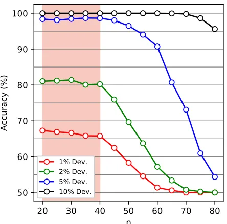
>80%accuracy throughout the range of sizes it was trained on, but loses performance progressively for larger problem sizes until it reaches the baseline of50%. Also, as expected given the acceptance curves in Figure 3, the model performs better for larger deviations (5%,10%) and worse for smaller ones (1%). Do note as well that a problem of double the size would require2nmore time to compute by traditional
algorithms, and thus such a rapid decay in accuracy is to be expected.
20 30 40 50 60 70 80
n 50
60 70 80 90 100
A
cc
ur
ac
y
(%
)
1% Dev. 2% Dev. 5% Dev. 10% Dev.
Figure 4: Accuracy of the trained model evaluated on datasets of1024instances with varying numbers of cities (n). The model is able to obtain > 80% accuracy for −2%,+2% deviation on the range of sizes it was trained on (painted in pink), but its performance degenerates progressively for larger instance sizes before reaching the baseline of50% atn≈75. Larger deviations yield higher accuracy curves, with the model obtaining>95%accuracy for−10%,+10% deviation even for the largest instance sizes.
Generalizing to Larger Deviations
Both the acceptance curves in Figure 3 and the accuracy curves in Figure 4 suggest that the model generalizes to larger deviations from the optimal tour cost than the2%it was trained on. In fact, these curves suggest that the model becomes more confident the larger the deviation is, which is not surprising given that the corresponding decision instances are comparatively more relaxed. Figure 5 shows how the accuracy increases until it plateaus at≈100%for increasing deviations and Table 1 depicts these results in the validation test sets.
Baseline Comparison
We chose to train the model on decision instances with −2%,+2%deviation from the optimal tour cost not because
Deviation Accuracy (%)
1 66
2 80
5 98
10 100
Table 1: Test accuracy averaged over1024n-city instances withn∼ U(20,40)for varying percentage deviations from the optimal route cost.
1 2 3 4 5 6 7 8 9 10
Deviation (%) 65
70 75 80 85 90 95 100
A
cc
ur
ac
y
(%
)
Figure 5: Accuracy of the trained model evaluated on the same test dataset of1024n-city instances withn∼ U(20,40) for varying deviations from the optimal tour cost. Although it was trained with target costs−2%,+2%from the optimal (dashed line), the model can generalize for larger deviations with increasing accuracy. Additionally, it could still obtain accuracies above the baseline (50%) for instances more con-strained than those it was trained on, with65%accuracy at −1%,+1%.
this was our intended performance, but because2%was the smallest deviation for which the network could be trained within reasonable time (≤2000epochs). For this reason, we do not know initially how the trained model compares with other methods. Although our goal is not to produce a state-of-the-art TSP solver but rather to demonstrate that neural networks can learn to solve this problem with very little super-vision (two bits: one bit for a positive solution and one bit for a negative one), we want to evaluate whether our model can outperform simple heuristics. We compare our model with (1) a Nearest Neighbor (NN) route construction and (2) a Simu-lated Annealing (SA) routine (Kirkpatrick, Gelatt, and Vecchi 1983). NN is arguably the simplest TSP heuristic, generally yielding low quality solutions. SA can generally produce good routes for the euclidean TSP, if the meta-parameters are calibrated correctly. We calibrate the SA’s initial tem-peratureT, cooling rateαand stopping temperatureTmin
with theiraceautomatic algorithm configuration package (L´opez-Ib´a˜nez et al. 2016).
heuris-tics could produce routes within a given deviation from the optimal route cost. This frequency can be thought as the TPR obtained by converting these methods into a predictor for the decision variant of the same problem (guess YES whenever you can constructively prove that a route within the target cost exists and NO otherwise). For the test dataset (1024n-city graphs withn∼ U(20,40)), Nearest Neighbor obtains on average routes20.2%more expensive than the op-timal, while Simulated Annealing brings that number down to6.7%. Nevertheless, for all tested deviations, the trained GNN model outperforms both methods, obtaining>90% TPR from deviations4%and above.
1 2 3 4 5 6 7 8 9 10
Deviation (%) 0
20 40 60 80 100
Tr
ue
Po
si
ti
ve
R
at
e
(%
)
GNN SA NN
Figure 6: Nearest Neighbor (NN) and Simulated Annealing (SA) do not yield a prediction for the decision variant of the TSP but rather a feasible route. To compare their performance with our model’s, we evaluate the frequency in which they yield solutions below a given deviation from the optimal route cost and plot alongside with the True Positive Rate (TPR) of our model for the same test instances (1024n-city graphs withn∼ U(20,40)).
Generalizing to Other Distributions
Although the model was trained on two-dimensional eu-clidean graphs, it can generalize, to some extent, to more comprehensive distributions. To evaluate this, we considered two families of graphs obtained from uniformly random dis-tance matrices: in the first distribution (“Rand.” in Table 2), edge weights are simply sampled uniformly at random; in the second (“Rand. Metric” in Table 2), edge weights are first sampled uniformly at random and then the metric property is enforced by replacing edge weights by the shortest path distance between the corresponding vertices. For2% devia-tion from the optimal tour cost, the model was able to obtain 64%accuracy on the random metric instances (versus80% on euclidean), but the performance is better for more relaxed deviations, with82%at5%and96%at10%deviation from the optimal route cost. The model was unable to achieve per-formance above the50%baseline for non-metric instances. We also evaluated the model with real world instances
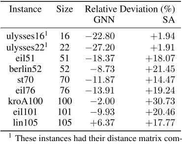
gath-ered from the Tsplib95 dataset (Reinelt 1995), for which the results obtained for the trained model with Algorithm 2 are reported in Table 3. In general, the model underestimates the optimal route cost, which is expected given the discussion in subsection onExtracting route costsabove. When the abso-lute relative deviation is considered, the GNN outperforms the SA routine for 6 out of 9 instances.
Deviation Accuracy (%)
Euc. 2D Rand. Metric Rand.
1 66 57 50
2 80 64 50
5 98 82 50
10 100 96 50
Table 2: Test accuracy averaged over1024n-city instances withn∼ U(20,40)for varying percentage deviations from the optimal route cost for differing random graph distribu-tions: two-dimensional euclidean distances, “random metric” distances and random distances.
Implementation and Reproducibility
The reproducibility of machine learning studies and experi-ments is relevant to the field of AI given the myriad of param-eters and implementation decisions one has to make. With this in mind, we summarize here the instantiation parameters of our model. The embedding size was chosen asd = 64, all message-passing MLPs are three-layered with layer sizes (64,64,64) with ReLU nonlinearities as the activation of all layers except the last one, which has a linear activation. The edge embedding initialization MLPs are three-layered with layer sizes (8,16,32) (we tried different architectures but have only obtained success with increasing layer sizes and a small initial layer). The kernel weights are initialized with TensorFlow’s Xavier initialization method described in (Glorot and Bengio 2010) and the biases are initialized with zeroes. The recurrent unit assigned with updating embed-dings is a layer-norm LSTM (Ba, Kiros, and Hinton 2016) with ReLU as its activation and both with kernel weights and biases initialized with TensorFlow’s Glorot Uniform Ini-tializer (Glorot and Bengio 2010), with the addition that the forget gate bias were increased by 1. The number of message-passing timesteps is set at tmax = 32. For each graph
in-stance, a pair of decision instances was created: a negative instance with target cost2%smaller than the optimal and a positive instance with target cost2%greater than the optimal. The training instances can be randomized but it is important that these pairs remain together in the same batch. Each train-ing epoch is composed by128Stochastic Gradient Descent operations on batches of16instance pairs (with a positive and with a negative deviation) each, randomly sampled from the training dataset.
Instance Size Relative Deviation (%)
GNN SA
ulysses161 16 −22.80 +1.94
ulysses221 22 −27.20 +1.91 eil51 51 −18.37 +18.07 berlin52 52 −8.73 +21.45
st70 70 −11.87 +14.47
eil76 76 −13.91 +19.24 kroA100 100 −2.00 +30.73 eil101 101 −9.93 +20.46 lin105 105 +6.37 +17.77
1 These instances had their distance matrix
com-puted according to Haversine formula (great-circle distance).
Table 3: The relative deviations from the optimal route cost are compared for the prediction obtained from the trained model with Algorithm 2 (GNN) and the Simulated Annealing heuristic (SA). Note that deviations obtained from the trained model are negative in general, as expected given the discus-sion in the subsection about Extracting route costs above.
information flow does not “spill” from one to another. Finally, on all experiments we have normalized all edge weights to be∈[0,1], and the target cost is always normalized by the number of citiesn. We have dedicated significant effort into making the reproduction of the experiments reported here available as a plug-and-play functionality. The code used to generate instances, train and evaluate the model and produce the figures presented in this paper is available at https://github.com/machine-reasoning-ufrgs/TSP-GNN.
Conclusions and Future Work
In this paper, we have proposed a Graph Neural Network (GNN) architecture which assigns multidimensional embed-dings to vertices and edges in a graph. In our model, vertices and edges undergo a number of message-passing iterations in which their embeddings are enriched with local informa-tion. Finally, each embedding “votes” on whether the graph admits a Traveling Salesperson route no longer thanC, and the votes are combined to yield a prediction. We show that such a network can be trained with sets of dual decision in-stances: given a optimal costC∗, we produce a (negative) instance with target costx%smaller and a (positive) instance with target costx%larger thanC∗. Upon training the model with−2%,+2%deviations were able to obtain80% accu-racy, and the model learned to generalize to larger deviations with increasing accuracy (96%at−5%,+5%). We also show how the model generalizes to some extent to larger problem sizes and different distributions. We conjecture that the model learns a positive-by-default algorithm, initially guessing that a route does exist and overriding that prediction when it can convince itself that is does not. In addition, the network is more confident that a route exists the larger the problem size is, which we think reflects the fact that the optimal TSP tour for a n-city euclidean graph scales with√n(and there-fore larger graphs admit proportionally shorter routes). By
plotting the “acceptance curves” of the trained model, we un-covered a behavior reminiscent of phase transitions on hard combinatorial problems. Coupled with a binary search, these curves allow for an accurate prediction of the optimal TSP cost, even though the network was only trained to provide yes-or-no answers.
We are hopeful that a training set can be engineered in such a way as to enforce the model to learn a negative-by-default algorithm, possibly enabling us to extract a TSP route from the refined embeddings as we know to be possible given the NeuroSAT experiment (Selsam et al. 2018). We intend on training and evaluating our model on a comprehensive set of real and random graphs, and to assess how far the model can generalize to larger problem sizes compared to those it was trained on. Finally, we believe that this experiment can showcase the potential of GNNs to the AI community and help promote an increased interest on integrated machine learning and reasoning models.
Acknowledgments
This research was partly supported by Coordenac¸˜ao de Aperfeic¸oamento de Pessoal de N´ıvel Superior (CAPES) - Finance Code 001 and by the Brazilian Research Council
CNPq.
References
Ba, J. L.; Kiros, J. R.; and Hinton, G. E. 2016. Layer normalization.arXiv preprint arXiv:1607.06450.
Bahdanau, D.; Cho, K.; and Bengio, Y. 2014. Neural machine translation by jointly learning to align and translate. arXiv preprint arXiv:1409.0473.
Battaglia, P. W.; Hamrick, J. B.; Bapst, V.; Sanchez-Gonzalez, A.; Zambaldi, V.; Malinowski, M.; Tacchetti, A.; Raposo, D.; Santoro, A.; Faulkner, R.; et al. 2018. Relational inductive biases, deep learning, and graph networks. arXiv preprint arXiv:1806.01261.
Beardwood, J.; Halton, J. H.; and Hammersley, J. M. 1959. The shortest path through many points. InMathematical Pro-ceedings of the Cambridge Philosophical Society, volume 55, 299–327. Cambridge University Press.
Cho, K.; van Merrienboer, B.; Bahdanau, D.; and Bengio, Y. 2014a. On the properties of neural machine trans-lation: Encoder-decoder approaches. In Proceedings of SSST@EMNLP 2014, Eighth Workshop on Syntax, Seman-tics and Structure in Statistical Translation, Doha, Qatar, 25 October 2014, 103–111.
d’Avila Garcez, A.; Lamb, L.; and Gabbay, D. 2009. Neural-Symbolic Cognitive Reasoning. Cognitive Technologies. Springer.
Dudek, J. M.; Meel, K. S.; and Vardi, M. Y. 2016. Combining the k-CNF and XOR phase-transitions. InProceedings of the Twenty-Fifth International Joint Conference on Artificial Intelligence, IJCAI 2016, New York, NY, USA, 9-15 July 2016, 727–734.
Evans, R., and Grefenstette, E. 2018. Learning explanatory rules from noisy data. JAIR61:1–64.
Gilmer, J.; Schoenholz, S. S.; Riley, P. F.; Vinyals, O.; and Dahl, G. E. 2017. Neural message passing for quantum chem-istry. InProceedings of the 34th International Conference on Machine Learning, ICML 2017, Sydney, NSW, Australia, 6-11 August 2017, 1263–1272.
Glorot, X., and Bengio, Y. 2010. Understanding the difficulty of training deep feedforward neural networks. In Proceed-ings of the Thirteenth International Conference on Artificial Intelligence and Statistics - AISTATS, 249–256.
Hahsler, M., and Hornik, K. 2007. Tsp-infrastructure for the traveling salesperson problem.Journal of Statistical Software
23(2):1–21.
Kingma, D. P., and Ba, J. 2014. Adam: A method for stochas-tic optimization.arXiv preprint arXiv:1412.6980.
Kirkpatrick, S., and Toulouse, G. 1985. Configuration space analysis of travelling salesman problems. Journal de Physique46(8):1277–1292.
Kirkpatrick, S.; Gelatt, C. D.; and Vecchi, M. P. 1983. Op-timization by simulated annealing.Science220(4598):671– 680.
Krizhevsky, A.; Sutskever, I.; and Hinton, G. E. 2012. Ima-genet classification with deep convolutional neural networks. InAdvances in neural information processing systems, 1097– 1105.
Li, H.; Lin, Z.; Shen, X.; Brandt, J.; and Hua, G. 2015. A convolutional neural network cascade for face detection. In
Proceedings of the IEEE Conference on Computer Vision and Pattern Recognition, 5325–5334.
L´opez-Ib´a˜nez, M.; Dubois-Lacoste, J.; P´erez C´aceres, L.; St¨utzle, T.; and Birattari, M. 2016. The irace package: Iter-ated racing for automatic algorithm configuration. Opera-tions Research Perspectives3:43–58.
Mnih, V.; Kavukcuoglu, K.; Silver, D.; Graves, A.; Antonoglou, I.; Wierstra, D.; and Riedmiller, M. 2013. Play-ing atari with deep reinforcement learnPlay-ing. arXiv preprint arXiv:1312.5602.
Mnih, V.; Kavukcuoglu, K.; Silver, D.; Rusu, A.; Veness, J.; Bellemare, M.; Graves, A.; Riedmiller, M.; Fidjeland, A.; Ostrovski, G.; et al. 2015. Human-level control through deep reinforcement learning. Nature518(7540):529.
Palm, R. B.; Paquet, U.; and Winther, O. 2017. Recurrent relational networks for complex relational reasoning.arXiv preprint arXiv:1711.08028.
Reinelt, G. 1995. Tsplib95. Interdisziplin¨ares Zentrum f¨ur Wissenschaftliches Rechnen (IWR), Heidelberg338.
Scarselli, F.; Gori, M.; Tsoi, A. C.; Hagenbuchner, M.; and Monfardini, G. 2009. The graph neural network model.IEEE Transactions on Neural Networks20(1):61–80.
Selsam, D.; Lamm, M.; Bunz, B.; Liang, P.; de Moura, L.; and Dill, D. L. 2018. Learning a SAT solver from single-bit supervision.arXiv preprint arXiv:1802.03685.
Silver, D.; Huang, A.; Maddison, C.; Guez, A.; Sifre, L.; Van Den Driessche, G.; Schrittwieser, J.; Antonoglou, I.; Panneershelvam, V.; Lanctot, M.; et al. 2016. Mastering the game of go with deep neural networks and tree search.
Nature529(7587):484.
Silver, D.; Schrittwieser, J.; Simonyan, K.; Antonoglou, I.; Huang, A.; Guez, A.; Hubert, T.; Baker, L.; Lai, M.; Bolton, A.; et al. 2017. Mastering the game of go without human knowledge. Nature550(7676):354.
Simonyan, K., and Zisserman, A. 2014. Very deep convo-lutional networks for large-scale image recognition. arXiv preprint arXiv:1409.1556.