The Thirty-Third AAAI Conference on Artificial Intelligence (AAAI-19)
How Many Pairwise Preferences Do We Need to Rank a Graph Consistently?
Aadirupa Saha
Department of CSAIndian Institute of Science, Bangalore aadirupa@iisc.ac.in
Rakesh Shivanna
Google Brain, Mountain Viewrakeshshivanna@google.com
Chiranjib Bhattacharyya
Department of CSA and Robert BoschCenter for Cyberphysical Systems Indian Institute of Science, Bangalore
chiru@iisc.ac.in
Abstract
We consider the problem of optimal recovery of true ranking ofnitems from a randomly chosen subset of their pairwise preferences. It is well known that without any further assump-tion, one requires a sample size ofΩ(n2)for the purpose. We
analyze the problem with an additional structure of relational graphG([n], E)over thenitems added with an assumption of locality: Neighboring items are similar in their rankings. Not-ing the preferential nature of the data, we choose to embed not the graph, but, itsstrong productto capture the pairwise node relationships. Furthermore, unlike existing literature that uses Laplacian embedding for graph based learning problems, we use a richer class of graph embeddings—orthonormal repre-sentations—that includes (normalized) Laplacian as its special case. Our proposed algorithm,Pref-Rank, predicts the under-lying ranking using an SVM based approach using the chosen embedding of the product graph, and is the first to provide statistical consistencyon two ranking losses:Kendall’s tau andSpearman’s footrule, with a requiredsample complexity ofO(n2χ( ¯G))23 pairs,χ( ¯G)being thechromatic numberof the complement graphG. Clearly, our sample complexity is¯ smaller for dense graphs, withχ( ¯G)characterizing the degree of node connectivity, which is also intuitive due to thelocality assumption e.g.O(n43)for union ofk-cliques, orO(n53)for random and power law graphs etc.—a quantity much smaller than the fundamental limit ofΩ(n2)for largen. This, for the first time, relates ranking complexity to structural properties of the graph. We also report experimental evaluations on dif-ferent synthetic and real-world datasets, where our algorithm is shown to outperform the state of the art methods.
1
Introduction
The problem of ranking from pairwise preferences has widespread applications in various real-world scenarios e.g. web search (Page et al. 1998; Kleinberg 1999), gene classi-fication, recommender systems (Theodoridis, Kotropoulos, and Panagakis 2013), image search (Geng, Yang, and Hua 2009) and more. Its of no surprise why the problem is so well studied in various disciplines of research, be that computer science, statistics, operational research or computational bi-ology. In particular, we study the problem of ranking (or
Copyright c2019, Association for the Advancement of Artificial Intelligence (www.aaai.org). All rights reserved.
A full version of this paper is available at http://arxiv.org/abs/ 1811.02161
ordering) of set ofnitems on a graph, given some partial information of the relative ordering of the item pairs.
It is well known from the standard results of classical sorting algorithms, for any set ofnitems associated to an un-known deterministic ordering, sayσ∗n, and given the learner has access to only preferences of the item pairs, in general one requires to observeΩ(nlogn)actively selected pairs (where the learner can choose which pair to observe next) to obtain the true underlying rankingσ∗
n; whereas, withrandom
selection of pairs, it could be as bad asΩ(n2).
Related Work.Over the years, numerous attempts have been made to improve the above sample complexities by imposing different structural assumptions on the set of items or the un-derlying ranking model. In active sampling setting, (Jamieson and Nowak 2011) gives a sample complexity ofO(dlog2n), provided the true ranking is realizable in a d-dimensional embedding; (Braverman and Mossel 2008) and (Ailon 2012) proposed a near optimal recovery with sample complexity ofO(nlogn)andO(npoly(logn))respectively, under noisy permutation and tournament ranking model. For the non-active (random) sampling setting, (Wauthier, Jordan, and Jojic 2013) and (Negahban, Oh, and Shah 2012) gave a sam-ple comsam-plexity bound ofO(nlogn)under noisy permutation (withO(logn)repeated sampling) and Bradley-Terry-Luce (BTL) ranking model. Recently, (Rajkumar and Agarwal 2016) showed a recovery guarantee ofO(nrlogn), given the preference matrix is rankrunder suitable transformation.
Table 1: Summary of sample complexities for ranking from pairwise preferences.
Reference Assumption on the Ranking Model Sampling Technique Sample Complexity
(Braverman and Mossel 2008) Noisy permutation Active O(nlogn)
(Jamieson and Nowak 2011) Lowd-dimensional embedding Active O(dlog2n)
(Ailon 2012) Deterministic tournament Active O(npoly(logn))
(Gleich and Lim 2011) Rank-rpairwise preference withνincoherence Random O(nνrlog2n)
(Negahban, Oh, and Shah 2012) Bradley Terry Luce (BTL) Random O(nlogn)
(Wauthier, Jordan, and Jojic 2013) Noisy permutation Random O(nlogn)
(Rajkumar and Agarwal 2016) Lowr-rank pairwise preference Random O(nrlogn)
(Niranjan and Rajkumar 2017) Lowd-rank feature with BTL Random O(d2logn)
(Agarwal 2010) Graph + Laplacian based ranking Random 7 Pref-Rank(This paper) Graph + Edge similarity based ranking Random O(n2χ( ¯G))2
3
generalization error bounds for the inductive and transductive graph ranking problems. (Agarwal and Chakrabarti 2007) de-rived generalization guarantees for PageRank algorithm. To the best of our knowledge, we are not aware of any literature which providestatistical consistencyguarantees to recover the true ranking and analyze the required sample complexity, which remains the primary focus of this work.
Problem Setting.We precisely address the question: Given the additional knowledge of a relational graph on the set ofn
items, sayG([n], E), can we find the underlying rankingσ∗n
efficiently (i.e. with a sample complexity less thanΩ(n2))? Of course, in order to hope for achieving a better sample complexity, there must be a connection between the graph and the underlying ranking – question is how to model this? A natural modelling could be to assume that similar items connected by an edge are close in terms of their rankings or similar node pairs have similar pairwise preferences e.g. In movie recommendations, if two moviesAandBbelongs to thriller genre andCbelongs to comedy, and it is known that
Ais preferred overC(i.e. the true ranking over latent topics prefers thriller over comedy), then it is likely thatBwould be preferred overC; and the learner might not require an explicit(B, C)labelled pair – thus one could hope to reduce the sample complexity by inferring preference information of the neighbouring similar nodes. However, how to impose such a smoothness constraint remains an open problem.
One way out could be to assume the true ranking to be a smooth function over the graph Laplacian as also assumed in (Agarwal 2010). However, why should we confine ourself to the notion of Laplacian embedding based similarity when several other graph embeddings could be explored for the purpose? In particular, we use a broader class oforthonormal representationof graphs for the purpose, which subsumes (normalized) Laplacian embedding as a special case, and assume the ranking to be asmooth functionwith respect to the underlying embedding (see Sec. 2.1 for details). Our Contributions.Under the smoothness assumptions, we show a sample complexity guarantee of O(n2χ( ¯G))23 to achieve ranking consistency – the result is intuitive as it indicates smaller sample complexity for densely connected graph, as one can expect to gather more information about the neighboring nodes compared to a sparse graph. Our pro-posedPref-Rankalgorithm, to the best of our knowledge, is the first attempt in provingconsistencyon a large class of graph families withϑ(G) =o(n), in terms ofKendall’s
tauandSpearman’s footrulelosses – It is developed on the novel idea of embedding nodes of the strong product graph
GG, drawing inference from the preferential nature of the data and finally uses a kernelized-SVM approach to learn the underlying ranking. We summarize our contributions:
• The choice of graph embedding: Unlike the existing lit-erature, which is restricted to Laplacian graph embed-ding (Ando and Zhang 2007), we choose to embed the strong productGGinstead ofG, as our ranking perfor-mance measures penalizes every pairwise misprediction; and use a general class of orthonormal representations, which subsumes (normalized) Laplacian as a special case.
• Our proposed preference based ranking algorithm: Pref-Rankis a kernelized-SVM based method that inputs an embedding of pairwise graphGG. The generalization error of Pref-Rankinvolves computing the transductive
Rademacher complexityof the function class associated with the underlying embedding used (see Thm. 3, Sec. 3).
• For the above, we propose to embed the nodes ofGG
with3 different orthonormal representations:(a) Kron-Lab(GG) (b)PD-Lab(G) and(c) LS-labelling; and derive generalization error bounds for the same (Sec. 4).
• Consistency:We prove the existence of an optimal embed-ding in Kron-Lab(GG) for whichPref-Rankis statis-tically consistent (Thm. 10, Sec. 5) over a large class of graphs, including power law and random graphs. To the best of our knowledge, this is the first attempt at establish-ing algorithmic consistency for graph rankestablish-ing problems.
• Graph Ranking Sample Complexity:Furthermore, we show that observingO(n2χ( ¯G))2
3 pairwise preferences is suffi-cient forPref-Rankto be consistent (Thm. 12, Sec. 5.1), which implies that adensely connected graph requires much smaller training data compared to a sparse graph
for learning the optimal ranking – as also intuitive. Our re-sult is the first to connect the complexity of graph ranking problem to its structural properties. Our proposed bound is a significant improvement in sample complexity (for
randomselection of pairs) for dense graphs e.g.O(n43)for union ofk-cliques; andO(n53)for random and power law graphs – a quantity much smaller thanΩ(n2).
Our experimental results demonstrate the superiority of
Inductive Pairwise Ranking (Niranjan and Rajkumar 2017) on various synthetic and real-world datasets; validating our theoretical claims. Table 1 summarizes our contributions.
2
Preliminaries and Problem Statement
Notations.Let[n] :={1,2, . . . , n}, forn∈Z+. Letxide-note theithcomponent of a vectorx∈
Rn. Let1{ϕ}denote
an indicator function that takes the value1, if the predicate
ϕis true and0otherwise. Let1ndenote ann-dimensional
vector of all1’s. LetSn−1=
u∈Rnkuk2= 1 denote a(n−1)dimensional sphere. For any matrixM∈Rm×n,
we denote theithcolumn byMi,∀i ∈[n]andλ1(M) ≥
. . .≥λn(M)to denote its sorted eigenvalues,tr(M)to be
its trace. LetS+
n ∈Rn×ndenote a set ofn×nsquare
sym-metric positive semi-definite matrices. LetG(V, E)denote a simple undirected graph, with vertex setV = [n]and edge setE⊆V ×V. We denote its adjacency matrix byAG. Let
¯
Gdenote the complement graph ofG, with the adjacency matrixAG¯ =1>n1n−I−AG,Ibeing the identity matrix. Orthonormal Representation of Graphs. (Lov´asz 1979) An orthonormal representation of G(V, E), V = [n] is
U = [u1, . . . ,un]∈Rd×nsuch thatu>i uj = 0whenever
(i, j)∈/ Eandui∈Sd−1, ∀i∈[n]. LetLab(G)denote the
set of all possible orthonormal representations ofGgiven byLab(G) :={U|U is an Orthonormal Representation}. Consider the set of graph kernelsK(G) :={K∈S+
n |Kii=
1,∀i ∈ [n]; Kij = 0,∀(i, j) ∈/ E}. (Jethava et al. 2013)
showed the two sets to be equivalent i.e. for every U ∈ Lab(G), one can constructK∈ K(G)and vice-versa.
Definition 1. Lov´asz Number.(Lov´asz 1979) Orthonormal representationsLab(G)of a graphGis associated with an interesting quantity – Lov´asz number ofG, defined as
ϑ(G) := min
U∈Lab(G)
min
c∈Sd−1maxi∈V
1 (c>u
i)2
Lov´asz Sandwich Theorem: If I(G)and χ(G)denote the independence number and chromatic number of the graphG, thenI(G)≤ϑ(G)≤χ( ¯G)(Lov´asz 1979).
Strong Product of Graphs.Given a graphG(V, E), strong product ofGwith itself, denoted byGG, is defined over the vertex setV(GG) = V ×V, such that two nodes
(i, j),(i0, j0) ∈ V(GG)is adjacent inGGiffi =i0
and(j, j0)∈E, or(i, i0)∈Eandj =j0, or(i, i0)∈Eand
(j, j0)∈E. Also, it is well known from the classical work of
(Lov´asz 1979) thatϑ(GG) =ϑ2(G).
2.1
Problem Statement
We study the problem of graph ranking on a simple, undi-rected graphG(V, E), V = [n]. Suppose there exists a true underlying ranking σ∗n ∈ Σn of the nodesV, whereΣn
is the set of all permutations of[n], such that for any two distinct nodesi, j ∈ V,iis said to be preferred overj iff
σ∗
n(i)< σn∗(j). Clearly, without any structural assumption
on how σ∗n relates to the underlying graph G(V, E), the knowledge ofG(V, E)is not very helpful in predictingσ∗n: Ranking on Graphs: Locality Property.A rankingσn is
said to havelocality propertyif∃at least one ranking function
f ∈Rnsuch thatf(i)> f(j)iffσ(i)< σ(j)and
|f(i)−f(j)| ≤c,whenever(i, j)∈E, (1)
wherec >0is a small constant that quantifies the “locality smoothness” off. One way is to modelfas a smooth function over the Laplacian embeddingL(Agarwal 2010) such that
f>Lf =P
(i,j)∈EAG(i, j) fi−fj 2
is small. However, we generalize this notion to a broader class of embeddings:
Locality with Orthonormal Representations:Formally, we try to solve for f ∈ RKHS(K)1 i.e.f = Kα, for some α ∈ Rn, where thelocalityhere impliesf to be a smooth
function over the embeddingK ∈ K(G), or alternatively
f>K†f ≤B, whereK†is the pseudo inverse ofKandB >
0is a small constant (details given in Appendix of the full arXiv version). Note that ifGis a completely disconnected graph, thenK(G) ={In}is the only choice forKandfi’s
are independent of each other, and the problem is as hard as the classical sorting ofnindependent items. But as the density ofGincreases, or equivalentlyϑ(G)≤χ( ¯G)n, thenK(G)becomes more expressive and the problem enters into an interesting regime, as the node dependencies come to play, aiding to faster learning rate. Recall that, however, we only have access toG, our task is to find a suitable kernelK
that fitsf onGand estimateσ∗naccurately.
Problem Setup. Consider the set of all node pairsPn =
(i, j) ∈ V ×Vi < j . Clearly |Pn| = n2
. We will use N = n2
and denote the pairwise preference label of the kth pair (i
k, jk) as yk ∈ {±1}, such that yk :=
sign(σ∗n(ik)−σn∗(jk)), ∀k∈[N]. The learning algorithm
is given access to a set of randomly chosen node-pairs
Sm ⊆ Pn, such that|Sm| = m ∈ [N]. Without loss of
generality, by renumbering the pairs we will assume the first
mpairs to be labelledSm ={(ik, jk)}mk=1, with the corre-sponding pairwise preference labelsySm = {yk}
m k=1, and set of unlabelled pairsS¯m =Pn\Sm ={(ik, jk)}Nk=m+1. GivenG,SmandySm, the goal of the learner is to predict
a rankingσˆn∈Σnover the nodesV, that gives an accurate
estimate of the underlying true rankingσ∗n. We use the follow-ing rankfollow-ing losses to measure performance (Monjardet 1998): Kendall’s Tau loss: dk(σ∗,σˆ) = N1
PN
k=11 (σ∗(ik)− σ∗(jk))(ˆσ(ik)−σˆ(jk)) < 0and Spearman’s Footrule
loss:ds(σ∗,σˆ) = n1Pni=1 σ
∗(i)−σˆ(i)
.dkmeasures the
average number of mispredicted pairs, whereasdsmeasures
the average displacement of the ranking order. By Diaconi-Graham inequality (Kumar and Vassilvitskii 2010), we know for anyσ,σ0∈Σn,dk(σ,σ0)≤ds(σ,σ0)≤2dk(σ,σ0).
Now instead of predictingσˆn∈Σn, suppose the learner
is allowed to predict a pairwise score functionf : Pn 7→
R\ {0}. Note, f = [fk]kN=1 ∈ (R\ {0})N can also be realized as a vector, wherefk denotes the score for every kthpair(i
k, jk), k∈[N]. We measure the prediction
accu-racy aspairwise(0-1)loss:`0−1(y
k, fk) = 1(fkyk <0),
or using the convex surrogate loss functions –hinge loss:
`hinge(y
k, fk) = (1−fkyk)+orramp loss:` ramp(y
k, fk) =
min{1,(1−fkyk)+}, where(a)+= max(a,0).
1
In general, given a transductive learning framework, fol-lowing the notations from (Ando and Zhang 2007; El-Yaniv and Pechyony 2007), for any pairwise preference loss`, we denote the empirical (training)`-error off aser`
Sm(f) =
1
m Pm
k=1`(yk, fk), the generalization (test set) error as er`
¯
Sm(f) =
1
N−m PN
k=m+1`(yk, fk)and the average pair-wise misprediction error aser`
n(f) =
1
N PN
k=1`(yk, fk).
2.2
Learners’ Objective - Statistical Consistency
for Graph Ranking from Pairwise Preferences
Let G be a graph family with infinite sequence of nodes
V = {vn}∞n=1. LetVn denote the firstn nodes ofV and Gn∈ Gbe a graph instance defined over (Vn, E1∪. . .∪En),
whereEnis the edge information of nodevnwith previously
observed nodesVn−1, n ≥ 2. Letσ∗n ∈ Σn be the true
ranking of the nodesVn. Now, givenGn andf ∈ (0,1)a
fixed fraction, letΠfbe a uniform distribution on the random
draw ofm(f) =dN fepairs of nodes fromN possible pairs
Pn. LetSm(f) = {(ik, jk) ∈ Pn} m(f)
k=1 be an instance of the draw, with corresponding pairwise preferencesySm(f) =
{yk} m(f)
k=1 . Given(Gn, Sm(f),ySm(f)), a learning algorithm Athat returns a rankingσˆnon the node setVnis said to be
statisticallyd-rank consistentw.r.t.Gif
P rSm(f)∼Πf(d(σ
∗
n,σˆn)≥)→0 as n→ ∞,
for any >0anddbeing the Kendall’s tau(dk)or
Spear-man’s footrule(ds)ranking losses. In the next section we
proposePref-Rank, an SVM based graph ranking algorithm and prove it to be statisticallyd-rank consistent (Sec. 5) with ‘optimal embedding’ in Kron-Lab(GG) (Sec. 4.1).
3
Pref-Rank
- Preference Ranking Algorithm
Given a graphG(V, E)and training set of pairwise prefer-ences(Sm,ySm), we design an SVM based ranking
algo-rithm that treats each observed pair inSm as a binary
la-belled training instance and outputs a pairwise score function
f ∈RN, which is used to estimate the final rankσˆ n. Step 1. Select an embedding (U˜): Choose a pairwise node embedding U˜ = [u˜1,· · ·˜uN] ∈ Rd×N, where any
node pair(ik, jk)∈ Pnis represented byu˜k, ∀k∈[N]. We
discuss the suitable embedding schemes in Sec. 4.
Step 2. Predict pairwise scores (f∗∈RN):We solve the
binary classification problem given the embeddingsU˜ and pairwise node preferences{(u˜k,yk)}mk=1using an SVM:
min
w∈Rd 1 2kwk
2 2+C
m X
k=1
`hinge(yk,w>u˜k) (2)
whereC >0is a regularization hyperparameter. Note that the dual of the above formulation is given by:
max α∈Rm+,kαk∞≤C
m X
k=1
αk−
1 2
m X
k,k0=1
αkαk0ykyk0K˜k,k0
whereK˜ =U˜>U˜ denotes the embedding kernel of the pair-wise node instances. From standard results of SVM, we know
that optimal solution of (2) givesw∗ =Pmk=1yk˜ukαk =
˜
Uβ, whereβ ∈ RN is such thatβk = ykαk, ∀k ∈ [m]
and0otherwise. Sinceyk ∈ {±1},kαk∞ =kβk∞ ≤C.
Thus for any k ∈ [N], the score of the pair (ik, jk) is
given byfk∗ =w∗>˜uk = Pm
l=1ylαlu˜>l ˜uk or equivalently
f∗=U˜>w∗ =U˜>Uβ˜ =Kβ˜ , which suggests the follow-ing alternative formulation of SVM:
max
f∈RN 1 2f
>K˜†f +C m X
k=1
`hinge(yk, fk) (3)
Clearly, iff∗denotes the optimal solution of (3), then we havef∗∈ {f |f =Kβ˜ , β∈RN, kβk
∞≤C}.
Remark 1. The regularizationf>K˜†f, precisely enforces thelocalityassumption of Sec. 2.1(see full version on arXiv).
Step 3. Predictσˆn ∈Σnfrom pairwise scoresf∗:Given
the score vector f∗ ∈ RN as computed above, predict a
rankingσˆn ∈Σnover the nodesV ofGas follows:
1. Letc(i)denote the number of wins of nodei∈V given by
P
{k=(ik,jk)|ik=i}
1 fk∗>0
+ P
{k=(ik,jk)|jk=i}
1 fk∗<0
.
2. Predict the ranking of nodes by sortingw.r.t. c(i), i.e. choose anyσˆn ∈ argsort(c), where argsort(c) = σ ∈
Σn|σ(i)< σ(j), ifc(i)> c(j), ∀i, j∈V .
A brief outline ofPref-Rankis given below:
Algorithm 1Pref-Rank
Input:G(V, E)and subset of preferences(Sm,ySm).
Init:Pairwise graph embeddingU˜ ∈Rd×N, d∈N+.
Getw∗by solving the SVM objective (2). Compute preference scoresf∗=U˜>w∗. Count number of winsc(i)for each nodei∈V:
c(i) := P {k=(ik,jk)|ik=i}
1 fk∗>0
+ P
{k=(ik,jk)|jk=i}
1 fk∗<0
Return:Ranking of nodesσˆn ∈argsort(c).
3.1
Generalization Error of
Pref-Rank
We now derive generalization guarantees ofPref-Rankon its test set errorer`ρ
¯
Sm(f
∗) = 1
N−m PN
k=m+1`
ρ(y
k, fk∗),w.r.t.
some loss function`ρ : {±1} ×
R7→ R+, where`ρis
as-sumed to beρ-lipschitz (ρ >0) with respect to its second argument i.e.|`ρ(y
k, fk)−`ρ(yk, fk0)| ≤
1
ρ|fk−f 0 k|, where
f,f0 :Pn 7→RN be any two pairwise score functions. We
find it convenient to define the following function class com-plexity measure associated with orthonormal embeddings of pairwise preference strong product of graphs (as motivated in (Pelckmans, Suykens, and Moor 2007)):
Definition 2 (Transductive Rademacher Complexity).
Given a graphG(V, E), letU˜ ∈ Rd×N be any pairwise
h : col(U˜) 7→ R} associated with U˜, its transductive
Rademacher complexity is defined as
R(HU˜,U˜, p) =
1
NEγ "
sup
h∈HU˜
N X
k=1
γkh(˜uk) #
,
where for any fixedp ∈ (0,1/2],γ = (γ1, . . . , γN) is a
vector ofi.i.d.random variables such thatγi∼ {+1,−1,0}
with probabilityp,pand1−2prespectively.
We bound the generalization error ofPref-Rankin terms of the Rademacher complexity. Note the result below crucially depends on the fact that any score vectorf∗returned by Pref-Rank, is of the formf∗ = U˜>w∗, for somew∗ ∈ {h |
h=Uβ˜ ,β∈RN,kβk
∞≤C}, whereU˜ ∈Rd×N be the
embedding used inPref-Rank(refer (2), (3) for details). Theorem 3(Generalization Error ofPref-Rank). Given a graphG(V, E), letU˜ ∈Rd×N be any pairwise embedding
ofG. For anyf ∈ (0,1/2], let Πf be a uniform
distribu-tion on the random draw ofm(f) =dN fepairs of nodes fromPn, such thatSm(f) = {(ik, jk) ∈ Pn}
m(f)
k=1 ∼ Πf,
with corresponding pairwise preferenceySm(f). LetS¯m(f)=
Pn\Sm(f). LetHU˜ ={w|w=Uβ˜ , β ∈RN, kβk∞≤ C, C >0}and`ρ :{±1} ×
R7→[0, B]be a bounded,ρ
-Lipschitz loss function. Then for anyδ >0, with probability
≥1−δoverSm(f)∼Πf,
er`S¯ρm(f)(f
∗)≤er`ρ
Sm(f)(f
∗)+R(HU˜,U˜, p)
ρf(1−f) +
C1B
q
ln 1δ
(1−f)√N f,
wherep =f(1−f)andf∗ = U˜>w∗ ∈ RN is pairwise
score vector output by Pref-Rank andC1>0is a constant. Remark 2. It might appear from above that a higher value ofR(HU˜,U˜, p)leads to increased generalization error. How-ever, note that there is atradeoffbetween the first and second term, since a higher Rademacher complexity implies a richer function classHU˜, which in turn is capable of producing a better prediction estimatef∗ =U˜>w, resulting in a much lower training set errorer`ρ
Sm(f)(f
∗). Thus, ahigher value of
R(HU˜,U˜, p)is desiredfor better generalization.
Taking insights from Thm. 3, it follows that the perfor-mance ofPref-Rankcrucially depends on theRademacher complexityR(HU˜,U˜, p) of the underlying function class
HU˜, which boils down to the problem of finding a “good” embeddingU˜. We address this issue in the next section.
4
Choice of Embeddings
We discuss different classes of pairwise graph embeddings and their generalization guarantees. Recalling the results of (Ando and Zhang 2007) (see Thm.1), which provides a cru-cial characterization of the class of optimal embeddings for any graph based regularization algorithms, we choose to work with embeddings with normalized kernels, i.e.K˜ =U˜>U˜
such thatK˜kk= 1,∀k∈[N]. The following theorem
analy-ses the Rademacher complexity of ‘normalized’ embeddings:
Theorem 4 (Rademacher Complexity of Orthonormal Embeddings). GivenG(V, E), letU˜ ∈Rd×N be any
‘nor-malized’ node-pair embedding ofGG, letK˜ =U˜>U˜
be the corresponding graph-kernel, thenR(HU˜,U˜, p) ≤
C q
2pλ1(K˜), whereλ1(K˜)is the largest eigenvalue of K˜. Note that the above result does not educate us on the choice ofU˜ – we impose more structural constraints and narrow down the search space of optimal ‘normalized’ graph embed-dings and propose the following special classes:
4.1
Kron-Lab(
G
G
): Kronecker Product
Orthogonal Embedding
Given any graph G(V, E), with U = [u1,u2, . . . ,un] ∈
Rd×nbeing an orthogonal embedding ofG, i.e.U∈Lab(G),
its Kronecker Product Orthogonal Embedding is given by:
Kron-Lab(GG):={U˜ ∈Rd2×n2
|U˜ =U⊗U,
U∈Rd×nsuch thatU∈Lab(G)},
where⊗is the kronecker (or outer) product of two matrix. The‘niceness’of the above embedding lies in the fact that one can construct U˜ ∈ Kron-Lab(GG) from any or-thogonal embedding of the original graphU ∈Lab(G)– letK :=U>UandK˜ :=U˜>U˜, we see that for any two
k, k0 ∈[n2],K˜
kk0 =u˜>
k˜u 0
k = (uik⊗ujk)
>(u
ik0⊗ujk0) = (u>
ikuik0)(u
>
jkujk0) = Kikik0Kjkjk0, where (i(·), j(·)) ∈ [n]×[n]are the node pairs corresponding tok, k0. Hence,
˜
K = K⊗K. Note that whenk =k0, we haveK˜kk = 1,
asU ∈Lab(G)andKii = 1,∀i ∈ [n]. This ensures that
the kronecker product graph kernelK˜ satisfies the optimality criterion of ‘normalized’ embedding as previously discussed.
Lemma 5 (Rademacher Complexity of
Kron-Lab(G G)). Consider any U ∈ Lab(G),
K = U>U and the corresponding U˜ ∈ Kron-Lab(G G). Then for any p ∈ (0,1/2] and
HU˜ ={w|w=Uβ˜ , β∈R
N, kβk∞≤C, C >0}we
have,R(HU˜,U˜, p)≤Cλ1(K)
√
2p.
Above leads to the following generalization guarantee: Theorem 6 (Generalization Error of Pref-Rank with Kron-Lab(GG)). For the setting as in Thm. 3 and Lem. 5, for anyU˜ ∈Kron-Lab(GG), we have
er`S¯ρ(f∗)≤er`
ρ
S (f
∗) + Cλ1(K)
√
2
ρpf(1−f)+
C1B
1−f s
log(1δ)
N f
4.2
Pairwise Difference Orthogonal Embedding
Given graphG(V, E), let U = [u1,u2, . . . ,un] ∈ Rd×n
be such thatU∈Lab(G). We define the class ofPairwise Difference Orthogonal EmbeddingsofGas:
PD-Lab(G):={U˜ ∈Rd×N |u˜
ij=ui−uj∀(i, j)∈ Pn,
U∈Rd×nsuch thatU∈Lab(G)}
LetE= [ei−ej](i,j)∈Pn ∈ {0,±1}
n×N, wheree
idenotes
thatU˜ =UE∈PD-Lab(G) and the corresponding graph
kernel is given byK˜ =E>KE. For PD embedding, we get:
Lemma 7(Rademacher Complexity of PD-Lab(G)). Con-sider anyU ∈ Lab(G),K = U>U and the correspond-ing U˜ ∈ PD-Lab(G). Then for any p ∈ (0,1/2] and
HU˜ ={w|w=Uβ˜ , β∈RN, kβk2≤tC
√
N , C >0}, we haveR(HU˜,U˜, p)≤2C
p
pnλ1(K).
Similarly as before, using above result we can show that:
Theorem 8 (Generalization Error of Pref-Rank with PD-Lab(G)). For the setting as in Thm. 3 and Lem. 7, for anyU˜ ∈PD-Lab(G), we have
er`S¯ρ(f
∗)≤er`ρ
S(f∗) +
2Cpnλ1(K)
ρpf(1−f) +
C1B
1−f s
log(1δ)
N f
Recall from Thm. 3 thatf∗=U˜>w. Thus the‘niceness’
of PD-Lab(G) lies in the fact that it comes with the free transitivity property – for any two node pairsk1:= (i, j)and
k2 := (j, l), iff∗ scores nodeihigher thanji.e.fk∗1 >0, and nodejhigher than nodeli.e.fk∗
2 >0; then for any three nodesi, j, l∈[n], this automatically impliesfk∗
3 >0, where
k3:= (i, l)i.e. nodeigets a score higher than nodel.
Remark 3. Although Lem. 5 and 7 shows that both Kron-Lab(GG) and PD-Lab(G) are associated to rich expres-sive function classes with high Rademacher complexity,the superiority of Kron-Lab(GG) comes with an additional consistency guarantee, as we will derive in Sec. 5.
4.3
LS
-labelling based Embedding
The embedding (graph kernel) corresponding to LS -labelling (Luz and Schrijver 2005) of graphGis given by:
KLS(G) =
AG
τ +In, whereτ≥ |λn(AG)|, (4)
whereAGis the adjacency matrix of graphG. It is known
thatKLS ∈Rn×nis symmetric and positive semi-definite,
and hence defines a valid graph kernel; also∃ULS∈Lab(G)
such thatU>LSULS=KLS. We denoteULSto be the
cor-responding embedding matrix forLS-labelling. We define
LS-labelling of the strong product of graphs as:
˜
KLS(GG) =KLS(G)⊗KLS(G) (5)
and equivalently, the embedding matrix U˜LS(GG) =
ULS(G)⊗ULS(G). Similar to Kron-Lab(GG), we have
˜
KLS(k, k) = 1, ∀k ∈ [n2], sinceKLS(i, i) = 1, ∀i ∈
[n]. Following result shows that K˜LS(GG) has high
Rademacher complexity on randomG(n, q)graphs.
Lemma 9. Let G(n, q)be a Erd´os-R´eyni random graph, where each edge is present independently with probability
q∈[0,1], q=O(1). Then, the Rademacher complexity of the function class associated withK˜LS(GG)isO(
√ n).
Laplacian based Embedding. This is the most popular choice of graph embedding that uses the inverse of the Lapla-cian matrix for the purpose. Formally, let di denotes the
degree of vertexi∈[n]in graphG, i.e.di= (AG)>i 1n, and
Ddenote a diagonal matrix such thatDii = di,∀i ∈ [n].
Then, the Laplacian and normalized Laplacian kernel of
G is defined as follows2: K
Lap(G) = (D−AG)† and
KnLap(G) = (In −D−1/2AGD−1/2)†. Though widely
used (Agarwal 2010; Ando and Zhang 2007), it is not very expressive on dense graphs with highχ(G)– we observe that the Rademacher complexity of function class associated with Laplacian is an order magnitude smaller than that of
LS-labelling. See full version on arXiv for details.
5
Consistency with Kron-Lab(
G
G
)
In this section, we show thatPref-Rankis provably statisti-cally consistent while working withkronecker product or-thogonal embeddingKron-Lab(GG)(see Sec. 4.1). Theorem 10 (Rank-Consistency). For the setting as in Sec. 2.2, there exists an embeddingU˜n∈Kron-Lab(Gn Gn) such that, if σn ∈ RN denotes the pairwise scoresreturned by Pref-Rank on input(U˜n, Sm(f),ySm(f)), then
∀Gn ∈ G, with probability≥
1− 1
N
overSm(f)∼Πf
d(σ∗n,σˆn) =O
ϑ(G n) nf
s
1−f f
12
+
s
lnn N f
!
,
whereddenotes Kendall’s tau(dk)or Spearman’s footrule
(ds)ranking loss functions.
Consistency follows from the fact that for large families of graphs including random graphs (Coja-Oghlan 2005) and power law graphs (Jethava et al. 2013),ϑ(Gn) =o(n).
5.1
Sample Complexity for Ranking Consistency
We analyze the minimum fraction of pairwise node pref-erencesf∗ to be observed for Pref-Rankalgorithm to be statistically ranking consistent. We refer the required sample sizem(f∗) =dN f∗easranking sample complexity.
Lemma 11. IfGin Thm. 10 is such thatϑ(Gn) =nc,0≤
c <1, then observing onlyf∗=O
√
ϑ(Gn)
n12−ε
43
fraction of pairwise node preferences is sufficient for Pref-Rank to be statistically ranking consistent, for any0< ε < (1−2c).
Note that one could potentially choose anyε∈ 0,1−2c
for the purpose – thetradeoff lies in the fact that a higher
εleads tofaster convergence rate ofd(σ∗n,σˆn) = O(n1ε),
although at thecost of increased sample complexity; on the contrary setting ε → 0 gives a smaller sample complex-ity, with significantly slower convergence rate (see proof of Lem. 11 in the full version). We further extend Lem. 11 and relate ranking sample complexity to structural properties of the graph –coloring numberof the complement graphχ( ¯G).
Theorem 12. Consider a graph familyGsuch thatχ( ¯Gn) = o(n),∀Gn ∈ G. Then observingO(n2χ( ¯G))
2
3 pairwise
pref-erences is sufficient for Pref-Rank to be ranking consistent.
2†
Above conveys that fordense graphs we need fewer pair-wise samples compared to sparse graphsasχ( ¯G)reduces with increasing graph density. We discuss the sample com-plexities for some special graphs below whereϑ(G) =o(n).
Corollary 13(Ranking Consistency on Special Graphs).
Pref-Rank algorithm achieves consistency on the follow-ing graph families, with the required sample complexities –
(a)Complete graphs:O(n43) (b)Union ofkdisjoint cliques:
O(n43k 2
3) (c) Complement of power-law graphs: O(n 5 3)
(d)Complement ofk-colorable graphs:O(n43k 2
3) (e)Erd˝os R´eyni randomG(n, q)graphswithq=O(1):O(n53). Remark 4. Thm. 10 along with Lem. 11 suggest that if the graph satisfies a crucial structural property:ϑ(G) =o(n)and given sufficient sample ofΩ(n2ϑ(G))2
3 pairwise preferences,
Pref-Rankyields consistency. Note thatϑ(G)≤χ( ¯G)≤n, where the last inequality is tight for completely disconnected graph – which implies one need to observeΩ(n2)pairs for consistency, as a disconnected graph does not impose any structure on the rank. Smaller theϑ(G), denser the graph and we attain consistency observing a smaller number of node pairs, the best is of course is whenGis a clique, asϑ(G) = 1! Thus, for sparse graphs withϑ(G) = Θ(n), consistency and learnability is far fetched without observingΩ(n2)pairs.
Note that proof of Thm. 10 relies on the fact that the maximum SVM margin attained for the formulation (2) is
ϑ(GG), which is achieved byLS-labelling on Erd˝os R´eyni random graphs (Shivanna and Bhattacharyya 2014); and thus guarantee consistency, withO(n53)sample complexity.
6
Experiments
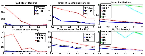
We conducted experiments on both real-world and synthetic graphs, comparingPref-Rankwith the following algorithms: Algorithms.(a)PR-Kron: Pref-Rank withK˜LS(GG)
(see Eqn. (5))(b)PR-PD:Pref-Rank with PD-Lab(G) with
LS-labelling i.e.U=ULS,(c)GR: Graph Rank (Agarwal
2010),(d)RC: Rank Centrality (Negahban, Oh, and Shah 2012) and(e)IPR: Inductive Pairwise Ranking, with Lapla-cian as feature embedding (Niranjan and Rajkumar 2017).
Recall from the list of algorithms in Table 1. Except (Agar-wal 2010), none of the others applies to ranking on graphs. Moreover, they work under specific models, e.g.noisy permu-tations(Wauthier, Jordan, and Jojic 2013), (Rajkumar and Agarwal 2016) requires knowledge of the preference matrix rank. Nevertheless, we compare with Rank Centrality (works under BTL model) and Inductive Pairwise Ranking (requires item features), but as expected both perform poorly. Performance Measure.Note the generalization guarantee of Thm. 3 not only holds for full ranking but for any gen-eral preference learning problem, where the nodes ofGare assigned to an underlying preference vectorσ∗n∈Rn.
Sim-ilar as before, the goal is to predict a pairwise score vector
f ∈RN to optimize the average pairwise mispredictionsw.r.t.
some loss function`:{±1} ×R\ {0} 7→R+defined as:
er`D(f) = 1
|D| X
k∈D
`(yk, fk), (6)
whereD={(ik, jk)∈ Pn|σn∗(ik)6=σ∗n(jk), k∈[N]} ⊆ Pn denotes the subset of node pairs with distinct
prefer-ences andyk = sign(σn∗(jk)−σn∗(ik)), ∀k ∈ D. In
par-ticular,Pref-Rank applies tobipartite ranking(BR), where
σ∗n∈ {±1}n,categorical ord-class ordinal ranking(OR),
whereσ∗n∈[d]n, d < n, and the originalfull ranking(FR) problem as motivated in Sec. 2.1. We consider all three tasks withpairwise0-1loss, i.e.`(yk, fk) =1(ykfk <0).
6.1
Synthetic Experiments
Graphs.We use3types of graphs, each withn= 30nodes:
(a)Union ofk-disconnected cliqueswithk= 2and10,(b)
r-Regular graphswithr= 5and15; and(c)G(n, q)Erd˝os R´eyni random graphswith edge probabilityq= 0.2and0.6.
Figure 1: Synthetic Data: Average number of mispredictions (erD`0-1(f), Eqn. (6)) vs fraction of sampled pairs(f).
Generatingσ∗n.For each of the above graphs, we compute
f∗ =AGα, whereα ∈[0,1]n is generated randomly, and
setσ∗n =argsort(f∗)(seePref-Rank, Step3for definition).
We report the average performance across 10repeated runs in Fig. 6.1. In all the cases, our proposed algorithms PR-KronandPR-PDoutperforms the rest, withGRperforming competitively. As expected,RCandIPRperform poorly as they could not exploit the underlying graphlocalityproperty.
6.2
Real-World Experiments
Datasets.We use6standard real-world datasets3for three graph learning tasks –(a)HeartandFourclassforBR,(b)
VehicleandVowelforOR, and(c)HouseandMgforFR. Graph Generation. For each dataset, we select 10 ran-dom subsets of 40 items each and construct a similarity matrix using RBF kernel, where (i, j)th entry is given by
exp −kxi−xjk2
2µ2
,xibeing the feature vector andµthe
av-erage distance. For each of the10subsets, we constructed a graph by thresholding the similarity matrices about the mean. Generatingσ∗n.For each dataset, the provided item labels are used as the score vectorf∗and we setσ∗n=argsort(f∗).
For each of the task, we report the average error across10
randomly drawn subsets in Fig. 6.2. As before, our proposed methodsPR-KronandPR-PDperform the best, followed byGR. Once againRCandIPRperform poorly4. Note that, the performance error increases from bipartite ranking(BR) to full ranking(FR), former being a relatively simpler task.
3
https://www.csie.ntu.edu.tw/∼cjlin/libsvmtools/datasets/
4
Results on more datasets are provided in the supplementary of the full version on arXiv.
Figure 2: Real-World Data: Average number of mispredic-tions (er`0-1
D (f), Eqn. (6)) vs fraction of sampled pairs(f).
7
Conclusion and Future Work
In this paper we address the problem of ranking nodes of a graphG([n], E)given a random subsample of their pair-wise preferences. Our proposedPref-Rankalgorithm, guar-antees consistency with a required sample complexity of
O n2χ( ¯G)23 – also gives novel insights by relating the ranking sample complexity with graph structural properties through the chromatic number ofG¯, i.e.χ( ¯G), for the first time. One possible future direction is to extend the setting to noisy preferences e.g. using BTL model (Negahban, Oh, and Shah 2012), or analyse the problem with other measures of ranking losses e.g. NDCG, MAP (Agarwal 2008). Fur-thermore, proving consistency ofPref-Rankalgorithm using PD-Lab(G) also remains an interesting direction to explore.
Acknowledgements
Thanks to the anonymous reviewers for their insightful com-ments. This work is partially supported by an Amazon grant to the Department of CSA, IISc and Qualcomm travel grant.
References
Agarwal, A., and Chakrabarti, S. 2007. Learning Random Walks to Rank Nodes in Graphs. InProceedings of the 24th international conference on Machine learning, 9–16. ACM.
Agarwal, S. 2008. Transductive Ranking on Graphs.Tech Report. Agarwal, S. 2010. Learning to Rank on Graphs.Machine learning 81(3):333–357.
Ailon, N. 2012. An Active Learning Algorithm for Ranking from Pairwise Preferences with an Almost Optimal Query Complexity. Journal of Machine Learning Research13(Jan):137–164.
Ando, R. K., and Zhang, T. 2007. Learning on Graph with Laplacian Regularization. InAdvances in Neural Information Processing Systems, 25–32.
Braverman, M., and Mossel, E. 2008. Noisy Sorting without Resampling. InProceedings of the nineteenth annual ACM-SIAM symposium on Discrete algorithms, 268–276. Society for Industrial and Applied Mathematics.
Coja-Oghlan, A. 2005. The Lov´asz Number of Random Graphs. Combinatorics, Probability and Computing14(04):439–465. Del Corso, G. M., and Romani, F. 2016. A Multi-class Approach for Ranking Graph Nodes: Models and Experiments with Incomplete Data.Information Sciences329:619–637.
El-Yaniv, R., and Pechyony, D. 2007. Transductive Rademacher Complexity and its Applications. InLearning Theory. Springer. Geng, B.; Yang, L.; and Hua, X.-S. 2009. Learning to Rank with Graph Consistency.
Gleich, D. F., and Lim, L.-h. 2011. Rank Aggregation via Nuclear Norm Minimization. InProceedings of the 17th ACM SIGKDD In-ternational Conference on Knowledge Discovery and Data Mining. He, X.; Gao, M.; Kan, M.-Y.; and Wang, D. 2017. BiRank: Towards Ranking on Bipartite Graphs. IEEE Transactions on Knowledge and Data Engineering29(1):57–71.
Hsu, C.-C.; Lai, Y.-A.; Chen, W.-H.; Feng, M.-H.; and Lin, S.-D. 2017. Unsupervised Ranking using Graph Structures and Node At-tributes. InProceedings of the Tenth ACM International Conference on Web Search and Data Mining, 771–779. ACM.
Jamieson, K. G., and Nowak, R. 2011. Active Ranking using Pair-wise Comparisons. InAdvances in Neural Information Processing Systems, 2240–2248.
Jethava, V.; Martinsson, A.; Bhattacharyya, C.; and Dubhashi, D. P. 2013. Lov´aszϑFunction, SVMs and Finding Dense Subgraphs. Journal of Machine Learning Research14(1):3495–3536. Kleinberg, J. M. 1999. Authoritative Sources in a Hyperlinked Environment.Journal of the ACM (JACM)46(5):604–632. Kumar, R., and Vassilvitskii, S. 2010. Generalized Distances between Rankings. InProceedings of the 19th international confer-ence on World wide web, 571–580. ACM.
Lov´asz, L. 1979. On the Shannon Capacity of a Graph.Information Theory, IEEE Transactions on25(1):1–7.
Luz, C. J., and Schrijver, A. 2005. A Convex Quadratic Charac-terization of the Lov´asz Theta Number.SIAM Journal on Discrete Mathematics19(2):382–387.
Monjardet, B. 1998. On the Comparison of the Spearman and Kendall Metrics between Linear Orders.Discrete mathematics. Negahban, S.; Oh, S.; and Shah, D. 2012. Iterative Ranking from Pair-wise Comparisons. InAdvances in Neural Information Pro-cessing Systems, 2474–2482.
Niranjan, U., and Rajkumar, A. 2017. Inductive Pairwise Ranking: Going Beyond thenlog(n)Barrier. InAAAI, 2436–2442. Page, L.; Brin, S.; Motwani, R.; and Winograd, T. 1998. The PageR-ank Citation RPageR-anking: Bringing Order to the Web. InProceedings of the 7th International World Wide Web Conference, 161–172. Pelckmans, K.; Suykens, J. A.; and Moor, B. 2007. Transductive Rademacher Complexities for Learning over a Graph. InMLG. Rajkumar, A., and Agarwal, S. 2016. When Can We Rank Well from Comparisons ofO(nlogn)Non-Actively Chosen Pairs? In Conference on Learning Theory, 1376–1401.
Shivanna, R., and Bhattacharyya, C. 2014. Learning on Graphs Using Orthonormal Representation is Statistically Consistent. In Advances in Neural Information Processing Systems, 3635–3643. Theodoridis, A.; Kotropoulos, C.; and Panagakis, Y. 2013. Mu-sic Recommendation Using Hypergraphs and Group Sparsity. In Acoustics, Speech and Signal Processing (ICASSP), 2013 IEEE International Conference on, 56–60. IEEE.