Document Neural Autoregressive Distribution Estimation
Stanislas Lauly [email protected]
D´epartement d’informatique Universit´e de Sherbrooke Sherbrooke, Qu´ebec, Canada
Yin Zheng [email protected]
Tencent AI Lab
Shenzhen, Guangdong, China
Alexandre Allauzen [email protected]
LIMSI-CNRS Universit´e Paris Sud Orsay, France
Hugo Larochelle [email protected]
D´epartement d’informatique Universit´e de Sherbrooke Sherbrooke, Qu´ebec, Canada
Editor:Ruslan Salakhutdinov
Abstract
We present an approach based on feed-forward neural networks for learning the distribution over textual documents. This approach is inspired by the Neural Autoregressive Distribution Esti-mator (NADE) model which has been shown to be a good estiEsti-mator of the distribution over discrete-valued high-dimensional vectors. In this paper, we present how NADE can successfully be adapted to textual data, retaining the property that sampling or computing the probability of an observation can be done exactly and efficiently. The approach can also be used to learn deep representations of documents that are competitive to those learned by alternative topic modeling approaches. Finally, we describe how the approach can be combined with a regular neural network N-gram model and substantially improve its performance, by making its learned representation sensitive to the larger, document-level context.
Keywords: Neural networks, Deep learning, Topic models, Language models, Autoregressive models
1. Introduction
One of the most common problems in machine learning is to estimate a distributionp(v)of multidi-mensional data from a set of examples{v(t)}T
t=1. Indeed, good estimates ofp(v)implicitly require modeling the dependencies between the variables inv, which is required to extract meaningful rep-resentations of this data or make predictions about this data. We are particularly interested in the case wherevis not a sequence, where the order in the vector is not relevant (random order).
The biggest challenge one faces in distribution estimation is the well-known curse of dimen-sionality. In fact, this issue is particularly important in distribution estimation, even more so than in other machine learning problems. This is because a good distribution estimator must provide an
c
accurate value ofp(v)for any givenv(i.e. not only for likely values ofv), while the number of possible values grows exponentially as the number of dimensions of the input vectorvincreases.
One example of such a model that has been successful at tackling the curse of dimensionality is the restricted Boltzmann machine (RBM) (Hinton, 2002). The RBM and other models derived from it (e.g. the Replicated Softmax of Salakhutdinov and Hinton (2009)) are frequently trained as models of the probability distribution of high-dimensional observations and then used as feature extractors. Unfortunately, one problem with these models is that for moderately large models, calculating their estimate ofp(v)is intractable. Indeed, this calculation requires computing the partition function which normalizes the model distribution. The consequences of this property of the RBM are that approximation must be taken to train it by maximum likelihood, and that its estimation of p(v)
cannot be entirely trusted.
In an attempt to tackle these issues of the RBM, the Neural Autoregressive Distribution Esti-mator (NADE) was introduced by Larochelle and Murray (2011). NADE’s parametrization is in-spired by the RBM, but uses feed-forward neural networks and the framework of autoregression for modeling the probability distribution of binary variables in high-dimensional vectors. Importantly, computing the probability of an observation under NADE can be done exactly and efficiently.
In this paper, we describe a variety of ways to extend NADE to model data from text documents. Why work with text, where the word order is important, when we said previously that we are interested in the order not being relevant? Because the text is often represented with bag-of-words, and it has no information about the order of the words. The advantage here is that we can model a good part of the text semantically while ignoring its syntax.
We start by describing Document NADE (DocNADE), a single hidden layer feed-forward neural network model for bag-of-words observations, i.e. orderless sets of words. This requires adapting NADE to vector observationsv, where each of elementvirepresents a word and where the order of
the dimensions is random. Each word is represented with a lower-dimensional, real-valued embed-ding vector, where similar words should have similar embedembed-dings. This is in line with much of the recent work on using feed-forward neural network models to learn word vector embeddings (Bengio et al., 2003; Mnih and Hinton, 2007, 2009; Mikolov, 2013) to counteract the curse of dimensional-ity. However, in DocNADE, the word representations are trained to reflect the topics (i.e. semantics) of documents only, as opposed to their syntactical properties, due to the orderless nature of bags-of-words.
We then describe how to train a deep version of DocNADE. First described by Zheng et al. (2015) in the context of image modeling, here we empirically evaluate them for text documents and show that they are competitive to existing topic models, both in terms of perplexity and document retrieval performances.
Finally, we present how the topic-level modeling ability of DocNADE can be used to obtain a useful representation of context (semantic information about the past) for language modeling. We empirically demonstrate that by learning a topical representation (representation based on subjects, topics) of previous sentences, we can improve the perplexity performance of an N-gram neural language model.
2. Document NADE (DocNADE)
2.1 Neural Autoregressive Distribution Estimation (NADE)
NADE, introduced by Larochelle and Murray (2011), is a tractable distribution estimator for mod-eling the distribution over high-dimensional binary vectors. Let us consider a binary vector ofD observations,v ∈ {0,1}D, where the order has no meaning. We use the notationv
i to denote the
i-th component ofv andv<i ∈ {0,1}i−1 to contain the firsti−1components of v. v<i is the
sub-vector[v1, . . . , vi−1]>:
v= [v1, ... , vi−1
| {z }
v<i
, vi, ... , vD]T. (1)
The NADE model estimates the probability of the vectorvby applying the probability chain rule as follows:
p(v) = D Y
i=1
p(vi|v<i). (2)
The peculiarity of NADE lies in the neural architecture designed to estimate the conditional prob-abilities involved in Equation 2. To predict the componenti, the model first computes its hidden layer of dimensionH
hi(v<i) =g(c+W:,<i·v<i), (3)
leading to the following probability model:
p(vi = 1|v<i) = sigm (bi+Vi,:·hi(v<i)). (4) In these two equations,sigm(x) = 1/(1 + exp(−x))denotes the sigmoid activation function while functiong(·) could be any activation function. Larochelle and Murray (2011) used the sigmoid function forg(·). W ∈ RH×D andV ∈RD×H are the parameter matrices along with the
associ-ated bias termsb ∈ RD andc ∈
RH. The notationW:,<i represents a matrix made of thei−1
first columns ofW. The vectorVi,:is made from thei-th row ofV and is composed of weights associated to a logistic classifier, meaning that each row ofVrepresent a different logistic classifier.
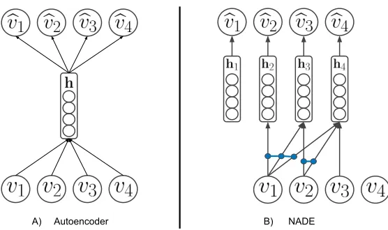
Instead of a single projection of the input vector (like for a typical autoencoder, the left part of Figure 1), the NADE model relies on a set of separate hidden layershi(v<i)that each represent the previous inputs in a latent space (right part of Figure 1). The connections between the input dimen-sionvi and each hidden layerhi(v<i)are tied as shown with the blue lines in Figure 1, allowing
the model to compute all the hidden layers for one input inO(DH). The parameters{b,c,W,V}
are learned by minimizing the average negative log-likelihood using stochastic gradient descent.
2.2 From NADE to DocNADE
A) Autoencoder B) NADE
Figure 1: A) Typical structure for an autoencoder. B) Illustration of NADE. Colored lines iden-tify the connections that share parameters andbvi is a shorthand for the autoregressive
conditionalp(vi|v<i). The observationsviare binary.
co-occurrence of words within documents and can be considered as modeling hidden topics. This is called topic modeling (Steyvers and Griffiths, 2007), where a topic model gives a mathematical representation of a document in the form of a vector (of real values). In our case each element of the vector is a neuron of the hidden layer and can be associated to a hidden subject where its value would represent how much that subject is part of the text. This representation can be seen as a composition of the subjects.
To represent a document for DocNADE, we transform a bag-of-words into a sequence v of arbitrary sizeD. Each element ofvcorresponds to a multinomial observation (representing a word) over a fixed vocabulary of sizeV:
v= [v1, v2, ... , vD], vi ∈ {1,2, ... , V}. (5)
Thereforevi represents the index in the vocabulary of thei-th word of the document. For now,
we assume that an ordering of the words is given, but we will discuss the general case of orderless bags-of-words in the next Section (2.2.1) and show that we can simply use a random order for the words during training.
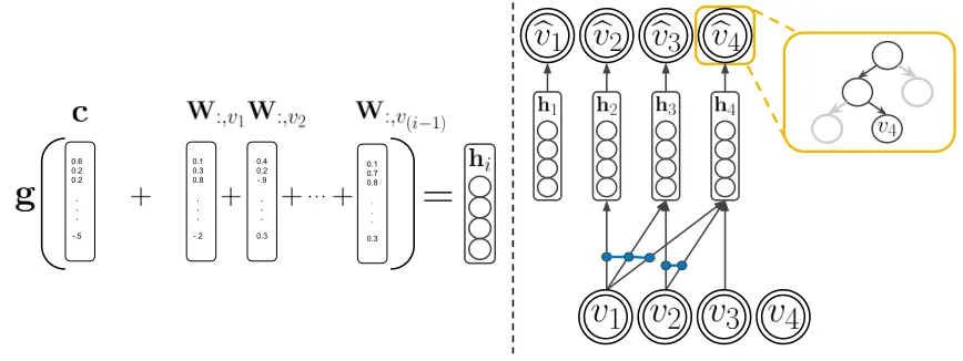
The DocNADE model uses a word representation matrix W ∈ RH×V , where each column
W:,viof the matrix is a vector representing one of the words in the vocabulary (see Figure 2). This
matrix makes the connection possible between the indexviof a word and its embedding.
The main approach taken by DocNADE is similar to NADE, but differs significantly in the design of parameter tying. The probability of a documentvis estimated using the probability chain rule, but the architecture is modified to cope with large vocabularies. Each word observationviof
0.1 0.3 0.8 . . . -.2 0.4 0.2 -.9 . . . 0.3 0.1 0.7 0.8 . . . 0.3
the a dog
Figure 2: Word representation matrixW, where each column of the matrix is a vector representing a word of the vocabulary.
This hidden layer is computed as follows:
hi(v<i) =g c+ X
k<i
W:,vk !
, (6)
where each column of the matrixWacts as a vector of sizeHthat represents a word. The embed-ding of theithword in the document is thus the column of indexviin the matrixW.
0.1 0.3 0.8 . . . -.2 0.4 0.2 -.9 . . . 0.3 0.1 0.7 0.8 . . . 0.3 0.6 0.2 0.2 . . . -.5
Figure 3: (Left) Representation of the computation of a hidden layerhi, functiong(·)can be any
activation function. (Right) Illustration of DocNADE. Connections between each multi-nomial observationviand hidden units are also shared, and each conditionalp(vi|v<i)is
decomposed into a tree of binary logistic regressions.
Notice that by sharing the word representation matrix across positions in the document, each hidden layer hi(v<i) is in fact independent of the order of the words within v<i. We made the
its importance compared to the other words does not deteriorate over time. This phenomenon can be observed in the left part of Figure 3. With this illustration we see that if we swap the first word v1with the last onevi−1we would obtain the same hidden representationhi.
It is also worth noticing that we can compute hi+1 recursively by keeping track of the pre-activation of the previous hidden layerhias follows:
hi+1(v<i+1) =g
W:,vi+ c+ X
k<i
W:,vk
| {z }
Precomputed forhi(v<i)
(7)
The weight sharing between the hidden layers enables us to compute all the hidden layershi(v<i)
for a document inO(DH).
To compute the probability of a full documentp(v), we need to estimate all conditional proba-bilitiesp(vi|v<i). A straightforward solution would be to compute eachp(vi|v<i)using a softmax
layer with a shared weight matrix and bias with each of the hidden layershi. However, the
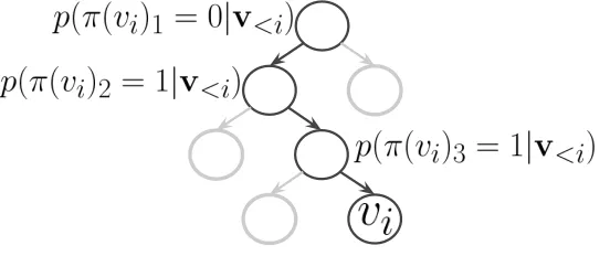
com-putational cost of this approach is prohibitive, as it scales linearly with the vocabulary size.1 To overcome this issue, we represent a distribution over the vocabulary by a probabilistic binary tree, where the leaves correspond to the words. This approach is widely used in the field of neural probabilistic language models (Morin and Bengio, 2005; Mnih and Hinton, 2009). Each word is represented by a path in the tree, going from the root to the leaf associated to that word. A binary logistic regression unit is associated to each node in the tree and gives the probability of the binary choice, going left or right. A word probability can therefore be estimated by the path’s probability in this tree, resulting in a complexity inO(logV)for a balanced tree. In our experiments, we used a randomly generated full binary tree withV leaves, each assigned to a unique word in the vocabulary.
Figure 4: Path of the wordvi in a binary tree. We compute the probability of the left/right choice
(0/1) for each node of the path.
More formally, let’s denote byl(vi)the sequence of nodes composing the path, from the root of the tree to the leaf corresponding to the wordvi. Then,π(vi)is the sequence of left/right decisions
of the nodes inl(vi). For example, the root of the tree is always the first elementl(vi)1and the value
π(vi)1 will be 0 if the word is in the left sub-tree and 1 if it is in the right sub-tree (see figure 4). The matrixVstores by row the weights associated to each logistic classifier. There is one logistic classifier per node in the tree, but only a fraction of them is used for each word. LetVl(vi)m,:and
bl(vi)mbe the weights and bias of the logistic unit associated with the noden(vi)m. The probability
p(vi|v<i)given the tree and the hidden layerhi(v<i)is computed by the following formulas:
p(vi=w|v<i) =
|π(vi)| Y
m=1
p(π(vi)m =π(w)m|v<i), with (8)
p(π(vi)m= 1|v<i) = sigm bl(vi)m+Vl(vi)m,:·hi(v<i)
. (9)
This hierarchical architecture allows us to efficiently compute the probability of each word in a document and therefore the probability of the whole document with the probability chain rule (see Equation 2). As in the NADE model, the parameters of the model {b,c,W,V} are learnt by minimizing the negative log-likelihood using stochastic gradient descent.
Since there is log(V) logistic regression units for a word (one per node), each of them has a time complexity ofO(H), the complexity of computing the probability for a document ofDwords is inO(log(V)DH).
For using DocNADE to extract features from a complete document, we propose to use
h(v) =hD+1(v<D+1) =g c+
D X
k=1 W:,vk
!
(10)
which would be the hidden layer computed to obtain the conditional probability of a hypothetical
(D+ 1)-th word appearing in the document. In other words, h(v)is the representation of all the words in the document. Notice that we do not average the document representation to become invariant to document length. Averaging did not result in any performance improvement in our preliminary experiments. We conjecture that it is because every word count ni in the data was
replaced bylog(1 +ni), which reduces the variability of the input values and makes the model more invariant to the document length. However, averaging sometimes is useful, such as for the language model approach (see Section 4).
Algorithm 1 gives the pseudo-code for computing the negative log-likelihood cost used during training and the hidden layer used for representing the whole document under DocNADE.
2.2.1 TRAINING FROM BAG-OF-WORDS COUNTS
So far, we have assumed that the ordering of the words in the document is known. However, a document often takes the form of word-count vectors in which the original word order, required for specifying the sequence of conditionalsp(vi|v<i), has been lost.
It is however still possible to successfully train a DocNADE despite the absence of this infor-mation. The idea is to assume that each observed documentvwas generated by initially sampling aseeddocumentvefrom DocNADE, whose words were then shuffled using a randomly generated
ordering to produce v. With this approach, we can express the probability distribution of v by computing the marginal over all possible seed document:
p(v) = X e
v∈V(v)
p(v,ev) = X
e
v∈V(v)
Algorithm 1 Computing of the cost for training and the hidden layer for representing an entire document (DocNADE model)
Input: Multinomial observationv a←c
N LL←0
Fori= 1toDDo
hi←g(a)
p(vi)←1
Form= 1to|π(vi)|Do
p(π(vi)m= 1|v<i)←sigm bl(vi)m+Vl(vi)m,:·hi(v<i)
p(vi)←p(vi) (p(π(vi)m= 1|v<i)π(vi)m+ (1−p(π(vi)m = 1|v<i)1−π(vi)m)) End for
N LL←N LL−logp(vi)
a←a+W:,vi End for
hf inal ←g(a) Return N LL, hf inal
wherep(ve)is modeled by DocNADE.evis the same as the observed documentvbut with a different
(random) word sequence order, andV(v)is the set of all the documentsvethat has the same word
countn(v) = n(ve). With the assumption of orderings being uniformly sampled, we can replace p(v|ve)with |V(1v)| giving us:
p(v) = X e
v∈V(v)
1
|V(v)|p(ve) = 1
|V(v)| X
e
v∈V(v)
p(ev). (12)
In practice, one approach to training the DocNADE model over ev is to artificially generate
ordered documents by uniformly sampling words, without replacement, from the bags-of-words in the dataset. This would be equivalent to taking each original document and shuffling the order of its words. This approach can be shown to minimize a stochastic upper bound on the true negative log-likelihood of documents. As we will see, experiments show that convincing performance could still be reached.
The goal with DocNADE is to have a simple, powerful, fast way to train model that can also be used with data that have lost the information about ordering. We want to learn topic-level semantics, where the order of the words is less important than the existence of words is, instead of learning syntax, where the order of the words is more important. In this context, it makes no sense to apply an RNN-like model on randomly shuffled words, since there’s no position varying information to model.
3. Deep Document NADE
The single hidden layer version of DocNADE already achieves very competitive performance for topic modeling (Larochelle and Lauly, 2012). Extending it to a deep architecture with multiple hidden layer could however enable better performance, as suggested by the recent and impressive success of deep neural networks. Unfortunately, deriving a deep version of DocNADE cannot be achieved solely by adding hidden layers to the definition of the conditionals p(vi|v<i). Indeed,
computingp(v) requires computing each p(vi|v<i) conditional (one for each word), and it is no
longer possible to use Equation 7 to compute the sequence of all hidden layers in O(DH) when there are multiple deep hidden layers.
In this Section, we describe an alternative training procedure that enables us the introduction of multiple stacked hidden layers. This procedure was first introduced by Zheng et al. (2015) to model images, which was itself borrowing from the training scheme introduced by Uria et al. (2014).
As mentioned in Section 2.2.1, DocNADE can be trained on random permutations of the words from training documents. As noticed by Uria et al. (2014), the use of many orderings during training can be seen as the instantiation of many different DocNADE models that share a single set of parameters. Thus, training DocNADE with random permutations also amounts to minimizing the negative log-likelihood averaged across all possible orderings, for each training examplev.
In the context of deep NADE models, a key observation is that training on all possible orderings implies that for a given contextv<i, we encourage the model to be equally good at predicting any
of the remaining words appearing next. Thus, we redesign the training algorithm such that, instead of sampling a complete ordering of all words for each update, we instead sample a single context v<i and perform an update of the conditionals using that context. This is done as follows. For a
given document, after generating vectorvby shuffling the words from the document, a split pointi is randomly drawn. From this split point we obtain two parts of the document,v<iandv≥i:
v= [v1, ... , vi−1
| {z }
v<i
, vi, ... , vD
| {z }
v≥i
]>. (13)
The vectorv<iis considered as the input and the vectorv≥icontains the targets to be predicted
by the model. Since a training update relies on the computation of a single latent representation, that ofv<i for the drawn value ofi, deeper hidden layers can be added at a reasonable increase in
. . .
. . . . . . . . .
1
. . .
0.1 0.3 0.8
. . .
-.2 0.4 0.2 -.9
. . .
0.3
0.1 0.7 0.8
. . .
0.3 0.6
0.2 0.2
. . .
-.5
1
1 2
0
1
. . .
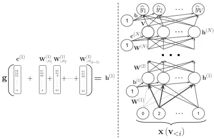
Figure 5: (Left) Representation of the computation by summation of the first hidden layer h(1), which is equivalent to multiplying the bag-of-wordsx(v<i)with the word representation
matrixW(1). (Right) Illustration of DeepDocNADE architecture.
In DeepDocNADE the conditionals p(vi|v<i) are modeled as follows. The first hidden layer
h(1)(v<i)represents the conditioning contextv<ias in the single hidden layer DocNADE:
h(1)(v<i) =g c(1)+ X
k<i
W(1):,vk
!
=gc(1)+W(1)·x(v<i)
(14)
wherex(v<i)is the histogram vector representation (bag-of-words) of the word sequencev<i, and
the exponent is used as an index over the hidden layers and its parameters, with(1)referring to the first layer (see Figure 5). The matrixW(1) is the word representation matrix of DeepDocNADE. Notice that like DocNADE, the first hidden layer h(1)(v<i) of DeepDocNADE is independent of the order of the words withinv<i. We can now easily add new hidden layers as in a regular deep
feed-forward neural network:
h(n)(v<i) =g(c(n)+W(n)·h(n−1)(v<i)), (15)
forn= 2, . . . , N, whereN is the total number of hidden layers. From the last hidden layerh(N), we compute the conditionalp(vi =w|v<i), for any wordw:
b
yw =p(vi=w|v<i) = softmax(Vw,:·h(N)(v<i) +bw), (16)
b
where V ∈ RV×H(N)
is the output parameter matrix and b the bias vector. The notation byis a
vector that represents the probability of all the vocabulary words computed at once. Each element of the vector, yˆ1 to yˆV, represents one of the words in the vocabulary. We use yˆw to make the
connection withvi =w(the index of the wordwat timei).
Finally, the loss function used to update the model for the given contextv<iis:
L(v) = Dv
Dv−i+ 1
X
w∈v≥i
−logp(vi =w|v<i), (18)
whereDvis the number of words inv, and the summation iterates over all the wordswpresent in v≥i. Thus, as described earlier, the model predicts each remaining word after the splitting position
i as if it was actually at position i. The factor in front of the summation comes from the fact that the complete log-likelihood would containDvlog-conditionals and that we are averaging over Dv −i+ 1 possible choices for the word at position i. For a more detailed presentation, see Zheng et al. (2015). The average loss function of Equation 18 is optimized with stochastic gradient descent.2
Note that to compute the probability p(vi = w|v<i), a probabilistic tree could again be used.
However, since all probabilities needed for an update are based on a single context v<i, a single
softmax layer is sufficient to compute all necessary quantities. Therefore the computational burden of a conventional softmax is not as prohibitive as for DocNADE, especially with an efficient im-plementation on the GPU. For this reason, in our experiments with DeepDocNADE we opted for a regular softmax.
4. DocNADE Language Model
While topic models such as DocNADE can be useful in learning topic representations of documents, they are very poor models of language. In DocNADE, this is due to the fact that, when assigning a probability to the next word in a sentence, it ignores the order in which the previously observed words appeared. Yet, this ordering of words conveys a lot of information regarding a syntactic role of the next word or the finer semantics within the sentence. In fact, most of that information is predictable from the last few words, which is why N-gram language models remain a dominating approach to language modeling.
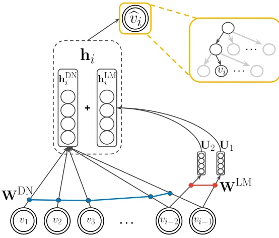
In this Section, we propose a new model that extends DocNADE to mitigate the influence of both short and long term dependencies in a single model, which we refer to as the DocNADE language model or DocNADE-LM. The solution we propose enhances the bag-of-words representation with the explicit inclusion ofn-gram dependencies.
Figure 6 depicts the overall architecture. This model can be seen as an extension of the sem-inal work on neural language models by Bengio et al. (2003) that includes the representation of a document’s larger context. It can also be seen as a neural extension of the cache-based language model introduced in (Kuhn and Mori, 1990), where then-gram probability is interpolated with the
2. A document is usually represented as bag-of-words. Generating a word vectorvfrom its bag-of-words, shuffling
the word count vectorv, splitting it, and then regenerating the histogramx(v<i)andx(v≥i)is unfortunately fairly
inefficient for processing samples in a mini-batch fashion. Hence, in practice, we split the original histogramx(v)
. . . +
. . . . . .
Figure 6: Illustration of the conditionalp(vi|v<i)in a trigram NADE language model. Compared to
DocNADE, this model incorporates the architecture of a neural language model, that first maps previous words (2 for a trigram model) to vectors using an embedding matrixWLM before connecting them to the hidden layer using regular (untied) parameter matrices (U1, U2 for a trigram). In our experiments, each conditionalp(vi|v<i)exploits decomposed
into a tree of logistic regressions, the hierarchical softmax.
word distribution observed in a dynamic cache. This cache of a fixed size keeps track of previously observed words to include long term dependencies in the prediction and preserve semantic consis-tency beyond the scope of the n-gram. The DocNADE language model maintains an unbounded cache and defines a proper, jointly trained solution to mitigate these two kinds (long and short) of dependencies.
As in DocNADE, a document vis modeled as a sequence of multinomial observations. The sequence size is arbitrary and this time the order is important, each elementvi consists of thei-th
word of the sequence and represent an index in a vocabulary of sizeV. The conditional probability of a word given its history p(vi|v<i) is now expressed as a smooth function of a hidden layer
hi(v<i) used to predict word vi. The peculiarity of the DocNADE language model lies in the
definition of this hidden layer, which now includes two terms:
hi(v<i) =g(b+hDNi (v<i) +hLMi (v<i)). (19)
The first term borrows from the DocNADE model by aggregating embeddings for all the previous words in the history:
hDNi (v<i) = 1
i−1 X
k<i
WDN:,vk , (20)
representation can become invariant to the document’s length. The hidden representationhDNi (v<i)
models the semantic aspects of the text that have been observed so far. As we explained earlier for DocNADE, the order of the words withinv<i is not modeled. The hidden layerhDNi (v<i)can be
seen as a context representation of the past where the influence of a word relative to other words does not diminish over time.
The second contribution derives from a neuraln-gram language model as follows:
hLMi (v<i) = n−1
X
k=1
Uk·WLM:,vi−k . (21)
In this formula, the history for the wordvi is restricted to the n−1preceding words, following
the commonn-gram assumption. The termhLMi hence represents the continuous representation of thesen−1 words, in which word embeddings are linearly transformed by the ordered matrices U1,U2, ...,Un−1. Moreover, b gathers the bias terms for the hidden layer. In this model, two sets of word embeddings are defined, WDN andWLM, which are respectively associated to the DocNADE and neural language model parts. For simplicity, we assume both are of the same size H.
Given hidden layerhi(v<i), conditional probabilitiesp(vi|v<i)can be estimated, and thusp(v).
For the aforementioned reason explained in DocNADE, the output layer is structured as a proba-bilistic tree for efficient computations. Specifically, we decided to use a variation of the probaproba-bilistic binary tree, known as a hierarchical softmax layer. In this case, instead of having binary nodes with multiple levels in the tree, we have only two levels where all words have their leaf at level two and each node is a multiclass (i.e. softmax) logistic regression with roughly√V classes (one for each children). Computing probabilities in such a structured layer can be done using only two matrix multiplications, which can be efficiently computed on the GPU.
With a hidden layer of sizeH, the complexity of computing the softmax at one node isO(H√V). If we haveDwords in a given document, the complexity of computing all necessary probabilities from the hidden layers is thusO(DH√V). It also requiresO(DH)computations to compute the hidden representations for the DocNADE part andO(nH2)for the language model part. The full complexity for computingp(v)and the updates for the parameters is thusO(DH√V+DH+nH2). Once again, the loss function of the model is the negative log-likelihood, and we minimize it by using stochastic gradient descent over documents, to learn the values of the parameters
{b,c,V,WLM,WDN,U1, ...,Un}.
5. Related Work
As NADE was inspired by the RBM, DocNADE can be seen as related to the Replicated Softmax model (Salakhutdinov and Hinton, 2009), an extension of the RBM to document modeling. Here, we describe in more detail the Replicated Softmax, along with its relationship with DocNADE.
Much like the RBM, the Replicated Softmax models observations using a latent, stochastic binary layerh. Here, the observation is a documentvand interacts with the hidden layerhthrough an energy function similar to RBM’s:
E(v,h) =−Dc>h+ D X
i=1
−h>W:,vi−bvi =−Dc
>
Figure 7: Replicated Softmax model. Each multinomial observation vi is a word. Connections
between each multinomial observationvi and hidden units are shared.
where n(v) is a bag-of-words vector of size V (the size of the vocabulary) containing the word count of each word in the vocabulary for documentv. his a stochastic, binary hidden layer vector, andW:,vi is thevi-th column vector of matrixW. candbare the bias vectors for the visible and
the hidden layers. We see here that the largervis, the bigger the number of terms in the sum over iis, resulting in a high energy value. For this reason, the hidden bias termc>h is multiplied by D, to be commensurate with the contribution of the visible layer.. We can see also that connection parameters are shared across different positionsiinv, as illustrated in Figure 7.
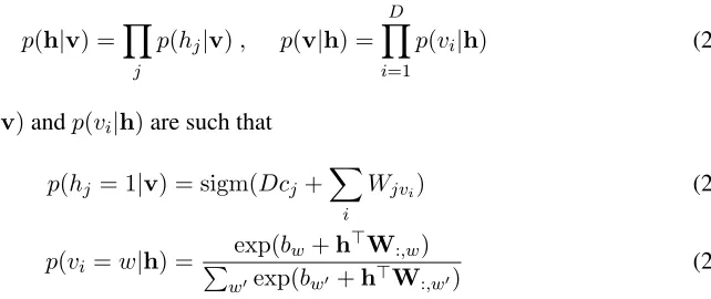
The conditional probabilities of the hidden and the visible layer factorize as in the RBM, in the following way:
p(h|v) =Y j
p(hj|v), p(v|h) = D Y
i=1
p(vi|h) (23)
where the factorsp(hj|v)andp(vi|h)are such that
p(hj = 1|v) = sigm(Dcj + X
i
Wjvi) (24)
p(vi=w|h) =
exp(bw+h>W:,w)
P
w0exp(bw0+h>W:,w0) (25) The normalized exponential part inp(vi =w|h)is simply the softmax function. To train this model,
we minimize the negative log-likelihood (NLL). Its gradient for a documentv(t)with respect to the parametersθ={W,c,b}is calculated as follows:
−∂logp(v
(t))
∂θ =EEh|v(t)
∂ ∂θE(v
(t),h)
−EEv,h
∂
∂θE(v,h)
. (26)
During Gibbs sampling, the Replicated Softmax model must compute and sample fromp(vi =
w|h), which requires the computation of a large softmax. Most importantly, the computation of the softmax most be repeatedK times for each update, which can be prohibitive, especially for large vocabularies. Unlike DocNADE, this softmax cannot simply be replaced by a structured softmax.
DocNADE is closely related to how the Replicated Softmax approximates, through mean-field inference, the conditionalsp(vi = w|v<i). Computing the conditionalp(vi = w|v<i) with the
Replicated Softmax is intractable. However, we could use mean-field inference to approximate the full conditionalp(vi,v>i,h|v<i)by introducing a factorized approximate distribution:
q(vi,v>i,h|v<i) = Y
k≥i
q(vk|v<i) Y
j
q(hj|v<i), (27)
where q(vk = w|v<i) = µkw(i) and q(hj = 1|v<i) = τj(i). We would find the parameters
µkw(i)andτj(i)that minimize the KL divergence betweenq(vi,v>i,h|v<i)andp(vi,v>i,h|v<i)
by applying the following message passing equations until convergence:
τj(i)←sigm
D cj+
X
k≥i V X
w0=1
Wjw0µkw0(i) +
X
k<i
Wjvk
, (28)
µkw(i)←
exp(bw+PjWjwτj(i)) P
w0exp(bw0+P
jWjw0τj(i)). (29)
withk∈ {i, . . . , D},j ∈ {1, . . . , H}andw∈ {1, . . . , V}. The conditionalp(vi =w|v<i)is then
estimated withµkw(i)for alli. We note that one iteration of mean-field (withµkw0(i)initialized to 0) in the Replicated Softmax corresponds to the conditionalp(vi =w|v<i)computed by DocNADE
with a single hidden layer and a flat softmax output layer.
In our experiment, we show that DocNADE compares favorably to Replicated Softmax.
5.1 Related work discussion
6. Topic modeling experiments
To compare the topic models, two quantitative measures are used. The first one evaluates the gen-erative ability of different models, by computing the perplexity on held-out texts. The second one compares the quality of document representations for information retrieval.
Two different datasets are used for the experiments in this Section, a small one and a relatively big one, 20 Newsgroups and RCV1-V2 (Reuters Corpus Volume I) respectively. The 20 News-groups corpus has 18,786 documents (postings) partitioned into 20 different classes (newsNews-groups). RCV1-V2 is a much bigger dataset composed of 804,414 documents (newswire stories) manually categorized into 103 classes (topics). The two datasets were preprocessed by stemming the text and removing common stop-words. The 2,000 most frequent words of the 20 Newsgroups training set and the 10,000 most frequent words of the RCV1-V2 training set were used to create the dictionary for each dataset. Also, every word countni, used to represent the number of times a word appears in
a document, was replaced withlog(1 +ni)rounded to the nearest integer, following Salakhutdinov
and Hinton (2009).
For these experiments, all the hidden representations of all the models are composed of 50 dimensional features. Early stopping on the validation set is used for avoiding overfitting and for model selection.
6.1 Generative Model Evaluation
For the generative model evaluation, we follow the experimental setup proposed by Salakhutdinov and Hinton (2009) for 20 Newsgroups and RCV1-V2 datasets. We use the exact same split for the sake of comparison. The setup consists of respectively 11,284 and 402,207 training examples for 20 Newsgroups and RCV1-V2. We randomly extract 1,000 and 10,000 documents from the training sets of 20 Newsgroups and RCV1-V2, respectively, to build a validation set. The average perplexity per word is used for comparison. This perplexity is estimated using the 50 first documents of a separate test set, as follows:
exp −1
T
X
t 1
|vt|logp(v t)
!
, (30)
whereT is the total number of examples in the test set andvtis thet-th test document.3
Table 1 presents the perplexities per word results for 20 Newsgroups and RCV1-V2. We com-pare 5 different models: the Latent Dirichlet Allocation (LDA) (Blei et al., 2003), the Replicated Softmax, the recently proposed fast Deep AutoRegressive Networks (fDARN) (Mnih and Gregor, 2014), DocNADE and DeepDocNADE (DeepDN in the table). Each model uses 50 latent topics (size of the representation of a document). For the experiments with DeepDocNADE, we provide the performance when using 1, 2, and 3 hidden layers. As shown in Table 1, DeepDocNADE re-sults in the best generative performances. Our best DeepDocNADE models were trained with the Adam optimizer (Kingma and Ba, 2014) and withtanhactivation function. The hyper-parameters of Adam were selected on the validation set.
Dataset LDA Replicated fDARN DocNADE DeepDN DeepDN DeepDN
Softmax (1layer) (2layer) (3layer)
20 News 1091 953 917 896 835 877 923
RCV1-v2 1437 988 724 742 579 552 539
Table 1: Test perplexity per word for models with a document representation of size 50 (50 topics). The results for LDA and Replicated Softmax were taken from Salakhutdinov and Hinton (2009).
0 50 100 150 200 250 300 Number of Ensembles
800 850 900 950 1000 1050
Perplexity
DeepDocNADE(1 hidden layers) DeepDocNADE(2 hidden layers) DeepDocNADE(3 hidden layers)
0 50 100 150 200 250 300 Number of Ensembles
520 540 560 580 600 620 640
Perplexity
DeepDocNADE(1 hidden layers) DeepDocNADE(2 hidden layers) DeepDocNADE(3 hidden layers)
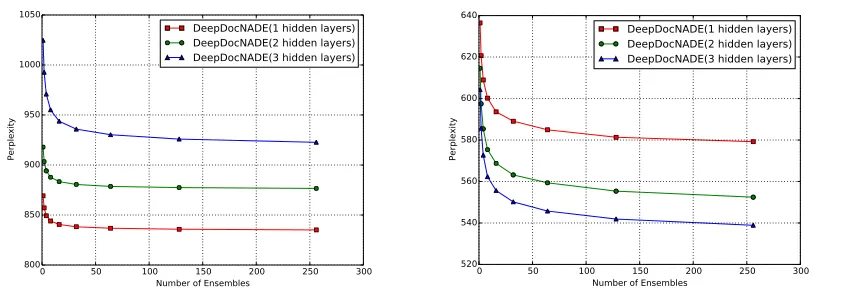
Figure 8: Perplexity obtained with different numbers of word orderingsmfor 20 Newsgroups on the left and RCV1-V2 on the right.
Furthermore, following Uria et al. (2014), an ensemble approach is used to compute the proba-bility of documents, where each component of the ensembles are the same DeepDocNADE model evaluated on a different word ordering. The perplexity withM ensembles is then
exp −1
T
X
t 1
|vt|log 1
M
X
m
p(v(t,m)) !!
, (31)
whereTis the total number of examples,Mis the number of ensembles (word orderings) andv(t,m) denotes them-th word ordering for thet-th document. We tryM ={1,2,4,16,32,64,128,256}, with the results in Table 1 usingM = 256. For the 20 Newsgroups dataset, adding more hidden layers to DeepDocNADE fails to further improve the performance. We hypothesize that the rel-atively small size of this dataset makes it hard to successfully train a deep model. However, the opposite is observed on the RCV1-V2 dataset, which is more than an order of magnitude larger than 20 Newsgroups. In this case, DeepDocNADE outperforms fDARN and DocNADE, with a relative perplexity reduction of 20%, 24% and 26% with respectively 1,2 and 3 hidden layers.
To illustrate the impact of M on the performance of DeepDocNADE, Figure 8 shows the per-plexity on both datasets using the different values forM that we tried. We can observe that beyond
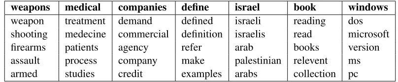
weapons medical companies define israel book windows
weapon treatment demand defined israeli reading dos shooting medecine commercial definition israelis read microsoft firearms patients agency refer arab books version assault process company make palestinian relevent ms armed studies credit examples arabs collection pc
Table 2: The five nearest neighbors in the word representation space learned by DocNADE.
6.2 Document Retrieval Evaluation
A document retrieval evaluation task was also used to evaluate the quality of the document repre-sentation learned by each model. As in the previous Section, the datasets under consideration are 20 Newsgroups and RCV1-V2. The experimental setup is the same for the 20 Newsgroups dataset, while for the RCV1-V2 dataset, we reproduce the same setup as the one used by Srivastava et al. (2013). The training set contains 794,414 examples and 10,000 examples constituted the test set.
For DocNADE and DeepDocNADE, the representation of a document is obtained simply by computing the top-most hidden layer (Equation 10) when feeding all the words of a document as input.
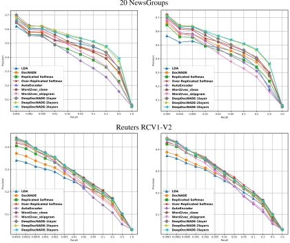
The retrieval task follows the setup by Srivastava et al. (2013). The documents in the training and validation sets are used as the database for retrieval, while the test set is used as the query set. The similarity between a query and all examples in the database is computed using the cosine similarity between their vector representations. For each query, documents in the database are then ranked according to this similarity, and precision/recall (PR) curves are computed, by comparing the label of the query documents with those of the database documents. Since documents often have multiple labels (specifically those in RCV1-V2), the PR curves for each of its labels are computed individually and then averaged for each query. Finally, we report the global average of these (query-averaged) curves to compare models against each other. Training and model selection is otherwise performed as done in the generative modeling evaluation.
As shown in Figure 9, DeepDocNADE always yields very competitive results, on both datasets, and outperforming the other models in most cases. Specifically, for the 20 Newsgroups dataset, DeepDocNADE with 2 and 3 hidden layers always perform better than the other methods. Deep-DocNADE with 1 hidden layer also performs better than the other baselines when retrieving the top few documents ( e.g. when recall is smaller than 0.2).
6.3 Qualitative Inspection of Learned Representations
In this Section, we want to assess if the DocNADE approach for topic modeling can capture mean-ingful semantic properties of texts.
First, one way to explore the semantic properties of trained models is through their learned word embeddings. Each of the columns of the matrixW represents a wordwwhereW:,w is the vector
20 NewsGroups
0.001 0.002 0.005 0.01 0.02 0.05 0.1 0.2 0.5 1.0 Recall 0.1 0.2 0.3 0.4 0.5 0.6 0.7 Precision LDA DocNADE Replicated Softmax Over-Replicated Softmax AutoEncoder Word2vec_cbow Word2vec_skipgram DeepDocNADE-1layer DeepDocNADE-2layers DeepDocNADE-3layers
0.001 0.002 0.005 0.01 0.02 0.05 0.1 0.2 0.5 1.0 Recall 0.1 0.2 0.3 0.4 0.5 0.6 0.7 Precision LDA DocNADE Replicated Softmax Over-Replicated Softmax AutoEncoder Word2vec_cbow Word2vec_skipgram DeepDocNADE-1layer DeepDocNADE-2layers DeepDocNADE-3layers Reuters RCV1-V2
0.0001 0.0002 0.0005 0.001 0.002 0.005 0.01 0.02 0.05 0.1 0.2 0.5 1.0 Recall 0.1 0.2 0.3 0.4 Precision LDA DocNADE Replicated Softmax Over-Replicated Softmax AutoEncoder Word2vec_cbow Word2vec_skipgram DeepDocNADE-1layer DeepDocNADE-2layers DeepDocNADE-3layers
0.0001 0.0002 0.0005 0.001 0.002 0.005 0.01 0.02 0.05 0.1 0.2 0.5 1.0 Recall 0.1 0.2 0.3 0.4 Precision LDA DocNADE Replicated Softmax Over-Replicated Softmax AutoEncoder Word2vec_cbow Word2vec_skipgram DeepDocNADE-1layer DeepDocNADE-2layers DeepDocNADE-3layers
Figure 9: Precision-Recall curves for document retrieval task. On the left are the results using a hidden layer size of 128, while the plots on the right are for a size of 512.
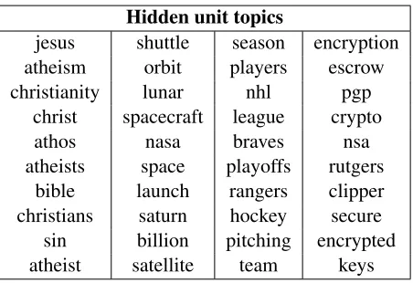
We have also attempted to measure whether the hidden units of the first hidden layer of Doc-NADE and DeepDocDoc-NADE models modeled distinct topics. Understanding the function repre-sented by hidden units in neural networks is not a trivial affair, but we considered the following simple approach. For a given hidden unit, its connections to words are interpreted as the importance of the word for the associated topic. We thus select the words having the strongest positive con-nections for a hidden unit, i.e. for thei-th hidden unit we chose the wordswthat have the highest connection valuesWi,w.
With this approach, fifty topics were obtained from a DocNADE model (with the sigmoid acti-vation function) trained on 20 Newsgroups. Four of the fifty topics are shown in Table 3 and can be readily interpreted as topics representing: religion, space, sports and security. Note that those four topics are actual (sub)categories in 20 Newsgroups.
That said, we have had less success understanding the topics extracted when using the tanh
Hidden unit topics
jesus shuttle season encryption atheism orbit players escrow christianity lunar nhl pgp
christ spacecraft league crypto
athos nasa braves nsa
atheists space playoffs rutgers bible launch rangers clipper christians saturn hockey secure sin billion pitching encrypted atheist satellite team keys
Table 3: Illustration of some topics learned by DocNADE. A topiciis visualized by picking the 10 wordswwith strongest connectionWiw.
representation that does not align its dimensions with concepts that are easily interpretable, even though it is clearly capturing well the statistics of documents.
7. Language Modeling Experiments
In this Section, we test whether our proposed approach to incorporating a DocNADE component to a neural language model can improve the performance of a neural language model. Specifically, we considered treating a text corpus as a sequence of documents. We used the APNews dataset, as pro-vided by Mnih and Hinton (2009). Unfortunately, information about the original segmentation into documents of the corpus was not available in the data as provided by Mnih and Hinton (2009), thus we simulated the presence of documents by grouping one or more adjacent sentences, for training and evaluating DocNADE-LM, making sure the generated documents were non-overlapping. This approach still allows us to test whether DocNADE-LM is able to effectively leverage the larger context of words in making its predictions.
Since language models are generative models, the perplexity measured on some held-out texts is widely used for evaluation. Following Mnih and Hinton (2007) and Mnih and Hinton (2009), we use the APNews dataset containing Associated Press news stories from 1995 and 1996. The dataset is again split into training, validation and test sets with respectively 633,143, 43,702 and 44,601 sentences. The vocabulary is composed of 17,964 words.
For these experiments, all the hidden representations of all the models are composed of 100 dimensional features. Early stopping on the validation set is used for avoiding overfitting and for model selection. The perplexity scores of Table 4 are computed on the test set.
The LM model in Table 4 corresponds to a regular neural (feed-forward) network language model. It is equivalent to using only the language model part of DocNADE-LM. These results are meant to measure whether the DocNADE part of DocNADE-LM indeed improves performances.
Models Number of grouped sentences Perplexity
KN6 1 123.5
LBL 1 117.0
HLBL 1 112.1
LSTM 1 116.26
GRU 1 109.42
LM 1 119.78
DocNADE-LM 1 111.93
DocNADE-LM 2 110.9
DocNADE-LM 3 109.8
DocNADE-LM 4 109.78
DocNADE-LM 5 109.22
Table 4: Test perplexity per word for models with 100 topics. The results for HLBL and LBL were taken from Mnih and Hinton (2009).
and Hinton (2009) also proposed an adaptive approach to learning a structured softmax layer, thus we also compare against their best approach. All the aforementioned baselines are 6-gram models, taking in consideration the five previous words to predict the next one. We also compare with a more traditional 6-gram model using Kneser-Ney smoothing, taken from Mnih and Hinton (2007). Finally we compare our results against recurrent language model using ether LSTM from Graves (2013) or GRU from Cho et al. (2014). These models are trained with stochastic gradient descent, using full backpropagation through time. They are considered as states of the art for modeling sequences.
From Table 4, we see that adding context to DocNADE-LM, by increasing the size of the multi-sentence segments, improves the performance of the model (compared to LM) and also surpasses the performance of the most competitive alternatives.
7.1 Qualitative Inspection of Learned Representations
In this Section we explore the semantic properties of texts learned by the DocNADE-LM model. Interestingly, we can examine the two different components (DN and LM) separately. Because the DocNADE part and the language modeling part of the model each have their own word matrix, WDNandWLMrespectively, we can compare their contribution through these learned embeddings. As explained in the previous Section, each of the columns of the matrices represents a wordwwhere WDN
:,w andWLM:,w are two different vector representations of the same wordw.
weapons medical companies define israel book windows
security doctor industry spoken israeli story yards humanitarian health corp to palestinian novel rubber terrorists medicine firms think of jerusalem author piled
deployment physicians products of lebanon joke fire department diplomats treatment company bottom line palestinians writers shell
Table 5: The five nearest neighbors in the word representation space learned by the DocNADE part of the DocNADE-LM model.
weapons medical companies define israel book windows
systems special countries talk about china film houses aircraft japanese nations place russia service room
drugs bank states destroy cuba program vehicle
equipment media americans show north korea movie restaurant services political parties over lebanon information car
Table 6: The five nearest neighbors in the word representation space learned by the language model part of the DocNADE-LM model.
8. Conclusion
References
Yoshua Bengio, R´ejean Ducharme, Pascal Vincent, and Christian Janvin. A neural probabilistic language model. The Journal of Machine Learning Research, 3:1137–1155, 2003.
David M. Blei, Andrew Y. Ng, and Michael I. Jordan. Latent Dirichlet Allocation. Journal of
Machine Learning Research, 3(4-5):993–1022, 2003.
Jonathan Chang, Jordan Boyd-Graber, Sean Gerrish, Chong Wang, and David Blei. Reading Tea Leaves: How Humans Interpret Topic Models. In Advances in Neural Information Processing
Systems 22 (NIPS 2009), pages 288–296, 2009.
Kyunghyun Cho, Bart Van Merri¨enboer, Caglar Gulcehre, Dzmitry Bahdanau, Fethi Bougares, Hol-ger Schwenk, and Yoshua Bengio. Learning phrase representations using rnn encoder-decoder for statistical machine translation. arXiv preprint arXiv:1406.1078, 2014.
Alex Graves. Generating sequences with recurrent neural networks. arXiv preprint arXiv:1308.0850, 2013.
Geoffrey E. Hinton. Training products of experts by minimizing contrastive divergence. Neural
Computation, 14:1771–1800, 2002.
Diederik Kingma and Jimmy Ba. Adam: A method for stochastic optimization. arXiv preprint arXiv:1412.6980, 2014.
R. Kuhn and R. De Mori. A cache-based natural language model for speech recognition. IEEE Transactions on Pattern Analysis and Machine Intelligence, 12(6):570–583, june 1990.
Hugo Larochelle and Stanislas Lauly. A neural autoregressive topic model. InAdvances in Neural
Information Processing Systems, pages 2708–2716, 2012.
Hugo Larochelle and Ian Murray. The Neural Autoregressive Distribution Estimator. InProceedings of the 14th International Conference on Artificial Intelligence and Statistics (AISTATS 2011), volume 15, pages 29–37, Ft. Lauderdale, USA, 2011. JMLR W&CP.
Quoc Le and Tomas Mikolov. Distributed representations of sentences and documents. In
Proceed-ings of the 31st International Conference on Machine Learning (ICML-14), pages 1188–1196,
2014.
Greg Corrado Jeffrey Dean Mikolov, Kai Chen. Efficient Estimation of Word Representations in Vector Space. InWorkshop Track of the 1st International Conference on Learning Representa-tions (ICLR 2013), 2013.
Tomas Mikolov, Kai Chen, Greg Corrado, and Jeffrey Dean. Efficient estimation of word represen-tations in vector space. arXiv preprint arXiv:1301.3781, 2013.
Andriy Mnih and Geoffrey Hinton. Three new graphical models for statistical language modelling. InProceedings of the 24th international conference on Machine learning, pages 641–648. ACM, 2007.
Andriy Mnih and Geoffrey E Hinton. A Scalable Hierarchical Distributed Language Model. In
Advances in Neural Information Processing Systems 21 (NIPS 2008), pages 1081–1088, 2009.
Frederic Morin and Yoshua Bengio. Hierarchical Probabilistic Neural Network Language Model. In Proceedings of the 10th International Workshop on Artificial Intelligence and Statistics (AISTATS 2005), pages 246–252. Society for Artificial Intelligence and Statistics, 2005.
Ruslan Salakhutdinov and Geoffrey Hinton. Replicated Softmax: an Undirected Topic Model. In
Advances in Neural Information Processing Systems 22 (NIPS 2009), pages 1607–1614, 2009.
Nitish Srivastava, Ruslan R Salakhutdinov, and Geoffrey E Hinton. Modeling documents with deep boltzmann machines. arXiv preprint arXiv:1309.6865, 2013.
Mark Steyvers and Tom Griffiths. Probabilistic topic models.Handbook of latent semantic analysis, 427(7):424–440, 2007.
Benigno Uria, Iain Murray, and Hugo Larochelle. A deep and tractable density estimator. JMLR: W&CP, 32(1):467–475, 2014.