Online Bayesian Passive-Aggressive Learning
∗Tianlin Shi [email protected]
Institute for Interdisciplinary Information Sciences Tsinghua University
Beijing, 100084 China
Jun Zhu [email protected]
State Key Lab of Intelligent Technology and Systems
Tsinghua National Lab for Information Science and Technology Department of Computer Science and Technology
Tsinghua University Beijing, 100084 China
Editor:Amir Globerson
Abstract
We present online Bayesian Passive-Aggressive (BayesPA) learning, a generic online learning framework for hierarchical Bayesian models with max-margin posterior regularization. We show that BayesPA subsumes the standard online Passive-Aggressive (PA) learning and extends naturally to incorporate latent variables for both parametric and nonparametric Bayesian inference, therefore providing great flexibility for explorative analysis. As an important example, we apply BayesPA to topic modeling and derive efficient online learning algorithms for max-margin topic models. We further develop nonparametric BayesPA topic models to infer the unknown number of topics in an online manner. Experimental results on 20newsgroups and a large Wikipedia multi-label dataset (with 1.1 millions of training documents and 0.9 million of unique terms in the vocabulary) show that our approaches significantly improve time efficiency while achieving comparable accuracy with the corresponding batch algorithms.
1. Introduction
With the fast growth of data volume and variety, it is becoming increasingly important to develop scalable machine learning algorithms, which can be categorized into two major categories — on-line/stochastic methods on a single core and parallel/distributed algorithms on multiple-cores or multiple machines. This paper focuses on online learning, a process of answering a sequence of questions (e.g., which category does a document belong to?) given knowledge of the correct an-swers (e.g., the true category labels) to previous questions. Such a process is especially suitable for the applications with streaming data. For the applications with large datasets, online learning algorithms can effectively explore data redundancy relative to the model to be learned, by repeat-edly subsampling the data; and they often lead to faster convergence to satisfactory results than the corresponding batch learning algorithms. Among the many popular algorithms, online Passive-Aggressive (PA) learning (Crammer et al., 2006) provides a generic framework of performing online
∗. Correspondence should be addressed to J. Zhu. T. Shi is now with Stanford Artificial Intelligence Laboratory (SAIL), Stanford University, Stanford, CA, 94305
c
learning for large-margin methods (e.g., SVMs), with many applications in natural language pro-cessing and text mining (McDonald et al., 2005; Chiang et al., 2008). Though enjoying strong discriminative ability that is preferable for predictive tasks, existing online PA methods are formu-lated as a point estimate problem by optimizing some deterministic objective function. This may lead to some potential shortcomings. For example, a single large-margin model could fail to capture the rich underlying structure of complex data.
On the other hand, Bayesian methods enjoy greater flexibility in describing the possible under-lying structures of complex data by incorporating a hierarchy of latent variables. Moreover, the recent progress on nonparametric Bayesian methods (Hjort, 2010; Teh et al., 2006a) further pro-vides an increasingly important framework that allows the Bayesian models to have an unbounded model complexity, e.g., an infinite number of components in a mixture model (Hjort, 2010) or an infinite number of units in a latent feature model (Ghahramani and Griffiths, 2005), and to adapt when the learning environment changes. In particular, adaptation to the changing environment is of great importance in online learning. For Bayesian models, one challenging problem is posterior inference, for which both variational and Monte Carlo methods can be too expensive to be applied to large-scale applications. To scale up Bayesian inference, much progress has been made on develop-ing stochastic variational Bayes (Hoffman et al., 2013; Mimno et al., 2012) and stochastic gradient Monte Carlo (Welling and Teh, 2011; Ahn et al., 2012) methods, which repeatedly draw samples from a given finite dataset.1To deal with the potentially unbounded streaming data, streaming varia-tional Bayes methods (Broderick et al., 2013) have been developed as a general framework, with an application to topic models for learning latent topic representations. However, due to the generative nature, Bayesian models usually does not perform as well as discriminative models in predictive tasks such as classification.
Successful attempts have been made to bring large-margin learning and Bayesian methods to-gether to solve supervised learning tasks using flexible Bayesian latent variable models. For exam-ple, maximum entropy discrimination (MED) made a significant advance in conjoining max-margin learning and Bayesian generative models, in the context of univariate prediction (Jaakkola et al., 1999) and structured output prediction (Zhu and Xing, 2009). Recently, much attention has been devoted to generalizing MED to incorporate latent variables and perform nonparametric Bayesian inference in various contexts, including topic modeling (Zhu et al., 2012), matrix factorization (Xu et al., 2013), and multi-task learning (Jebara, 2011; Zhu et al., 2014c). Regularized Bayesian infer-ence (RegBayes) (Zhu et al., 2014c) provides a unified framework for Bayesian models to perform max-margin learning, where the max-margin principle is incorporated through adding posterior constraints to an information-theoretical optimization problem. By solving this problem involving latent variables, RegBayes can uncover structures that support the supervised learning tasks. Reg-Bayes subsumes the standard Reg-Bayes’ rule and is more flexible in incorporating domain knowledge or max-margin constraints. Though flexible in discovering latent structures and powerful in dis-criminative predictions, posterior inference in such models remains a challenge. By exploring data augmentation techniques, recent progress has been made to develop efficient MCMC methods (Zhu et al., 2014b), which can also be implemented in distributed clusters (Zhu et al., 2013). However, these batch learning methods are not applicable to streaming data, and they do not explore the statistical redundancy in large-scale corpora either.
To address the above problems of both online PA on incorporating flexible latent structures and Bayesian max-margin models on scalable streaming inference, this paper presents online Bayesian Passive-Aggressive (BayesPA) learning, a general framework of performing online learning for Bayesian max-margin models. We show that online BayesPA subsumes the standard online PA when the underlying model is linear and the parameter prior is Gaussian (See Table 1 for its close relationships with streaming variational Bayes and RegBayes). We further show that one major significance of BayesPA is its natural generalization to incorporate a hierarchy of latent variables for both parametric and nonparametric Bayesian inference, therefore allowing online BayesPA to have the great flexibility of (nonparametric) Bayesian methods for explorative analysis as well as the strong discriminative ability of large-margin learning for predictive tasks. As concrete exam-ples, we apply the theory of online BayesPA to topic modeling and derive efficient online learning algorithms for max-margin supervised topic models (Zhu et al., 2012). We further develop efficient online learning algorithms for the nonparametric max-margin topic models, an extension of the non-parametric topic models (Teh et al., 2006a) for predictive tasks. Extensive empirical results on real datasets demonstrate significant improvements on time efficiency and maintenance of comparable results with corresponding batch algorithms.
The paper is structured as follows. We discuss the related work in Section 2, and review the preliminary knowledge in Section 3. Then, we move on to the detailed description of BayesPA in Section 4, and present the theoretical analysis. Section 5 presents the concrete instantiations on topic modeling, and Section 6 presents the extensions to nonparametric topic models and multi-task learning. Section 7 presents experimental results. Finally, Section 8 concludes this paper with future directions discussed.
2. Related Work
As a well-established learning paradigm, online learning is of both theoretical and practical interest. The goal of online learning is to make a sequence of decisions, such as classification and regression, and use the knowledge extracted from previous correct answers to produce decisions on incoming ones. The root of online learning could be traced back to early studies of repeated games (Hannan, 1957), where an agent dynamically makes choices with the summary of past information. The idea became popular with the advent of Perceptron algorithms (Rosenblatt, 1958), which adopt an additive update rule for the classifier weights, and its multiplicative counterpart is the Winnow algorithm (Littlestone, 1988). The class of online multiplicative algorithms was further generalized by Adaboost (Freund and Schapire, 1997) in a decision theoretic sense and is now widely applied to various fields of study (Arora et al., 2012).
The theoretical analysis of online learning typically relies on the notion ofregret, which is the average loss incurred by an adaptive online learner on streaming data versus the best achievable through a single fixed model having the hindsight of all data (Murphy, 2012). It can be shown that the notion of regret is closely related to weak duality in convex optimization, which brings online learning to the algorithmic framework of convex repeated games (Shalev-Shwartz and Singer, 2006).
Although the classical regime of online learning is based on decision theory, recently much attention has been paid to the theory and practice of online probabilistic inference in the context of Big Data. Rooted either in variational inference or Monte Carlo sampling methods, there are broadly two lines of work on the topic of online Bayesian inference. Stochastic variational infer-ence (SVI) (Hoffman et al., 2013) is a stochastic approximation algorithm for mean-field varia-tional inference. By approximating the natural gradients in maximizing the evidence lower bound with stochastic gradients sampled from data points, Hoffman et al. (2013) demonstrated scalable inference of topic models on large corpora. Mimno et al. (2012) showed the performance of SVI could be improved through structured mean-field assumptions and locally collapsed variational in-ference. SVI is also applicable to the stochastic inference of nonparametric Bayesian models, such as hierarchical Dirichlet process (Wang et al., 2011; Wang and Blei, 2012b).
There is also a large body of work on extending Monte Carlo methods to the online setting. A classic approach is sequential Monte Carlo methods (SMC) or particle filters (Doucet and Jo-hansen, 2009), which arose from the numerical estimation of state-space models. Through Rao-Blackwellized particle filters (Doucet et al., 2000), one could obtain online inference algorithms for latent Dirichlet allocation (LDA) (Canini et al., 2009), and more recently Gao et al. (2016) presented a streaming (collapsed) Gibbs sampler with better accuracy. To tackle the sparsity issues and inade-quate coverage of particles, Steinhardt and Liang (2014) leveraged “abstract particles” to represent entire regions of the sample space. Recently, Korattikara et al. (2014) introduced an approximate Metropolis-Hasting rule based on sequential hypothesis testing that allows accepting and rejecting samples using only a fraction of the data. As an alternative, Bardenet et al. (2014) proposed an adaptive sampling strategy of Metropolis-Hastings from a controlled perturbation of the target dis-tribution. With elegant use of gradient information that Metropolis-Hastings algorithms neglected, a line of work (Welling and Teh, 2011; Ahn et al., 2012; Patterson and Teh, 2013) also developed stochastic gradient methods based on Langevin dynamics.
While most online Bayesian inference methods have adopted a stochastic approximation of the posterior distribution by sub-sampling a given finite dataset, in many applications data arrives in stream so that the dataset is changing over time and its size is unknown. To relax the previous request on knowing the data size, Broderick et al. (2013) made streaming updates to the estimated posterior and demonstrated the advantage of streaming variational Bayes (SVB) over stochastic variational inference. As will be discussed in this paper, BayesPA also does not impose assumptions on the size of dataset and works on streaming data.
data. MedLDA (Zhu et al., 2012) extends MED to infer latent topical structure from data with large margin constraints on the target posteriors. Similarly, nonparametric Bayesian max-margin models have also been developed, such as infinite SVMs (iSVM) (Zhu et al., 2011) for building SVM clas-sifiers with a latent mixture structure, and infinite latent SVMs (iLSVM) (Zhu et al., 2014c) for au-tomatic discovering predictive features for SVMs. Furthermore, the idea of nonparametric Bayesian learning has been applied to link prediction (Zhu, 2012), matrix factorization (Xu et al., 2013), etc. Regularized Bayesian inference (RegBayes) (Zhu et al., 2014c) provides a unified framework for performing max-margin learning of (nonparametric) Bayesian models, where the max-margin prin-ciple was incorporated through imposing posterior constraints to a variational formulation of the standard Bayes’ rule.
Max-margin Bayesian learning in the batch mode has already been one of the common chal-lenges facing this class of models. Despite its general intractability, efficient algorithms have been proposed under different settings. One way is to solve the problem via variational inference under a mean-field (Zhu et al., 2012) or structured mean-field (Jiang et al., 2012) assumption. Recently, Zhu et al. (2014b) provided a key insight in deriving efficient Monte Carlo methods without making strict assumptions. Their technique is based on a data augmentation formulation of the expected margin loss. Based on similar techniques, fast inference algorithms have also been developed for generalized relational topic models (Chen et al., 2015), matrix factorization (Xu et al., 2013), etc. Data augmentation (DA) refers to the method of introducing augmented variables along with the observed data to make their joint distribution tractable. The technique was popularized in the statis-tics community by the well-known expectation-maximization algorithm (EM) (Dempster et al., 1977) for maximum likelihood estimation with missing data. For posterior inference, the technique is popularized by Tanner and Wong (1987) in statistics and by Swendsen and Wang (1987) for the Ising and Potts models in physics. For a broader introduction to DA methods, we refer the readers to Van Dyk and Meng (2001).
Finally, our conference version of the paper (Shi and Zhu, 2014) has introduced some prelimi-nary work, which we largely extend here.
3. Preliminaries
This section reviews the preliminary knowledge that is needed to develop online Bayesian Passive-Aggressive learning. The relationships with BayesPA will be summarized in Table 1 later.
3.1 Online Passive-Aggressive Learning
Based on a decision-theoretic view, the goal of online supervised learning is to minimize the cu-mulative loss for a certain prediction task from the sequentially arriving training samples. Online Passive-Aggressive (PA) learning (Crammer et al., 2006) achieves this goal by updating some para-metric modelw ∈ RK (e.g., the weights of a linear SVM) in an online manner with the instanta-neous losses from arriving data{xt}t≥0 (xt ∈ RK) and corresponding responses{yt}t≥0, where
Kis the number of input features. The loss`(w;xt, yt), as they consider, could be the hinge loss
following optimization problem:
min w
1
2||w−wt||
2 s.t.:`
(w;xt, yt) = 0, (1)
where k · k is the Euclidean 2-norm. Intuitively, if wt suffers no loss from the new data, i.e., `(wt;xt, yt) = 0, the algorithmpassivelyassignswt+1 =wt; otherwise, it aggressively projects wtto the feasible region of parameter vectors that attain zero loss on the new data. With provable
regret bounds, Crammer et al. (2006) showed that online PA algorithms could achieve comparable results to the optimal classifier w∗, which has the hindsight of all data. In practice, in order to account for inseparable training samples, soft margin constraints are often adopted and the resulting PA learning problem is
min w
1
2||w−wt||
2+ 2c·`
(w;xt, yt), (2)
wherec is a positive regularization parameter and the constant factor2is included for simplicity as will be clear soon. For problems (1) and (2) with samples arriving one at a time, closed-form solutions can be derived (Crammer et al., 2006). For example, for the binary hinge loss the update rule for problem (2) is wt+1 = wt+τtytxt, whereτt = min(2c,max(0, −ytw>xt)/||xt||2); and for the-insensitive loss, the update rule iswt+1 =wt+sign(yt−w>xt)τtxt, whereτt =
max(0, −ytw>xt)/||xt||2.
3.2 Streaming Variational Bayes
For Bayesian models, Bayes’ rule naturally leads to a streaming update procedure for online learn-ing. Specifically, suppose the data{xt}t≥0 are generated i.i.d. according to a distributionp(x|w) and the priorp(w)is given. Bayes’ theorem implies that the posterior distribution ofwgiven the firstTsamples (T ≥1) satisfies
p(w|{xt}Tt=0)∝p(w|{xt}Tt=0−1)p(xT|w). (3)
In other words, the posterior after observing the firstT −1 samples is treated as the prior for the incoming data point.
This natural streaming Bayes’ rule, however, is often intractable to compute, especially for com-plex models (e.g., when latent variables are present). Streaming variational Bayes (SVB) (Brod-erick et al., 2013) suggests that a variational approximation should be adopted and it practically works well. Specifically, letAbe any algorithm that calculates an approximate posteriorq(w) =
A(X, q0(w)) based on data X and prior q0(w). Then, the recursive formula for approximate streaming update is:
q(w|{xt}Tt=0) =A
xT, q(w|{xt}Tt=0−1)
.
3.3 Regularized Bayesian Inference
The decision-theoretic and Bayesian view of learning can be reciprocal. For example, it would be beneficial to combine the flexibility of Bayesian models with the discriminative power of large-margin methods. The idea of regularized Bayesian inference (RegBayes) (Zhu et al., 2014c) is to treat Bayesian inference as an optimization problem with an imposed loss function for predic-tion tasks or a regularizapredic-tion term on the target posterior distribupredic-tion in general. Mathematically, RegBayes for supervised learning can be formulated as
min
q∈P KL
h
q(w)||p0(w)
i
−Eq(w)hlogp(X|w)i+ 2c·`q(w);X,Y, (4)
where P is the probability simplex, p(X|w) is the likelihood function andKL is the Kullback-Leibler divergence.2 Note that if the loss is zero, i.e.,`(q(w);X,Y) = 0, then the optimal solution isq∗(w) ∝ p0(w)p(X|w), which is just the Bayes’ rule. However, when `(q(w);X,Y) 6= 0, RegBayes biases the inferred posterior towards discriminating the supervising side-informationY, with the parameterccontrolling the extent of regularization. If the posterior regularization term`(·)
is a convex function ofq(w)through the linear expectation operator, Zhu et al. (2014c) presented a general representation theorem to characterize the solution to problem (4). To distinguish from the posterior distribution obtained via Bayes’ rule, the solution to problem (4) is calledpost-data poste-rior(Zhu et al., 2014c). Many instantiations have been developed following the generic framework of RegBayes to demonstrate its superior performance than standard Bayesian models in various settings, such as topic modeling (Jiang et al., 2012; Zhu et al., 2014b), matrix factorization (Xu et al., 2013) and link prediction (Zhu, 2012), as well as the flexibility of performing robust Bayesian inference with noisy domain knowledge (Mei et al., 2014).
4. Bayesian Passive-Aggressive Learning
In this section, we present online Bayesian Passive-Aggressive (BayesPA) learning, a general per-spective on online max-margin Bayesian inference. Without loss of generality, we consider binary classification. The techniques can be applied to other learning tasks. We provide an extension in Section 6.2.
4.1 Online BayesPA Learning
Instead of updating a point estimate ofw, online Bayesian PA (BayesPA) sequentially infers a new post-data posterior distributionqt+1(w), either parametric or nonparametric, on the arrival of a new data point(xt, yt)by solving the following optimization problem:
min
q(w)∈Ft
KLhq(w)||qt(w)
i
−Eq(w)hlogp(xt|w)
i
s.t.: `
q(w);xt, yt
= 0,
(5)
2. We assume that the model spaceW is a complete separable metric space endowed with its Borelσ-algebraB(W). LetP0andQbe probability measures onW. The Kullback-Leibler (KL) divergence of the probability measureQ
with respect to the measureP0 is defined asKL[QkP0] =
R dQ
dP0(w) log
dQ
dP0(w)dP0(w),where
dQ
dP0(w)is the Radon-Nikodym derivative (Durret, 2010). It is required thatQis absolutely continuous with respect toP0such
that this derivative exists. In this paper, we further assume thatP0 is absolutely continuous with respect to some
background measureµ. Thus, there exists a densityp0that satisfiesdP0 =p0dµand there also exists a densityq
that satisfiesdQ=qdµ. Then, the KL-divergence can be expressed asKL[qkp0] = R
q(w) logpq(w)
qt(w)
qt+1(w)
q
t(
w
)
q
t+1(
w
)
feasible(zone(
Projection!
feasible(zone(
(a)! (b)!
region
Text
region
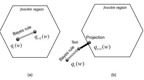
Figure 1: Graphical Illustration of BayesPA learning. (a). Update passivelyby Bayes rule, if the resulting distribution suffer zero loss. (b)Otherwise, aggressively project the resulting distribution to the feasible region of weights with zero loss.
whereFtcan be some family of distributions or the whole probability simplexP. For notational convenience, we denote the objective asL(q(w)). In words, we find a post-data posterior distribu-tionqt+1(w)in the feasible region that is not only close to the current posteriorqt(w)in terms of KL-divergence, but also has a high likelihood of explaining the new data. As a result, if Bayes’ rule already gives the posterior distributionqt+1(w)∝qt(w)p(xt|w)that suffers no loss (i.e.,` = 0), BayesPApassivelyupdates the posterior following just Bayes’ rule;3 otherwise, BayesPA aggres-sivelyprojects the new posterior to the feasible region of posteriors that attain zero loss. The passive and aggressive update cases are illustrated in Figure 1. We should note that when no likelihood is defined (e.g., p(xt|w) is independent of w), BayesPA will passively set qt+1(w) = qt(w) if
qt(w)suffers no loss; otherwise, it will aggressively projectqt(w)to the feasible region. We call it
non-likelihoodBayesPA.
In practical problems, the constraints in (5) could be unrealizable. To deal with such cases, we introduce the soft-margin version of BayesPA learning, which is equivalent to minimizing the objective functionL(q(w))in problem (5) with a regularization term, similar as in SVMs (Cortes and Vapnik, 1995):
qt+1(w) = argmin q(w)∈Ft
Lq(w)+ 2c·`
q(w);xt, yt
. (6)
For the max-margin classifiers that we consider, two types of loss functionals`(q(w);xt, yt)are common:
Methods Max-margin learning ? Bayesian inference ? Streaming update ?
PA yes no yes
SVB no yes yes
RegBayes yes yes no
BayesPA yes yes yes
Table 1: The comparison between BayesPA and its various precursors, including online PA, stream-ing variational Bayes (SVB) and regularized Bayesian inference (RegBayes), in three dif-ferent aspects.
1. Averaging classifier: assume that a post-data posterior distribution q(w) is given, then an averaging classifier makes predictions using the sign ruleyˆt =signEq(w)[w>xt]when the discriminant function has the simple linear form,f(xt;w) = w>xt. For this classifier, its hinge loss is therefore defined as:
`ave
q(w);xt, yt
=
−ytEq(w)
h
w>xt
i
+.
2. Gibbs classifier: assume that a post-data posterior distributionq(w) is given, then a Gibbs classifier randomly draws a weight vectorw∼q(w)to make predictions using the sign rule
ˆ
yt=signw>xt, when the discriminant function has the same linear form as above. For each singlew, we can measure its hinge loss(−ytw>xt)+. To account for the randomness of w, the expected hinge loss of a Gibbs classifier is therefore defined as:
`gibbs
q(w);xt, yt
=Eq(w)
−ytw>xt
+
.
They are closely connected via the following lemma due to the convexity of the function(x)+.
Lemma 1 The expected hinge loss`gibbs is an upper bound of the hinge loss`ave , that is,
`gibbs
q(w);xt, yt
≥`ave
q(w);xt, yt
.
BayesPA is deeply connected to its various precursors reviewed in Section 3, as summarized in Table 1. First, BayesPA is a natural Bayesian extension of online PA, which is explicated via the following theorem. Note that this theorem only serves as a connection to PA, and will not be relied on by our algorithms, where we are more interested in the cases with nontrivial likelihood models to describe the underlying structures (e.g., topic structures), which are typically out-of-reach for the standard PA. Nevertheless, the idea of the proof details would later be applied to develop practical BayesPA algorithms for topic models. Therefore, we include the complete proof here.
Theorem 2 If the prior is normalq0(w) =N(w0, I),Ft=P, and we use the averaging classifier
Proof The soft-margin version of BayesPA learning can be reformulated using a slack variableξt:
qt+1(w) = argmin
q(w)∈P
KLhq(w)||qt(w)
i
+ 2c·ξt
s.t.:ytEq(w)
w>xt
≥−ξt, ξt≥0.
(7)
Similar to Corollary 5 in (Zhu et al., 2012), the optimal solutionq∗(w)of the above problem can be derived from its functional Lagrangian and has the following form:
q∗(w) = 1
Γ(τt∗,xt, yt)
qt(w) exp
τt∗ytw>xt
, (8)
where the normalization termΓ(τt,xt, yt) =
R
wqt(w) exp
τtytw>xt
dw, andτt∗is the optimal solution to the dual problem
max
τt
τt−log Γ(τt,xt, yt)
s.t. 0≤τt≤2c.
(9)
Using this primal-dual interpretation, we prove that for the normal priorp0(w) = N(w0, I), the post-data posterior is also Gaussian: qt(w) = N(µt, I) for someµtin each roundt = 0,1,2, ... This can be shown by induction. By our assumption,q0(w) = p0(w) = N(w0, I) is Gaussian. Assume for roundt≥0, the distributionqt(w) =N(µt, I). Then for roundt+ 1, Eq. (8) suggests the distribution
qt+1(w) =
C
Γ(τt∗,xt, yt)
exp
−1
2||w−(µt+τ
∗
tytxt)||2
,
where the constant C = exp(ytτt∗µ>t xt + 12τt∗2x>txt) . Therefore, the distribution qt+1(w) =
N(µt+τt∗ytxt, I), and the normalization term isΓ(τt,xt, yt) = (
√
2π)Kexp(τtytx>tµt+12τt2x>txt) for anyτt∈[0,2c].
Next, we show thatµt+1 = µt+τt∗ytxtis the optimal solution of the online PA update rule (Crammer et al., 2006). To see this, we replaceΓ(τt,xt, yt)in problem (9) with our derived form. Ignoring constant terms, we obtain the dual problem
max
τt
τt−12τt2x>t xt−ytτtµ>t xt s.t.: 0≤τt≤2c,
(10)
which is exactly the dual form of the online PA update equation:
µPAt+1= arg min µ
1
2||µ−µt||
2+ 2c·ξ t
s.t. ytµ>xt≥−ξt, ξt≥0.
The optimal solution isµPA
t+1 =µt+τt∗ytxt. Note thatτt∗ is the optimal solution of dual problem (10) shared by both PA and BayesPA. Therefore, we conclude thatµt+1 =µPAt+1.
Lemma 3 IfFt =P and we use the averaging classifier with loss functional`ave
, the update rule
of online BayesPA is
qt+1(w) =
1 Γ(τt∗,xt, yt)
qt(w)p(xt|w) exp
τt∗ytw>xt
, (11)
whereΓ(τt,xt, yt)is the normalization termΓ(τt,xt, yt) =
R
wqt(w)p(xt|w) exp
τtytwt>xt
dw,
andτt∗is the optimal solution to the dual problem
max
τt
τt−log Γ(τt,xt, yt)
s.t. 0≤τt≤2c.
For Gibbs classifiers, we have the following lemma to characterize its streaming update rule.
Lemma 4 IfFt =P and we use the Gibbs classifier with loss functional`gibbs , the update rule of
online BayesPA is
qt+1(w) =
qt(w)p(xt|w) exp
−2c −ytw>xt
+
Γ(xt, yt)
, (12)
whereΓ(xt, yt)is the normalization constant.
In both update rules (11) and (12), the post-data posterior qt(w) in the previous round t can be treated as a prior, while the newly observed data and the loss it incurs provide a likelihood and an un-normalized pseudo-likelihood respectively. Due to the analytical form, the BayesPA update rule (12) is sequential in nature, simiar as the convential Bayes rule (3). Therefore, the sequential posterior at timeT is the same as the batch posterior that observes all the data instances up toT. For the case with averaging classifers, Eq. (11) reduces to the streaming Bayesian update problem if there is no loss functional (i.e.,` = 0). Therefore, BayesPA is an extension to streaming variational Bayes (SVB) with imposed max-margin posterior constraints.
Finally, the update formulation (6) is essentially a RegBayes problem with a single data point
(xt, yt). Although RegBayes inference is normally intractable, we would show later in the paper how to use variational approximation to bypass the difficulty for specific settings. This would lead to variational approximation algorithmAfor the streaming update of post-data posterior.
Besides treating a single data point at a time, a useful technique in practice to reduce the noise in data is to use mini-batches. Suppose that we have a mini-batch of data points at timetwith an index setBt. LetXt = {xd}d∈Bt,Yt = {yd}d∈Bt. The online BayesPA update equation for this mini-batch can be defined in a natural way:
min
q∈Ft
KLhq(w)||qt(w)
i
−Eq(w)hlogp(Xt|w)
i
+ 2c·`
q(w);Xt,Yt
,
global&variables
local&variables
sampling analysis model&update
draw&a&mini5
batch infer&the&hidden&structure update&distribu8on&of&global&variables
(a) (b)
Ht
Xt,Yt
t=1,2,...,∞ (Xt,Yt) q*
(Ht) q
*
(w,M)
w
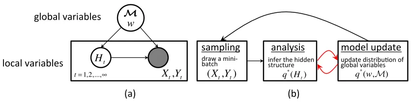
Figure 2: Graphical illustrations of: (a) the abstraction of models with latent structures; and (b) the procedure of BayesPA learning with latent structures.
4.2 BayesPA Learning with Latent Structures
To expressively explain complex real-word data, Bayesian models with latent structures have been extensively developed. The latent structures could typically be characterized by a hierarchy of vari-ables, which are generally grouped into two sets—local latent variableshd(d≥0) that characterize the hidden structures of each observed dataxdandglobal variablesMthat capture the common properties shared by all data.
As illustrated in Figure 2, BayesPA learning with latent structures aims to update the distribution ofMas well as the classifier weights w, based on each incoming mini-batch(Xt,Yt)and their corresponding latent variables Ht = {hd}d∈Bt. Because of the uncertainty in Ht, our posterior approximation algorithmAwould first infer the joint posterior distributionqt+1(w,M,Ht)from
min
q∈Ft
Lq(w,M,Ht)
+ 2c·`
q(w,M,Ht);Xt,Yt
, (13)
where L(q) = KL[q(w,M,Ht)||qt(w,M)p0(Ht)]−Eq(w,M,Ht)[logp(Xt|w,M,Ht)] and
`(q(w,M,Ht);Xt,Yt) is some cumulative loss functional on the min-batch data incurred by some classifiers on the latent variablesHtand/or global variablesM. As in the case without latent variables, both averaging classifier and Gibbs classifier can be used.
Next, algorithmAproduces the approximate posteriorqt+1(w,M). In general we would not obtain a closed-form posterior distribution by marginalizing out Ht, especially in dealing with some involved models like MedLDA (Zhu et al., 2012). The intractability is bypassed through the mean-field assumption q(w,M,Ht) = q(w)q(M)q(Ht). Specifically, algorithmAsolves problem (13) using an iterative procedure and obtain the optimal distributionq∗(w)q∗(M)q∗(Ht). Then it setsqt+1(w,M) =q∗(w)q∗(M)and proceeds to next round. Concrete examples of this method will be discussed in Section 5 and Section 6.
5. Online Max-Margin Topic Models
5.1 Basics of MedLDA
A max-margin topic model consists of a latent Dirichlet allocation (LDA) model (Blei et al., 2003) for describing the underlying topic representations of document content and a max-margin classifier for making predictions. Specifically, LDA is a hierarchical Bayesian model that treats each docu-ment as an admixture ofKtopics,Φ={φk}Kk=1, where each topicφkis a multinomial distribution over a givenW-word vocabulary.4 The generative process of thed-th document (1 ≤ d ≤ D) is described as follows:
• Draw a topic mixture proportion vectorθd|α∼Dir(α)
• For thei-th word in documentd, wherei= 1,2, ..., nd,
– draw a latent topic assignmentzdi ∼Mult(θd).
– draw the word instancexdi∼Mult(φzdi).
where Dir(·)is the Dirichlet distribution and Mult(·)is the multinomial distribution. For Bayesian LDA, the topics are also drawn from a Dirichlet distribution, i.e.,φk ∼Dir(γ).
Given a document set X = {xd}Dd=1. LetZ = {zd}Dd=1 andΘ = {θd}Dd=1 denote all the topic assignments and topic mixing vectors. LDA infers the posterior distributionp(Φ,Θ,Z|X)∝
p0(Φ,Θ,Z)p(X|Z,Φ)via Bayes’ rule. From a variational point of view, the posterior is identical to the solution of the optimization problem:
min
q∈P KL
h
q(Φ,Θ,Z)||p(Φ,Θ,Z|X)i.
The advantage of the variational formulation of Bayesian inference lies in the convenience of posing restrictions on the post-data distribution with a regularization term. For supervised topic models (Blei and McAuliffe, 2010; Zhu et al., 2012), such a regularization term could be a loss function of a prediction model w on the data X = {xd}d=1D and response signalsY = {yd}Dd=1. As a regularized Bayesian (RegBayes) model, MedLDA infers a distribution of the latent variablesZas well as classification weightswby solving the problem:
min
q∈P L
q(w,Φ,Θ,Z)
+ 2c
D
X
d=1
`
q(w,zd);xd, yd
,
where L(q(w,Φ,Θ,Z)) = KL[q(w,Φ,Θ,Z)||p(w,Φ,Θ,Z|X)]. To specify the loss function, a linear discriminant function needs to be defined with respect towandzd
f(w,zd) =w>z¯d, (14)
wherez¯dk = n1d
P
iI[zdi =k]is the average frequency of assigning the words in documentdto topick. Based on the discriminant function, both averaging classifiers with the hinge loss
`ave (q(w,zd);xd, yd) = −ydEq(w,zd)[f(w,zd)]
+, (15) 4. Without causing confusion, we slightly abused the notationKto denote the topic number (i.e., the latent dimension)
and Gibbs classifiers with the expected hinge loss
`gibbs (q(w,zd);xd, yd) =Eq(w,zd)
(−ydf(w,zd))+
, (16)
have been proposed, with extensive comparisons reported in Zhu et al. (2014b) using batch learning algorithms. As commented in (Chang and Blei, 2010), defining the classifier on z¯d, instead of θd, enforces words and labels to share the same topics. Besides, it retains the conjugacy structure between the Dirichlet prior ofθand the multinomial likelihood of generatingz; and it will allow us to integrate outθfor efficient collapsed inference.
5.2 Online MedLDA
We first apply online BayesPA to MedLDA with averaging classifiers, which will be referred to as paMedLDAavefor convenience. During inference, we integrate out the local variablesΘtusing the conjugacy between a Dirichlet prior and a multinomial likelihood (Griffiths and Steyvers, 2004; Teh et al., 2006b), which potentially improves the inference accuracy. Then we have the global variables
M=Φand local variablesHt=Zt. The latent BayesPA rule (13) becomes:
min
q,ξd KL
h
q(w,Φ,Zt)||qt(w,Φ)p0(Zt)p(Xt|Φ,Zt)
i
+ 2c X
d∈Bt
ξd, (17)
s.t.: ydEq(w,zd)[w >
¯
zd]≥−ξd, ξd≥0, ∀d∈Bt,
q(w,Φ,Zt)∈ P.
Since directly solving the above problem is intractable, we would impose a mild mean-field assump-tionq(w,Φ,Zt) =q(w)q(Φ)q(Zt). Now, problem (17) can be solved using an iterative procedure that alternately updates each factor distribution (Jordan et al., 1998), as detailed below:
1. Update globalq(Φ): By fixing the distributionsq(Zt)andq(w), we can ignore irrelevant terms and solve
min
q(Φ) KL
h
q(Φ)q(Zt)||qt(Φ)p0(Zt)p(Xt|Φ,Zt)
i .
The optimal solution has the following closed form:
q∗(Φk)∝qt(Φk) exp
Eq(Zt)
h
logp0(Zt)p(Xt|Zt,Φ)
i
, k= 1,2, ..., K. (18)
If initially the prior is q0(Φk) = Dir(∆0k1, ...,∆0kW), then by induction the inferred distri-butions in each round are also in the family of Dirichlet distridistri-butions, namely, qt(Φk) = Dir(∆tk1, ...,∆tkW). Using equation (18), we can derive
q∗(Φk) =Dir(∆∗k1, ...,∆∗kW), (19)
where∆∗kw = ∆tkw+P
d∈Bt
Pnd
i=1γdik ·I[xdi =w]for all wordsw(1 ≤ w ≤ W) in the vocuabulary andγdik =Eq(zd)I[zdi=k]is the probability of assigning each wordxdito topic
2. Update global weightq(w): Keeping all the other distributions fixed,q(w)can be solved as
min
q(w) KL
h
q(w)||qt(w)
i
+ 2cX
d∈Bt
ξd,
s.t.: ydEq(w)[w]>zbd≥−ξd, ξd≥0, ∀d∈Bt,
wherezbd = Eq(zd)[z¯d]is the expectation of topic assignments under the fixed distribution
q(Z). Similar to Proposition 2 in MedLDA (Zhu et al., 2012), the optimal solution is attained by solving the Lagrangian form with respect toq(w), which gives
q∗(w) = 1
Z(τd∗)qt(w) exp
X
d∈Bt
τd∗ydw>zbd
, (20)
where the Lagrange multipliersτd∗(d∈Bt)are obtained by solving the dual problem
max
0≤τd≤2c
X
d∈Bt
τd−logZ(τd).
For the common spherical Gaussian priorq0(w) = N(0, σ2I), by induction the distribution
qt(w) =N(µt, σ2I)at each round. So equation (20) givesq∗(w) =N(µ∗, σ2I), where
µ∗ =µt+σ2
X
d∈Bt
τd∗ydzbd. (21)
Furthermore, the dual problem becomes,
max
0≤τd≤2c
X
d∈Bt
τd−
X
d1,d2∈Bt
1 2σ
2τ d1τd2zb
>
d1zbd2−µ
> t
X
d∈Bt
ydτdzbd, (22)
which is identical to the Lagrangian dual of the classical PA problem with mini-batch Bt (expressed in the equivalent constrained form by introducing slack variables)
min
µ
||µ−µt||2
2σ2 + 2c
X
d∈Bt
−ydµ>zbd
+. (23)
This equivalence suggests that we could rely on contemporary PA techniques to solve forµ∗. In particular, for instances coming one at a time (i.e.,Bt={t}, ∀t), we have the closed-form solution
τt∗ = min (
2c, −ytµ
> t zbt
+
||zbt||2
)
,
Aitbe the set of instances inBtthat suffer non-zero loss at stepi, then we use the gradients to iteratively update
µi+1 ←µi−ρi∇i, (24)
where annealing rateρi=σ2i−1and
∇i =
µi−µt
σ2 −2c
X
d∈Ai t
ydzbd.
Correspondingly, we can derive the gradient-based update rule for the dual parameters. Imag-ine that we implicitly maintain the relationshipµ= µt+σ2Pd∈Btτdydzbd. Then the
fol-lowing update rule forτd(d∈Bt)naturally implies the update rule (24) forµ:
τdi ←
(1− 1i)τi d+
2c
i ford∈Ait
(1− 1i)τdi ford6∈Ait.
Therefore, the gradient steps adaptively adjust the contribution of each latentzbdtoµbased on
the loss it incurs. Furthermore, the annealing makes sure that0≤τdi ≤2cfor alli. Since the problem (22) is concave, it can be guaranteed thatτdi converges toτd∗. This correspondence would be used in updatingq(Zt).
3. Update localq(Zt): Fixing all the other distributions, we aim to solve
min
q(Zt) KL
h
q(Zt)||p0(Zt)p(Xt|Zt,Φ)
i
+ 2c X
d∈Bt
ξd,
s.t.: ydµ∗>Eq(zd)[z¯d]≥−ξd, ξd≥0, ∀d∈Bt,
whereµ∗ =Eq(w)[w]is the expectation ofwunder the fixed distributionq(w). Unlike the weightw, the expectation overZtduring optimization is intractable due to the combinatorial space of values. Instead, we adopt the same approximation strategy as MedLDA (Zhu et al., 2012): fixξ, τdat the previous global step, and use the approximate solution
q∗(Zt) =p0(Zt)p(Xt|Zt,Φ) exp
X
d∈Bt
τd∗ydµ∗>z¯d
.
Then the expectation ofz¯d, as needed in the global updates, could be approximated by sam-ples from the distributionq∗(Zt). Specifically, we use Gibbs sampling with the conditional distribution
q(zdi=k|Zt¬di)∝ α+Cdk¬di
exp Λk,xdi+
P
d∈Bt
n−1d ydτd∗µ∗k
!
. (25)
whereΛzdi,xdi =Eq(Φ)[log(Φzdi,xdi)] = Ψ(∆ ∗
zdi,xdi)−Ψ(
P
w∆∗zdi,w)(note thatΨ(·)is the digamma function) and Cd¬di is a vector with thek-th entry being the number of words in documentd(except thei-th word) that are assigned to topick.
Then we drawJ samples{Zt(j)}j=1J using Eq. (25), discard the firstβ(0≤β <J) burn-in samples, and approximatezbdkwith the empirical sum(J −β)−1
PJ
j=β+1
P
Algorithm 1Online MedLDA
1: Letq0(w) =N(0;σ2I), q0(φk) =Dir(γ), ∀k. 2: fort= 0→ ∞do
3: Setq(Φ,w) =qt(Φ)qt(w). InitializeZt. 4: fori= 1→ Ido
5: Draw samples{Zt(j)}Jj=1from Eq. (25). 6: Discard the firstβburn-in samples (β <J).
7: Use the restJ −βsamples to updateq(Φ,w)following Eq.s (19, 20). 8: end for
9: Setqt+1(Φ,w) =q(Φ,w). 10: end for
At each roundtof BayesPA optimization during training, we run the global and local updates alternately until convergence, and assignqt(Φ,w) = q∗(Φ)q∗(w), as outlined in Algorithm 1. To make predictions on testing data, we use the mean µas the classification weight and apply the prediction rule. The inference ofz¯for testing documents is similar to Zhu et al. (2014b). First, we draw a single sample ofΦ, and for each test documentd, we infer the MAP ofθd. Then, we directly run the sampling ofzduntil the burn-in stage is completed, and use the average of several samples to computezbd. Then the prediction rule is applied onµandzbd.
5.3 Online Gibbs MedLDA
In this section, we apply the theory of BayesPA to Gibbs MedLDA. As shown in Zhu et al. (2014b), using Gibbs classifiers admits efficient inference algorithms by exploringdata augmentation(DA) techniques (Tanner and Wong, 1987; Polson and Scott, 2011). Based on this insight, we will develop our efficient online inference algorithms for Gibbs MedLDA. We denote the model by paMedLDAgibbs . Specifically, letζd=−ydf(w,zd)andψ(yd|zd,w) = e−2c(ζd)+. By Lemma 4, the optimal solution to problem (13) is
qt+1(w,M,Ht) =
qt(w,M)p0(Ht)p(Xt|Ht,M)ψ(Yt|Ht,w)
Γ(Xt,Yt)
,
where ψ(Yt|Ht,w) = Qd∈Btψ(yd|hd,w) andΓ(Xt,Yt) is a normalization constant. The ba-sic idea of DA is to construct conjugacy between prior and data during inference by introducing augmented variables. Specifically, we would use the following equality (Zhu et al., 2014b):
ψ(yd|zd,w) =
Z ∞
0
ψ(yd, λd|zd,w)dλd, (26)
whereψ(yd, λd|zd,w) = (2πλd)−1/2exp
−(λd+cζd)2 2λd
. Equality (26) essentially implies that the collapsed posteriorqt+1(w,Φ,Zt)is a marginal distribution of
qt+1(w,Φ,Zt,λt) =
p0(Zt)qt(w,Φ)p(Xt|Zt,Φ)ψ(Yt,λt|Zt,w)
Γ(Xt,Yt)
,
whereψ(Yt,λt|Zt,w) =Qd∈Btψ(yd, λd|zd,w)andλt={λd}d∈Bt are augmented variables locally
solution to the problem:
min
q∈P L
q(w,Φ,Zt,λt)
−Eq
h
logψ(Yt,λt|Zt,w)
i
, (27)
whereL(q(w,Φ,Zt,λt)) =KL[q(w,Φ,Zt,λt)kqt(w,Φ)p0(Zt)]−Eq[logp(Xt|Zt,Φ)]. In fact, this objective is an upper bound of that in the original problem (13) (See Appendix A for details).
Again, with the mild mean-field assumption thatq(w,Φ,Zt,λt) = q(w,Φ)q(Zt,λt), we can solve problem (27) via an iterative procedure that alternately updates each factor distribution (Jordan et al., 1998), as detailed below.
1. Global Update: By fixing the distribution of local variables, q(Zt,λt), and ignoring irrele-vant terms, the optimal distribution ofwandΦcan be shown to have the induced factorization form,q(w,Φ) = q(w)q(Φ). Forq(Φ), the update rule is exactly (19). Forq(w), we have the update rule
qt+1(w)∝qt(w) exp
Eq(Zt,λt)
h
logp0(Zt)ψ(Yt,λt|Zt,w)
i .
If the initial prior is normalq0(w) = N(w;µ0,Σ0), by induction we can show that the in-ferred distribution in each round is also a normal distribution, namely,qt(w) =N(w;µt,Σt). Indeed, the optimal solution ofq(w)to problem (27) is
q∗(w) =N(w;µ∗,Σ∗), (28)
where the posterior paramters are computed as
Σ∗=
(Σt)−1+c2
X
d∈Bt
Eq(zd,λd)
h
λ−1d z¯dz¯d>
i
−1
,
µ∗=Σ∗
(Σt)
−1
µt+c X
d∈Bt
Eq(zd,λd)
yd 1 +cλ−1d
¯ zd .
For the sequential update rule, we simply setµt+1=µ∗andΣt+1 =Σ∗.
2. Local Update: Given the distribution of global variables, q(Φ,w), the mean-field update equation for(Zt,λt)is
q(Zt,λt)∝p0(Zt)
Y d∈Bt 1 √ 2πλd exp X
i∈[nd]
Λzdi,xdi−Eq(Φ,w)
(λd+cζd)2
2λd
,
Algorithm 2Online Gibbs MedLDA
1: Letq0(w) =N(0;σ2I), q0(φk) =Dir(γ), ∀k. 2: fort= 0→ ∞do
3: Setq(Φ,w) =qt(Φ)qt(w). InitializeZt. 4: fori= 1→ Ido
5: Draw samples{Zt(j),λ(j)t }Jj=1from Eq.s (29, 30). 6: Discard the firstβburn-in samples (β <J).
7: Use the restJ −βsamples to updateq(Φ,w)following Eq.s (19, 28). 8: end for
9: Setqt+1(Φ,w) =q(Φ,w). 10: end for
• ForZt: By canceling out common factors, the conditional distribution of one variable
zdigivenZt¬diandλtis
q(zdi=k|Zt¬di,λt)∝(α+Cdk¬di)exp
cy
d(c+λd)µ∗k ndλd
+Λk,xdi− c2(µ∗2
k +Σ ∗ kk+2(µ
∗ kµ
∗+Σ∗ ·,k)
>C¬di d ) 2n2
dλd
, (29)
whereΣ∗·,kis thek-th column ofΣ∗.
• Forλt: Letζ¯d = −ydz¯>dµ
∗. The conditional distribution of each variableλ dgiven Ztis
q(λd|Zt)∝
1 √ 2πλd exp −c
2z¯> dΣ
∗z¯
d+ (λd+cζ¯d)2
2λd
=GIG
λd;
1 2,1, c
2ζ¯2
d+ ¯zd>Σ∗z¯d
, (30)
a generalized inverse gaussian distribution (Devroye, 1986). Therefore,λ−1d follows an inverse gaussian distribution, that is,
q(λ−1d |Zt) =IG
λ−1d ;
1
c q
¯
ζd2+ ¯zd>Σ∗z¯d
,1
,
from which we can draw a sample in constant time (Michael et al., 1976).
For training, we run the global and local updates alternately until convergence at each round of PA optimization, as outlined in Alg. 2. To make predictions on testing data, we then draw one sample ofwˆas the classification weight and apply the prediction rule. The inference ofz¯for testing documents is the same as online MedLDA.
6. Extensions
We now present extensions of online MedLDA to automatically determine the unknownK values by leveraging nonparametric Bayesian techniques. We also present an extension of these models for multi-task learning.
6.1 Online Nonparametric MedLDA
We first present online nonparametric MedLDA for resolving the unknown number of topics, based on the theory of hierarchical Dirichlet process (HDP) (Teh et al., 2006a).
6.1.1 BATCHMEDHDP
A two-level HDP provides an extension to LDA that allows for a nonparametric inference of the unknown topic numbers. The generative process of HDP can be summarized using a stick-breaking construction (Wang and Blei, 2012b), where the stick lengthsπ={πk}∞k=1 are generated as:
πk= ¯πk Q i<k
(1−π¯i), π¯k ∼Beta(1, η), fork= 1, ...,∞,
and the topic mixing proportions are generated asθd∼Dir(απ), ford= 1, ..., D. Each topicφk is a sample from a Dirichlet base distribution, i.e., φk ∼ Dir(γ). After we get the topic mixing proportionsθd, the generation of words is the same as in the standard LDA.
To extend the HDP topic model for predictive tasks, we introduce a classifierwthat is drawn from a Gaussian process,GP(0,Σ), where the covariance function isΣ(w,w0) = σ2I[w = w0]. We still define the linear discriminant function in the same form as Eq. (14). Since the number of words in a document is finite, the average topic assignment vectorz¯dhas only a finite number of non-zero elements, and the dot product in Eq. (14) is in fact finite. Therefore, given the latent topic assignments, the conditoinal posterior ofwis in fact a multivariate Gaussian distribution.
Letπ¯ ={¯πk}∞k=1. We define maximum entropy discrimination HDP (MedHDP) topic model as solving the following RegBayes problem to infer the joint post-data posteriorq(w,π¯,Φ,Θ,Z):5
min
q∈PL
q(w,π¯,Φ,Θ,Z)+ 2c
D
X
d=1
`
q(w,zd);xd,yd
, (31)
whereL(q(w,π¯,Φ,Θ,Z)) = KL[q(w,π¯,Φ,Θ,Z)||p(w,π¯,Φ,Θ,Z|X)]is the objective cor-responding to the standard Bayesian inference under the variational formulation of Bayes’ rule. The loss function could be either (15) or (16). We call the resulting model with the averaging classifier MedHDPaveand that with the Gibbs classifier MedHDPgibbs.
Since MedHDP is a new model, we would briefly discuss the corresponding inference problem. For the inference of MedHDPgibbs, we can use Gibbs sampling based on Chinese Restaurant Fran-chise (Teh et al., 2006a; Wang and Blei, 2012a) with modifications similar to the techniques intro-duced in Zhu et al. (2014b). For MedHDPave, the current state-of-the-art for inferring max-margin Bayesian models with averaging loss resorts to mean-field assumptions and variational inference. Notice that classical mean-field derivation would fail due to the potentially unbounded space of variables. However, it is possible to incorporate Gibbs sampling into mean-field update equations to explore the unbounded space (Welling et al., 2008; Wang and Blei, 2012b) and therefore bypass the difficulty. In this paper, we would not focus on developing inference algorithms for MedHDP,
but instead attain batch MedHDP algorithms from the corresponding BayesPA methods, as will be clear at the end of each subsection below.
6.1.2 ONLINEMEDHDP
To apply the ideas of BayesPA to develop online MedHDP algorithms, we have the global variables
M = (π¯,Φ), and the local variablesHt = (Θt,Zt). As in online MedLDA, we marginalize outΘtby conjugacy. Furthermore, to simplify the sampling scheme, we introduce another set of auxiliary latent variablesSt = {sd}d∈Bt, where sd ={sdk}
∞
k=1 and each elementsdk represents the number of occupied tables serving dish k in a Chinese restaurant process (CRP) (Teh et al., 2006a; Wang and Blei, 2012b). By definition, we havep(Zt,St|π¯) =Qd∈Btp(sd,zd|π¯)and
p(sd,zd|π¯)∝ ∞
Y
k=1
S(ndz¯dk, sdk)(απk)sdk, (32)
where S(a, b) are unsigned Stirling numbers of the first kind (Antoniak, 1974). It is not hard to verify that p(zd|π¯) = Psdp(sd,zd|π¯). After this “collapse-and-augment” procedure, we now have the local variables Ht = (Zt,St). The global variables remain intact. The new BayesPA problem is now:
min
q∈Ft
Lq(w,π¯,Φ,Ht)
+ 2c X
d∈Bt
`
w;xt, yt
, (33)
where L(q(w,π¯,Φ,Ht)) = KL[q(w,π¯,Φ,Ht)||qt(w,π¯,Φ)p(Zt,St|π¯)p(Xt|Zt,Φ)] . As in online MedLDA, we adopt the mild mean field assumptionq(w,π¯,Φ,Ht) =q(w)q(π¯)q(Φ)q(Ht) and solve problem (33) via an iterative procedure detailed below.
1. Global Update: By fixing the distribution of local variables,q(Ht), and ignoring the irrel-evant terms, we have same mean-field update equations (19) forΦand (21) forwwith the averaging loss. For global variableπ¯, we have
q∗(¯πk)∝qt(¯πk)
Y
d∈Bt
exp
Eq(hd)
h
logp(sd,zd|π¯)
i
. (34)
By induction, we can show thatqt(¯πk) =Beta(utk, vkt)is a Beta distribution at each step, and the update equation is
q∗(¯πk) =Beta(u∗k, v ∗
k), (35)
where u∗k = utk +P
d∈BtEq(sd)[sdk] and v ∗
k = vkt +
P
d∈BtEq(sd)[
P
j>ksdj] for k =
{1,2, ...}andu0k= 1, v0k=η.
SinceZt contains only a finite number of discrete variables, we only need to maintain and update the above global distributions for a finite number of topics.
2. Local Update:Fixing the global distributionq(w,π¯,Φ), we get the mean-field update equa-tion for(Zt,St):
where
˜
q(Zt,St) = exp Eq∗(Φ)q∗(¯π)[logp(X|Φ,Zt) + logp(Zt,St|π¯)],
ˆ
q(Zt) = exp
X
d∈Bt
τdydE[w]>z¯d
,
andτd(d∈Bt)are the dual variables computed in the global update. The most cumbersome point to tackle is the potentially unbounded sample space ofZt andSt. We take the ideas from (Wang and Blei, 2012b) and adopt an approximation forq(˜Zt,St):
˜
q(Zt,St)≈Eq∗(Φ)q∗(¯π)[p(X|Φ,Zt)p(Zt,St|π¯)]. (37)
Computing the expectation regardingπ¯ in (37) turns out to be difficult. However, imagine that the expectation operator is essentially collapsingπ¯ out from the joint distribution
˜
q(π¯,Zt,St)≈Eq∗(Φ))[q∗(π¯)p(X|Φ,Zt)p(Zt,St|π¯)]. (38)
Now we propose to uncollapseπ¯and sample the local variables from
q∗(π¯,Zt,St)∝q(˜π¯,Zt,St)ˆq(Zt). (39)
Notice in the local updates,π¯ is only an auxilary variable. Putting all the pieces together, we have the following sampling scheme.
• ForZt: LetK be the current inferred number of topics. The conditional distribution of one variable zdi given all other local variables can be derived from (36) with sd marginalized out for convenience.
q(zdi=k|Zt¬di,π¯)∝
(απk+Cdk¬di)(Ckx¬didi+ ∆tkxdi)
P
w(Ckw¬di+ ∆tkw)
exp
X
d∈Bt
n−1d ydτdµ∗k
.(40)
Besides, for k > K and symmetric Dirichlet prior γ, (40) converge to a single rule
q(zdi = k|Zt¬di,π¯) ∝ απk/W, and therefore the total probability of assigning a new topic is
q(zdi> K|Zt¬di,π¯)∝α 1− K
X
k=1
πk
!
/W.
• ForSt: The conditional distribution ofsdk given(Zt,π¯,λt)can be derived from the joint distribution (32):
q(sdk|Zt,π¯)∝S(ndz¯dk, sdk)(απk)sdk. (41)
• Forπ¯: It can be derived from (36) that given(Zt,St), eachπ¯kfollows the beta distri-bution,
¯
πk∼Beta(ak, bk), (42)
whereak=u∗k+
P
d∈Btsdk andbk=v ∗ k+
P
d∈Bt
P
Similar to online MedLDA, we iterate the above steps till convergence for training. For testing, the learned model is essentially a finite MedLDA, and we use the same scheme as that of online MedLDA.
Notice that if we run online MedHDP for only one round (T = 1) and use the entire dataset as mini-batch (|B|= D), iterating the above steps till converge in fact solves the batch MedHDP problem Eq. (31). We call this batch version MedHDPave, and will use it as a baseline algorithm. 6.1.3 ONLINEGIBBSMEDHDP
For Gibbs MedHDP, the only difference is the loss functional`, which is reflected in the sampling of local variables. As in online Gibbs MedLDA, we can facilitate more efficient inference by adopting the same data augmentation technique with the augmented variablesλt. Then the local variables are (Zt,St,λt) and the global variables are unchanged. We then use the mean field assumption
q(w,π¯,Φ,Ht) =q(w)q(π¯)q(Φ)q(Ht)and compute the iterative steps as follows.
1. Global Update: The same as online MedHDP, except that the update rule forwis now (28) for the Gibbs classifier.
2. Local Update: This step involves drawing samples of the local variables. We develop a Gibbs sampler, which iteratively drawsSt from the local conditional in (41), drawsπ¯ from the conditional in (42), and draws the augmented variablesλtfrom the conditional in (30). ForZt, we explain the sampling procedure in detail. Specifically, we inferZtthrough
q∗(Zt,St,λt,π¯)∝q(˜π¯,Zt,St)ˆq(Zt,λt), (43)
where
ˆ
q(Zt,λt) =
Y
d∈Bt
1
√
2πλd
exp
X
i∈[nd]
Λzdi,xdi−Eq(Φ,w)
(λd+cζd)2
2λd
,
The Gibbs sampling for each variablezdiis
q(zdi=k|Zt¬di,λt,π¯)∝
(απk+Cdk¬di)(C ¬di kxdi+ ∆
t kxdi)
P
w(Ckw¬di+ ∆tkw)
exp cyd(c+λd)µ
∗ k
ndλd
−c
2(µ∗2 k + Σ
∗
kk+ 2(µ
∗ kµ
∗+Σ∗
·,k)>Cd¬di)
2n2dλd
!
, (44)
while the probability of sampling a new topic is
q(zdi> K|Zt¬di,π¯)∝α 1− K
X
k=1
πk
!
/W.
6.2 Multi-task Learning
The above models have been presented for classification. The basic ideas can be applied to solve other learning tasks, such as regression and multi-task learning (MTL). We use multi-task learn-ing an one example. The primary assumption of multi-task learnlearn-ing is that by sharlearn-ing statistical strength in a joint learning procedure, multiple related tasks can be mutually enhanced or some main tasks can be improved. MTL has many applications. We consider one scenario for multi-label classification. In this task, a set of binary classifiers are trained, each of which identifies whether a documentxdbelongs to a specific categoryydq∈ {+1,−1}. These binary classifiers are allowed to share common latent representations and therefore could be attained via a modified BayesPA update equation:
min
q∈Ft
Lq(w,M,Ht)
+ 2c
Q
X
q=1
`
q(w,M,Ht);Xt,Ytτ
,
where Q is the total number of tasks. We can then derive the multi-task version of Passive-Aggressive topic models, denoted by paMedLDAmtave and paMedLDAmtgibbs , in a way similar as in Section 5. We can further develop the nonparametric multi-task MedLDA topic models in a way similar as in Section 6.1 and the online PA learning algorithms. We denote the nonparamet-ric online models by paMedHDPave and paMedHDPgibbs , according to whether the task-specific classifier is averaging or Gibbs.
7. Experiments
We demonstrate the efficiency and prediction accuracy of online MedLDA, online Gibbs MedLDA and their extensions on the 20Newsgroup (20NG) and a large Wikipedia dataset. A sensitivity analysis of the key parameters is also provided. Following the same setting in Zhu et al. (2012), we remove a standard list of stop words. All of the experiments are done on a normal computer with single-core clock rate up to 2.4 GHz.
7.1 Classification on 20Newsgroup
We perform multi-class classification on the entire 20NG dataset with all the 20 categories. The training set contains 11,269 documents, with the smallest category having 376 documents and the biggest category having 599 documents. The testing set contains 7,505 documents, with the smallest and biggest categories having 259 and 399 documents respectively. We adopt the “one-vs-all” strategy (Rifkin and Klautau, 2004) to combine binary classifiers for multi-class prediction tasks.
10−1 100 101 0.2
0.4 0.6 0.8 1
#Passes Through the Dataset
Error Rate
paMedLDAave paMedLDAgibbs MedLDAgibbs gMedLDA spLDA+SVM
10−1 100 101
0.2 0.4 0.6 0.8 1
#Passes Through the Dataset
Error
paMedHDPave paMedHDPgibbs MedHDPave MedHDPgibbs tfHDP+SVM
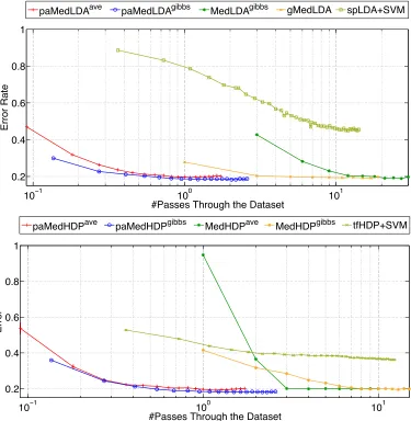
Figure 3: Test errors of different models with respect to the number of passes through the 20NG training dataset.
(Blei and McAuliffe, 2010) and DiscLDA (Lacoste-Julien et al., 2008), as well as SVM classi-fiers on the raw inputs, which are generally either inferior in accuracy or slower in efficiency than MedLDA. For all the LDA-based topic models, we use symmetric Dirichlet priorsα= 1/K·1and
γ = 0.45·1. For BayesPA with Gibbs classifiers, the parameters were set at= 164,c= 1, and
σ2 = 1. The models’ performance is not sensitive to the choice of these parameters in wide ranges as shown in Zhu et al. (2014b). For BayesPA with averaging classifiers, the parameters determined by cross validation are= 16,c= 500, andσ2 = 10−3. For reasons explained in section 7.3, we set the mini-batch size|B|= 1for the averaging classifier and|B|= 512for the Gibbs classifier.
(I,J, β) = (1,2,0). As we can observe, by solving a series of latent BayesPA problems, both paMedLDAaveand paMedLDAgibbsfully explore the redundancy of documents and converge in less than one pass, while their corresponding batch algorithms (i.e., MedLDA and MedLDAgibbs) need many passes as burn-in steps. Besides, compared with the online learning algorithms for unsuper-vised topic models (i.e., spLDA+SVM), BayesPA topic models use supervising side information from each mini-batch, and therefore exhibit a faster convergence rate in discrimination ability. The convergence performance of BayesPA models is significantly better than that of the unsupervised spLDA.
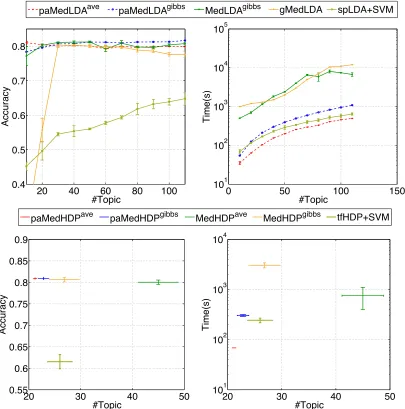
Next, we study each model’s best performance possible and the corresponding training time. To allow for a fair comparison, we train each model until the relative change of its objective is less than10−4. Figure 4 shows the prediction accuracy and training time of LDA-based models on the whole dataset with varying numbers of topics. We can see that BayesPA topic models are more than an order of magnitude faster than their corresponding batch algorithms in training time due to the power of online learning. paMedLDAave is faster than paMedLDAgibbs , because it does not need to update the covariance matrix of classifier weightsw. But the tradeoff is that for averaging models, they are more sensitive to the initial choice of σ2, and therefore we need to use cross-validation to determine the best choice of variance beforehand. Furthermore, thanks to the merits of structured mean-field inference, which does not impose strict assumptions on the independence of latent variables, BayesPA topic models parallel their batch alternatives in accuracy. Moreover, all the supervised models are significantly better than the unsupervised spLDA in classification, reaching the state-of-the-art performance on the tested datasets.
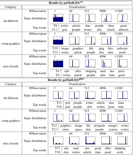
Table 2 visualizes the learnt topic representation by paMedLDAaveand paMedLDAgibbs. For the displayed categories, we plot the corresponding classifier’s topic distribution averaged over the pos-itive examples and top words from the topic matrix. As we can see, the average topic distributions become increasingly sparse as more and more data are observed. Eventually, the averaged topic dis-tribution for each category contains only 1∼2 non-zero entries and meanwhile different categories have quite diverse average topic distributions, therefore showing strong discriminative ability of the topic representations in distinguishing different categories. Such sparse and discriminatrive patterns are similar to what have been shown in batch settings (Zhu et al., 2012, 2014b).
7.2 Extensions
We now present the experimental results on the extensions of BayesPA topic models. We first present the results of nonparametric topic modeling on the same 20NG dataset. Then we demon-strate multi-task learning on a large Wikipedia dataset with more than 1 million documents and about 1 million unique terms.
7.2.1 NONPARAMETRICTOPIC MODELING
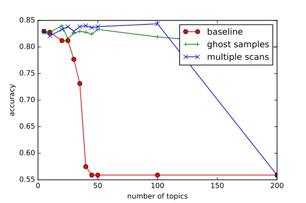
20 40 60 80 100 0.4
0.5 0.6 0.7 0.8
#Topic
Accuracy
paMedLDAave paMedLDAgibbs MedLDAgibbs gMedLDA spLDA+SVM
0 50 100 150
101
102
103
104
105
#Topic
Time(s)
20 30 40 50
0.55 0.6 0.65 0.7 0.75 0.8 0.85 0.9
#Topic
Accuracy
paMedHDPave paMedHDPgibbs MedHDPave MedHDPgibbs tfHDP+SVM
20 30 40 50
101 102 103 104
#Topic
Time(s)
Figure 4: Classification accuracy and running time of various models with respect to the number of topics on the 20NG dataset.
for HDP to start with, we chooseK = 20. We observed that the training time and the prediction accuracy do not depend heavily on the initial number of topics. The other parameters of BayesPA are the same.
Results by paMedLDAave
Category Visualization
alt.altheism
#Observation 1 64 512 4096 11269
Topic distribution
Top words T8 writes article don people time good
T11 god people writes don article atheism
comp.graphics
#Observation 1 64 512 4096 11269
Topic distribution
Top words T19 image graphics file jpeg files software
T13 writes article people don time good
misc.forsale
#Observation 1 64 512 4096 11269
Topic distribution
Top words T4 sale offer shipping mail dos price
T8 writes article people don time good
Results by paMedLDAgibbs
Category Visualization
alt.altheism
#Observation 1 64 512 4096 11269
Topic distribution
Top words T11 god people writes article don time
T16 god people don writes jesus time
comp.graphics
#Observation 1 64 512 4096 11269
Topic distribution
Top words T14 graphics image file program images writes
T13 entry space don people system writes
misc.forsale
#Observation 1 64 512 4096 11269
Topic distribution
Top words T17 sale mail dos good offer shipping
T18 don writes article time good work
100 1 102 103 104 105 0.1
0.2 0.3 0.4 0.5
Time (Seconds)
F1 Score
paMedLDAmtave paMedHDPmtave paMedLDAmtgibbs paMedHDPmtgibbs MedLDAmt MedHDPmt
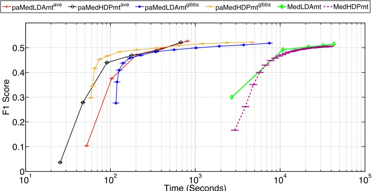
Figure 5: F1 scores of various multi-task topic models with respect to the running time on the 1.1M wikipedia dataset.
7.2.2 MULTI-TASKCLASSIFICATION
We test paMedLDAmtave , paMedLDAmtgibbs and their nonparametric exentions on a large Wiki dataset. The Wiki dataset is built from the Wikipedia set used in PASCAL LSHC challenge 2012 6. The Wiki dataset is a collection of documents with labels up to 20 different kinds, while the data distribution among the labels is balanced. The training set consists of 1.1 millions of wikipedia doc-uments and the testing test consists of 5,000 docdoc-uments. The vocabulary contains 917,683 unique terms. To measure performance, we use F1 score, the harmonic mean of precision and recall.
As baseline batch algorithms, we include MedLDAmt, a recent multi-task extention of Gibbs MedLDA (Zhu et al., 2013). Since MedHDP is a new model, there is no exising implementation of multi-task batch versions. So we instead extended MedHDP to support multi-task inference. We call this model MedHDPmt.
We use the same validation scheme as previous to select batchsize |B| = 1, c = 5000, σ2 = 10−6for paMedLDAmtave; We choose|B|= 512, c= 1, σ2 = 1for paMedLDAmtgibbs. For both models, the Dirichlet parameters areα = 0.8·1,γ = 0.5·1, and = 1. We useK = 40topics for MedLDA models. The nonparametric extensions use exactly the same parameter settings except thatα= 5·1, η = 1and we do not need to specify the topic numberK.
Figure 5 shows the F1 scores of various models as a function of training time. We find that BayesPA topic models produce comparable results with their batch counterparts, but the training time is significantly less. With either Gibbs or averaging classifiers, BayesPA is about two orders of magnitude faster than their batch counterparts. Therefore, BayesPA topic models could potentially be applied to large-scale multi-class settings.
100 101 102 103 104 105 0.2
0.3 0.4 0.5 0.6 0.7 0.8 0.9 1
CPU Seconds (Log Scale)
Test Error
100 101 102 103 104 105
0.2 0.3 0.4 0.5 0.6 0.7 0.8 0.9 1
CPU Seconds (Log Scale)
Test Error
1 4 16 64 256 1024 Batch
Batch Size
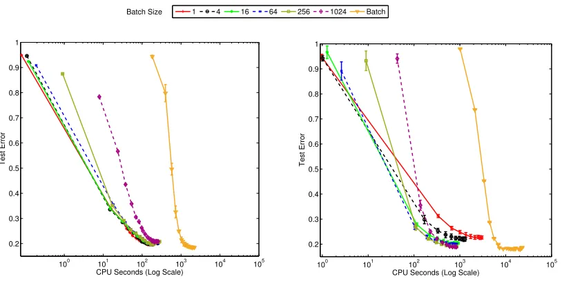
Figure 6: Test errors of paMedLDAave(left) and paMedLDAgibbs (right) with different batch sizes on the 20NG dataset.
7.3 Sensitivity Analysis
We provide further discussions on BayesPA learning for topic models. We analyze the models’ sensitivity to some key parameters.
Batch Size |B|: Figure 6 presents the test errors of BayesPA topic models (paMedLDAave , paMedLDAgibbs) as a function of training time on the entire 20NG dataset with various batch sizes. The number of topics is fixed at K = 40. We can see that the convergence speeds of different algorithms vary. First of all, the batch algorithms suffer from multiple passes through the dataset and therefore are much slower than the online alternatives. Second, we could observe that algo-rithms with medium batch sizes (|B| = 64 or 256) converge faster. If we choose a batch size too small, for example,|B| = 1, each iteration would not provide sufficient evidence for the up-date of global variables; if the batch size is too large, each mini-batch becomes redundant and the convergence rate also decreases. By comparing the two figures, we find that paMedLDAave runs faster than paMedLDAgibbs . This is because for averaging classifers, we do not update the co-varaince of the classifier weights, which requires frequent matrix inverse operations. Furthermore, paMedLDAaveappears to be more robust against change in batchsize. Similarly, Figure 7 shows the sensitivity experiment of the batchsize parameter in paMedHDP models. The results are similar to paMedLDA models, that is, a moderate batchsize leads to faster convergence.