Tests of Mutual or Serial Independence of Random Vectors
with Applications
Martin Bilodeau [email protected]
Aur´elien Guetsop Nangue [email protected]
D´epartement de math´ematiques et de statistique Universit´e de Montr´eal
C.P. 6128, Succursale A Montr´eal, Canada H3C 3J7
Editor:Arthur Gretton
Abstract
The problem of testing mutual independence between many random vectors is addressed. The closely related problem of testing serial independence of a multivariate stationary se-quence is also considered. The M¨obius transformation of characteristic functions is used to characterize independence. A generalization to p vectors of distance covariance and Hilbert-Schmidt independence criterion (HSIC) tests with the translation invariant kernel of a stable probability distribution is proposed. Both test statistics can be expressed in a simple form as a sum over all elements of a componentwise product ofpdoubly-centered matrices. It is shown that an HSIC statistic with sufficiently small scale parameters is equivalent to a distance covariance statistic. Consistency and weak convergence of both types of statistics are established. Approximation of p-values is made by randomization tests without recomputing interpoint distances for each randomized sample. The depen-dogram is adapted to the proposed tests for the graphical identification of sources of de-pendencies. Empirical rejection rates obtained through extensive simulations confirm both the applicability of the testing procedures in small samples and the high level of competi-tiveness in terms of power. Applications to meteorological and financial data provide some interesting interpretations of dependencies revealed by dependograms.
Keywords: Distance covariance, Hilbert-Schmidt independence criterion, M¨obius trans-formation, mutual independence, serial independence
1. Introduction
The problem of testing for independence between p components of a random vector has attracted considerable attention in statistics. Many nonparametric procedures exist in the literature. A natural approach is to consider a functional of the difference between the empirical joint distribution and the product of the empirical marginal distributions. This same approach can also use empirical characteristic functions. When the functional of the difference is above a certain threshold, the components are declared dependent. Cs¨org˝o (1985), Kankainen (1995), Sejdinovic et al. (2013b) and Fan et al. (2017) considered mutual tests of independence based on empirical characteristic functions. However, when dependence is declared, it is not possible to identify, with their proposed tests, subsets of
c
variables responsible for the dependence. This limitation is similar to that of a globalF-test in an analysis of variance model with one fixed factor, as opposed to multiple comparisons procedures, or that of a global chi-square test of independence in a multi-way contingency table, as opposed to log-linear models with interaction terms. For tests of independence, a useful method is the M¨obius transformation.
The M¨obius transformation defined in (1) of Section 2 has a long history in statistics. The M¨obius transformation of distribution functions was first proposed in Blum et al. (1961) forp= 3. The general case was treated in Deheuvels (1981), Ghoudi et al. (2001), Genest and R´emillard (2004), Kojadinovic and Holmes (2009), Kojadinovic and Yan (2011), and Duchesne et al. (2012). It can also be defined with characteristic functions as in Bilodeau and Lafaye de Micheaux (2005), with half-space probabilities as in Beran et al. (2007), or with cell probabilities in a contingency table as in Bilodeau and Lafaye de Micheaux (2009). The first appearance of a M¨obius transformation, although not stated explicitly, goes back to the work of Lancaster (1951) on contingency tables as explained in Bilodeau and Lafaye de Micheaux (2009). The machine learning community (Sejdinovic et al., 2013a) proposed kernel nonparametric tests for Lancaster three-variable interaction. This test is in fact a test based on the empirical version of the M¨obius transformation of the characteristic function when p= 3. The general M¨obius transformation considered in this paper can be used to build tests for general interactions of any order, as well as tests of mutual and serial independence.
The paper is organized as follows. Section 2 introduces the M¨obius transformation of characteristic functions. It presents a characterization of the mutual independence between p random vectors by the M¨obius transformation. In Section 3, new tests based on the M¨obius transformation of empirical characteristic functions are introduced. They general-ize the Hilbert-Schmidt independence criterion (HSIC) test (Gretton et al., 2005, 2008) and the distance covariance test (Sz´ekely et al., 2007) to the case p > 2. This work ad-dresses the case of finite-dimensional Euclidean spaces. HSIC was originally defined more generally using any semimetric space of negative type (as in the distance covariance), or any Borel measurable space on which a kernel is defined (Sejdinovic et al., 2013b). For example, in Gretton et al. (2008), dependence was detected between text in different lan-guages using kernels on strings. On the other hand, this manuscript proposes a criterion that is more general than HSIC in a different respect, via subsets of components in the M¨obius transformation, where the criterion coincides with HSIC when the latter is spe-cialized to Euclidean spaces and p = 2. The new test statistics have a common form as a sum of elements of a componentwise product of p doubly-centered matrices. An equiv-alence is established between an HSIC statistic with infinitesimal scale parameters and a distance covariance statistic. The weak convergence of the empirical processes based on the M¨obius transformation is proved. The consistency and weak convergence of theHSIC and distance covariance functionals are also established. A difficulty encountered in establishing the asymptotic independence of the collection of distance covariance functionals, over all subsets of components, is described. Other competing nonparametric tests of independence are reviewed in Section 4.
the methods of Fisher (1950, pp. 99-101) or Tippett (1952) to obtain a global test of mu-tual independence. Section 7 describes the dependogram, a graphical device of Genest and R´emillard (2004), in the context ofHSIC and distance covariance tests. Section 8 adapts all the results described for the mutual independence situation to the problem of testing for the serial independence of a multivariate stationary sequence. Computational costs are given in Section 9 together with a short description of R(R Core Team, 2015) packages for nonparametric independence tests. Simulated models are considered in Section 10 to verify that the proposed tests have empirical significance levels close to the nominal level in small samples and comparable or higher powers in many situations when compared to existing tests such as those of Cs¨org˝o (1985), Kojadinovic and Holmes (2009) or Kojadinovic and Yan (2011).
Finally, Section 11 contains an application to real data on variables related to air tem-perature, soil temtem-perature, humidity, wind, and evaporation. HSIC or distance covariance tests should be preferred to the Gaussian likelihood ratio test since a multivariate Gaus-sian model is rejected by the test of Henze and Zirkler (1990). According to these tests, wind does not exhibit any dependence with all other variables considered. Another appli-cation finds significant serial dependencies in the S&P/TSX composite, DOW JONES, and S&P500 daily percent increasing rates ranging from January 2, 2014 to March 2, 2016. The strongest dependency observed at a lag of 4 days by a distance covariance test is interpreted using a broken line regression model as the tendency of stock markets to recover in the days following a sharp decline.
2. M¨obius Transformation
The M¨obius transformation of characteristic functions is a powerful tool for the characteri-zation of mutual independence betweenp random vectorsZ(1), . . . , Z(p). The dimension of the vector Z(j) is d
j, for j = 1, . . . , p. Let f be the joint characteristic function of these p
vectors, and let f(j) be the marginal characteristic function of Z(j). Mutual independence is characterized by the factorization
f(t(1), . . . , t(p)) =
p
Y
j=1
f(j)(t(j)),
for all t(1), . . . , t(p). It may also be characterized by the M¨obius transformation which is defined as follows. Let Ip be the family of subsets B of {1, . . . , p} of cardinality |B| >1.
The setIp has 2p−p−1 elements since the empty set is excluded, as well as allpsingletons.
For anyB ∈ Ip and any t(1), . . . , t(p), definet(B) = (t(j) : j∈B). Similarly,Z(B)= (Z(j):
j∈B), andf(B) is the joint characteristic function ofZ(B). The M¨obius transformation of the characteristic function f for the set B ∈ Ip is given by
µB(t(B)) =
X
C⊆B
(−1)|B\C|f(C)(t(C)) Y
j∈B\C
f(j)(t(j)). (1)
By convention, forC=∅, bothf(C)(t(C)) andQ
j∈Cf(j)(t(j)) are equal to one. The following
characterization holds: Z(1), . . . , Z(p)are mutually independent if and only if,µ
for all B ∈ Ip, and all vectors t(B). A proof by induction of this characterization using
distribution functions is given in Ghoudi et al. (2001) and is immediately applicable to characteristic functions.
3. Dependence Statistics
Consider Zk = (Z
(1)
k , . . . , Z
(p)
k ), k = 1, . . . , n, an independent and identically distributed
sample of sizen. The M¨obius processes corresponding toµB,B ∈ Ip, are defined as
RnB(t(B)) =
√ n X
C⊆B
(−1)|B\C|fn(C)(t(C)) Y
j∈B\C
fn(j)(t(j)), (2)
where
f(C)
n (t(C)) =
1 n
n
X
k=1
eiht(C),Zk(C)i (3)
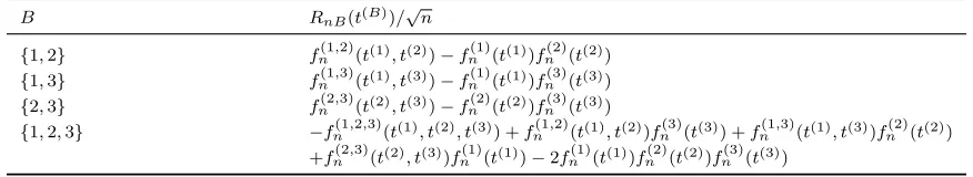
is the empirical characteristic function. WhenC ={j}is a singleton, the notation used for fn(C)is simplyfn(j). The empirical processesRnB, for allB ∈ Ip, are illustrated whenp= 3
in Table 1. The processes RnB are identical to the empirical characteristic independence
processes
SnB(t(B)) =√n
fn(B)(t(B))− Y
j∈B
fn(j)(t(j))
in Cs¨org˝o (1985) only for subsets B of cardinality 2. The process SnB appears later in
the test statistic J2
n in (17) used for testing the hypothesis of mutual independence. For
B ={1,2,3}, the process
SnB(t(B)) =
√
nhfn(1,2,3)(t(1), t(2), t(3))−fn(1)(t(1))fn(2)(t(2))fn(3)(t(3))i
can be contrasted with the processRnB in Table 1. Although, at first sight, RnB may look
more complicated thanSnB and both processes converge weakly to Gaussian processes, the
processes RnB have major advantages which are enunciated in Section 4.
B RnB(t(B))/
√
n
{1,2} fn(1,2)(t(1), t(2))−fn(1)(t(1))fn(2)(t(2))
{1,3} fn(1,3)(t(1), t(3))−f
(1)
n (t(1))f
(3)
n (t(3)) {2,3} fn(2,3)(t(2), t(3))−fn(2)(t(2))fn(3)(t(3))
{1,2,3} −fn(1,2,3)(t(1), t(2), t(3)) +fn(1,2)(t(1), t(2))fn(3)(t(3)) +fn(1,3)(t(1), t(3))fn(2)(t(2))
+fn(2,3)(t(2), t(3))f
(1)
n (t(1))−2f
(1)
n (t(1))f
(2)
n (t(2))f
(3)
n (t(3))
Table 1: Empirical processes RnB,B ∈ I3.
The dependence statistic for the subset B is now defined as the Cram´er-von Mises functional
WnB =
1 n
Z
wheredwB(t(B)) =Qj∈Bdw(j)(t(j)) is a product measure. The evaluation of this integral is
facilitated using another representation of the process. First, recall the multinomial formula (Ghoudi et al., 2001)
X
C⊆B
Y
i∈C
u(i) !
Y
j∈B\C
v(j)
= Y
i∈B
u(i)+v(i). (5)
Then, the empirical process (2) can be written as
RnB(t(B)) =
1 √ n
n
X
k=1 Y
j∈B
h
eiht(j),Zk(j)i−f(j)
n (t(j))
i
. (6)
The representation (6) is obtained after replacing the expression (3) for the empirical char-acteristic function in (2) and by applying the multinomial formula (5). The representation given by (6) allows the integral (4) to be evaluated explicitly in some cases and simplifies the proof of theorems to come. Two important cases are now presented.
3.1 Hilbert-Schmidt Independence Criterion
Assume that the measure dwB(t(B)) =Qj∈BdG(j)(t(j)) is a product of symmetric (around
the origin) probability measures. The population Hilbert-Schmidt independence criterion is
H2
B =
Z
|µB(t(B))|2
Y
j∈B
dG(j)(t(j)) (7)
which is well defined since the function µB is bounded. For the sample version, let ϕ(j)
be the (real) characteristic function of G(j). The sample version of the Hilbert-Schmidt independence criterion (7) is denoted H2
nB and has the following explicit expression.
Theorem 1 For any B ∈ Ip, the dependence statistic HnB2 is given by
H2
nB =
1 n2
n
X
k=1
n
X
l=1 Y
j∈B
A(klj), (8)
where
akl(j) = ϕ(j)(Zk(j)−Zl(j)), (9) Akl(j) = a(klj)−¯ak.(j)−¯a(.lj)+ ¯a(..j),
¯
a(k.j) = 1 n
n
X
l=1
a(klj), ¯a(.lj)= 1 n
n
X
k=1
a(klj), a¯(j)
.. =
1 n2
n
X
k,l=1 a(klj).
By definition, matrices A(j) = (A(j)
kl), j = 1, . . . , p, are doubly-centered, i.e. rows and
columns of these matrices sum up to zero. In the special casep= 2 of testing the indepen-dence between two vectors, the statistic H2
nB, for B ={1,2}, is the Hilbert-Schmidt
inde-pendence criterion, or HSIC, with translation invariant kernels ϕ(j)(Z(j)
k −Z
(j)
l ),j= 1,2.
An important special case is whenG(j) is the stable distribution of indexα∈(0,2] with scale parameterβj >0 first studied by L´evy (1925). Then, the translation invariant kernel
is
a(klj)=e−βjα|Z
(j)
k −Z
(j)
l |αdj, (10)
where| · |dj is the Euclidean norm in dimensiondj. The corresponding dependence statistic
is then denoted HnB2(α). The case α = 2 is the Gaussian kernel, and α = 1 is the Cauchy kernel, often referred to as the Laplace kernel in machine learning (Gretton et al., 2005, 2009) because of its similarity to a Laplace density in dimension one.
The following result establishes the consistency of the Hilbert-Schmidt independence criterion H2
nB.
Theorem 2
(i) H2
nB a.s.
→ H2
B, as n→ ∞.
(ii) If µB(t(B))= 06 for some vector t(B), then nHnB2
a.s.
→ ∞, as n→ ∞.
3.2 Distance Covariance
Assume that the measure dwB(t(B)) = Qj∈Bdw(j)(t(j)) is a product of non integrable
measures. The measuredw(j) of index 0< α <2 is defined as dw(j)(t(j)) =hC(dj, α)|t(j)|ddjj+α
i−1 dt(j), with the normalizing constant
C(d, α) = 2πd/2Γ(1−α/2)/[α2αΓ((d+α)/2)].
A similar representation as in (8) also holds. The corresponding dependence statistic is denoted VnB2(α), which is the usual notation for distance covariance of index α.
Theorem 3 Let 0< α <2. Then, for any B ∈ Ip, the dependence statistic VnB2(α) has the
same form as in (8) of Theorem 1 with
a(klj) =−|Zk(j)−Zl(j)|αdj. (11) In the special case|B|= 2, the statisticVnB2(α) reduces to the distance covariance of indexα
in Feuerverger (1993) for the cased1 =d2 = 1, and later generalized by Sz´ekely et al. (2007) to the cased1 ≥1,d2 ≥1. A very special case requiring a separate analysis is when|B|= 2 and α= 2. In this case,VnB2(2) is the numerator of theRV coefficient of Escoufier (1973) as noticed by Josse and Holmes (2016) when d1 ≥1 and d2 ≥1, and earlier by Sz´ekely et al. (2007) only when d1 =d2 = 1. It should be noted that the case α= 2 leads only to a test of non correlation but not of independence, unless the joint distribution is Gaussian. For this reason, the value α= 2 will not be considered for distance covariance in the sequel.
Theorem 4 Let 0< α <2. Assume
E Y
j∈B
|Z1(j)−Z2(j)|α
dj <∞. (12)
Define
VB2(α) =E
Y
j∈B
h
−|Z1(j)−Z2(j)|αdj +E3|Z1(j)−Z (j) 3 |
α
dj+E3|Z
(j) 2 −Z
(j) 3 |
α
dj−E|Z
(j) 3 −Z
(j) 4 |
α dj
i .
Then,
(i) VB2(α)=R
|µB(t(B))|2dwB(t(B))<∞.
(ii) If µB(t(B))6= 0 for some vector t(B), then nVnB2(α)
a.s.
→ ∞, as n→ ∞.
For 0 < α < 2, the following limit establishes that VnB2(α) is, for all practical purpose, equivalent to H2(nBα) when scale parameters βj,j∈B, are sufficiently small:
lim
βj→0,∀j∈BH
2(α)
nB /
Y
j∈B
βα j =V
2(α)
nB . (13)
This result, proved in the appendix, implies that H2(nBα), properly normalized with suffi-ciently small scale parameters, can be as close as desired to VnB2(α) and thus,H
2(α)
nB will have
a power function indistinguishable from that ofVnB2(α). For semimetrics generated by kernels,
Sejdinovic et al. (2013b, Theorem 24) established an equivalence between distance covari-ance andHSIC. However, for distance covariance defined in terms of a weighted distance between characteristic functions, one can not find a continuous translation invariant kernel for which HSIC coincide with distance covariance (Sejdinovic et al., 2013b, Section 5.3). Nevertheless, (13) provides an equivalence of a different nature: for α-stable distributions, appropriately normalized HSIC and distance covariance are equivalent in the limit, as the scale parameters converge to zero.
As simple as it may seem, this equivalence, for the simplest case |B| = 2, has gone unnoticed in the discussions of distance covariance (Sz´ekely and Rizzo, 2009; Gretton et al., 2009). In Section 8.2 of Sejdinovic et al. (2013b), for |B| = 2, the HSIC test based on H2(2)nB with Gaussian kernels with scale parameters set at the inverse of median of interpoint
distances is compared to distance covariance tests of varying index α. It was found in the independent component analysis benchmark example that VnB2(1/3) is more powerful than
H2(2)nB . From (13), the HSIC test based on H
2(1/3)
nB , with translation invariant kernels of
the stable distribution of index α = 1/3 and very small scale parameters, would have a power function indistinguishable from that ofVnB2(1/3). In another example with sinusoidally
dependent data, theHSIC test based onH2(2)nB has a very poor power function compared to
VnB2(1/6). Sejdinovic et al. (2013b) explained: “the exponent in the distance-induced kernel
lengthscale of the marginal distributions (captured by the median interpoint distances) and the lengthscales at which dependencies are present”. In fact, the exponent in the distance-induced kernel of a distance covariance test plays the same role as the index of the translation invariant kernel of a stable distribution in anHSIC test. Indistinguishable power functions can be obtained by choosing sufficiently small scale parameters in the translation invariant kernel. This all means that HSIC with sufficiently small scale parameters always match distance covariance in terms of power. But HSIC with scale parameters appropriately selected may, in some cases, improve on distance covariance.
3.3 Asymptotic Distribution
Empirical processes as in (2) have been recently very useful at tackling problems related to mutual independence because of the simplicity of the asymptotic distribution. Let dB =
P
j∈Bdj. Each processRnB is defined on the spaceC(RdB,C) of complex-valued continuous functions defined on RdB. Let d=Ppj=1dj and t = (t1, . . . , td) ∈Rd. The following mild tail condition (Cs¨org˝o, 1981, 1985) is assumed
Z 1 0
¯ ψ(h) h log1
h
1/2dh <∞, (14)
where
¯
ψ(h) = sup
y : 0≤y≤1, λd
t: |t|∞<
1
2, ψ(t)< y
< h
,
with λd standing for the Lebesgue measure in Rd and |t|∞ = max(|t1|, . . . ,|td|), is the
nondecreasing rearrangement of the function ψ(t) = [1−Ref(t)]1/2. Weak convergence of the collection of processes RnB is now established. For details concerning the metrics on
the spaces in Theorem 5, the reader is referred to the appendix. The symbol⇒ stands for weak convergence.
Theorem 5 If Z(1), . . . , Z(p) are mutually independent, then the process R
nB ⇒ RB in
C(RdB,C), whereR
B is a zero mean complex Gaussian process withR¯B(t(B)) =RB(−t(B))
and complex covariance function
E h
RB(t(B)) ¯RB(s(B))
i = Y
j∈B
[f(j)(t(j)−s(j))−f(j)(t(j))f(j)(−s(j))].
Moreover, the collection of processes (RnB : B ∈ Ip) ⇒ (RB : B ∈ Ip) on the product
of spaces ×
B∈IpC(R
dB,
C) to a zero mean Gaussian process such that the marginal processes
RB, B ∈ Ip, are mutually independent.
The convergence of functionals (4) also holds even though they are not defined on the whole spaceC(RdB,C), but only on the space of squared integrable functions. In the next
theorem, the asymptotic distribution of nH2
nB is described. In particular, it provides the
asymptotic distribution ofnH2(nBα), for anyα∈(0,2].
Theorem 6 Let WnB = H2nB. If Z(1), . . . , Z(p) are mutually independent, then nWnB ⇒
WB for each B ∈ Ip, where WB =
R
|RB(t(B))|2
Q
of variables (nWnB : B ∈ Ip) ⇒ (WB : B ∈ Ip), where the variables WB, B ∈ Ip, are
mutually independent.
Theorem 6 holds without moment conditions forH2
nB since in this casedwBis a probability
measure. Theorems 5 and 6 were proved when p = 2 by Zhang et al. (2011). The case forp = 3 was covered in Appendix E of Sejdinovic et al. (2013a). The distribution of WB
can be represented using the Karhunen-Lo`eve expansion. Without loss of generality, let B ={1, . . . , k}. Then,WB is distributed as
∞
X
i1=1 · · ·
∞
X
ik=1
λ(1)i1 . . . λ(ik)
k Z
2
i1...ik, (15)
whereZi1...ik are independent standard normal variables, and forj= 1, . . . , k,λ
(j) 1 , λ
(j) 2 , . . . are eigenvalues depending only on the probability measure P(j) of Z(j) and the weighting probability measure dG(j). From arguments as in Sejdinovic et al. (2013a) and Sejdinovic et al. (2013b), the eigenvaluesλ(1j), λ(2j), . . . are those of the integral operator
S˜k(j)g(s(j)) =
Z
Rdj
˜
k(j)(s(j), t(j))g(t(j))dP(j)(t(j)),
wherek(j)(s(j), t(j)) =ϕ(j)(t(j)−s(j)) is the translation invariant kernel (9) and ˜
k(j)(s(j), t(j)) =k(j)(s(j), t(j))−Ek(j)(Z1(j), t (j))
−Ek(j)(s(j), Z2(j)) +Ek
(j)(Z(j) 1 , Z
(j) 2 ), (16) forZ1(j), Z2(j) independent and distributed according to P(j), is the corresponding doubly-centered kernel.
The same type of results for |B| = 2 have been obtained by Sz´ekely et al. (2007) for distance covariance, see also Lyons (2013, Corollary 2.8 and Remark 2.9) for the product structure of eigenvalues. For |B| > 2, provided that EQj∈B|Z
(j) 1 −Z
(j)
2 |2dαj is finite, the
V-statistic structure of WnB = VnB2(α) can be used as in Lyons (2013, Theorem 2.7) or
Sejdinovic et al. (2013a) to show that nWnB ⇒ WB, whereWB is of the same form as in
(15). However, this V-statistic argument does not establish the asymptotic independence of the collection of variables (WB : B ∈ Ip). It can not be proven either as in Theorem 6
since the generalization of a result of Kellermeier (1980) used in the proof no longer holds since it is based on Jensen’s inequality which is valid only for probability measures. The asymptotic independence of the collection could be concluded if the collection of processes (RnB : B ∈ Ip) were independent for each n, unfortunately this is not the case. For
distance covariance, the asymptotic independence of the collection remains unanswered. In Section 6, p-values of global tests, such as tests of Fisher in (18) or Tippett in (19), computed by combining individualp-values for eachB ∈ Ip must be approximated. Simple
4. Other Functionals
The test of Kojadinovic and Holmes (2009, Proposition 13) is based on the M¨obius decom-position of the independence empirical copula process and is defined as the Cram´er-von Mises functional (4) in which the process RnB in (2) defined with empirical characteristic
functions is replaced by an analogous process defined with empirical copulas. Also, the integrating measure dwB is replaced by the uniform distribution over the hypercube. The
dependence statisticsWnB thus obtained will be denotedKHnB2 . The statisticsKHnB2 can
also be represented in the form (8) with appropriately defined termsa(klj).
The test of Beran et al. (2007) uses the M¨obius decomposition of the independence empirical half-space process and is defined as the Kolmogorov statistic obtained by taking the supnorm of the processes. The Kolmogorov statistics do not have an explicit form as in (8). They must be computed by solving a costly optimization problem over discretized unit spheres of dimensions dj and p-values are approximated by the bootstrap. Distance
covariance andHSIC tests are only orthogonally invariant, whereas the test of Beran et al. (2007) is invariant to the general linear group. The heavy computational cost of this test makes it unsuitable for large scale simulations of power functions. For this reason, it will not be considered in the simulations of Section 10.
A global test of mutual independence can also be constructed directly from the empirical characteristic independence process (Cs¨org˝o, 1985; Kankainen, 1995; Sejdinovic et al., 2013a; Fan et al., 2017),
Jn2 =
Z
fn(t(1), . . . , t(p))− p
Y
j=1
fn(j)(t(j)) 2
p
Y
j=1
dG(j)(t(j))
= 1 n2
n
X
k=1
n
X
l=1
p
Y
j=1
a(klj)− 2 np+1
n
X
k=1
p
Y
j=1
n
X
l=1
a(klj)+ 1 n2p
p
Y
j=1
n
X
k=1
n
X
l=1
a(klj), (17)
where dG(j),j = 1, . . . , p, are probability measures and a(j)
kl is defined in (9). The special
case of the stable distribution of indexαwitha(klj)defined in (10) yields a statistic denoted as Jn2(α). This choice of weight function, except forα= 2, seems to have been overlooked in the
literature and no reference to this choice appears in the recent paper by (Fan et al., 2017). In the more general context of random variables taking values in separable metric spaces, Pfister et al. (2017) embedded the joint distribution and the product of the marginals in a reproducing kernel Hilbert space and defined the p-component Hilbert-Schmidt indepen-dence criterion as the squared distance between the embeddings. This framework provides a global test of mutual independence which contains (17) as a special case. Also, similar tests to (17) based on empirical distribution functions have been proposed by Blum et al. (1961), Cotterill and Cs¨org˝o (1982), and Cotterill and Cs¨org˝o (1985) in the univariate case,
i.e. dj = 1 forj= 1, . . . , p. Kojadinovic and Holmes (2009, Proposition 10) also considered
in the multivariate case a test similar to (17) based on empirical copulas.
Simulations in Section 10 will compare HSIC testsH2(nBα)and distance covariance tests VnB2(α) to the tests KHnB2 and J
2(2)
n . Dependence statistics resulting from the M¨obius
de-composition have the following advantages over statistics of the typeJ2
1. The statisticWnB in (8) has a simpler structure than that ofJn2 in (17). The integral
operator defining the eigenvalues associated with J2
n is an integral of dimension d=
Pp
j=1dj which can not be written as a product of integral operators as soon asp >2.
The integral operator forWnB is always a product of |B|integral operators in smaller
dimensions dj,j∈B.
2. The p-values ofWnB,B∈ Ip, can be combined (see Section 6) to get a global test of
mutual independence with a predetermined global significance level.
3. When a global test in item 2 rejects the mutual independence hypothesis, subsets B ∈ Ip yielding smallp-values can be identified as the possible source of dependence
using a dependogram described in Section 7.
5. Approximate p-values
Ways to approximate the null distribution of test statistics are now discussed.
5.1 Spectral Approach
The asymptotic distribution of nJ2
n in (17) is also an infinite linear combination of
chi-squared variables with one degree of freedom with coefficients which are eigenvalues of an integral operator (Fan et al., 2017). Using estimated eigenvalues, they resorted to the algorithm of Imhof (1961), see Duchesne and Lafaye De Micheaux (2010), to compute the cumulative distribution function by a numerical inversion of the characteristic function. For p = 2, the spectral approach is also proposed by Zhang et al. (2017). After estimation of eigenvalues, rather than using the algorithm of Imhof (1961), they simulated a large number of values of (15) by generating independent randomN(0,1) variables. The spectral approach to approximate (15) is appropriate for large sample sizes and kernels with an eigenspectrum which decays very rapidly such as the Gaussian kernel. For slowly decaying kernels, the number (Nλ)k of terms in (15), where Nλ is the number of eigenvalues considered, may be
too large to apply such methods. The spectral approach for the very simpleRV coefficient of Escoufier (1973) is appropriate only in large samples (Josse and Holmes, 2016).
5.2 Resampling Techniques
Another approximation is the permutation test which recomputes the statistics for all (n!)p−1 permutations. From a theoretical point of view (Hoeffding, 1952), permutation tests are well known to guarantee a non asymptotic control of the significance level (by permutation invariance of the test statistic under the null hypothesis, that is mutual inde-pendence here). Since this is not feasible, even for moderate sample sizes, the strategy is to rely on resampling techniques. As an approximation to the permutation test, the
random-ization test simulates the null distribution by permuting (resample without replacement)
the observations Z1(j), . . . , Zn(j), independently for each component, a large number of, say,
1000 permutations. Sejdinovic et al. (2013a) proposed to approximate the null distribution of nJ2
n in (17) by a randomization test. Another technique is to resample with
the resulting critical values and power functions are appropriately close (Romano, 1989; van der Vaart and Wellner, 1996). General references for permutation tests are Efron and Tibshirani (1993), Good (2000), and Pesarin and Salmaso (2010).
5.3 Methods of Moments
Other approximations are based on the method of moments. The distribution obtained by recomputing a statistic for all (n!)p−1permutations is called the permutation distribution of the statistic. The exact first three moments of the permutation distribution of statistics of the general form (8) were obtained by Kazi-Aoual et al. (1995) whenp= 2 and generalized by Guetsop Nangue (2016) to the case p ≥ 2. The Pearson type III approximation is a shifted gamma distribution with the same first three moments as the permutation distri-bution. The Pearson type III distribution is part of the original system of distributions devised by Pearson (1895) in an effort to model visibly skewed observations. The first published paper in which a Pearson type III distribution is used as an approximation to a permutation test is Mielke et al. (1981). For an historical account of the Pearson type III distribution in the context of permutation tests, the reader is referred to Berry et al. (2016, Section 1.2.2). For p= 2, Gretton et al. (2008) proposed the approximation by a gamma distribution with the same first two moments as those of the asymptotic distribution, not the permutation distribution, in (15). These first two moments depend on unknown eigen-values but can be estimated using traces of matrices involving the doubly-centered matrices A(j) = (A(j)
kl ) without having to compute eigenvalues. An empirical failure mode of the
gamma approximation was demonstrated in Gretton and Gy¨orfi (2010, Figure 1). More recently, Guetsop Nangue (2016, Table 2.9) simulated empirical significance levels ofHSIC for meta-Gaussian distributions in the case p = 2. The kernel was Gaussian with scaling set at the median of distances. For sample sizes n = 15, 25, 50, and 100, the Pearson type III approximation gave rates close to the nominal rate of 0.05 for dimensions up to d1 =d2 = 50, whereas the gamma approximation gave rates close or equal to 0 as the di-mensions were increased. Although the exact permutation test guarantees a non asymptotic control of the significance level, it should be stressed that neither the Pearson type III nor the gamma approximations guarantee an asymptotic control of the significance level. Al-thoughp-values of individual statisticsWnB can be accurately approximated by the Pearson
type III approximation for small samples, the independence of these p-values, guaranteed by the asymptotic distribution, holds to a satisfying degree only in large samples. This is particularly the case as soon as p > 4 and dj > 1. Solely for this reason, p-values of
global tests which combine individual p-values of tests for sub-hypotheses will be assessed by randomization tests.
5.4 Randomization Tests
Randomization tests are now described to approximate p-values of individual test statis-tics. Randomization tests for global tests which combine individualp-values are deferred to Section 6. LetQnbe any test statistic such asJn2,V
2(α)
nB orH
2(α)
nB ,B ∈ Ip. Denote a
(Z1(j), . . . , Zn(j)) to yield the permuted data (Zσ(jj)(1), . . . , Zσ(jj)(n)) of the component j. The
statisticQn is then recomputed on the permuted data. To this end, note that one need not
recompute the elementsa(klj)in (10) or (11). ForJ2
n in (17), one simply permutes according
to σj the rows and corresponding columns of then×n matrix a(j) = (a(klj)). For VnB2(α) or
H2(nBα), this same argument applies to the matrixA(j) = (A
(j)
kl ) in (1).
Approximatep-values are now obtained by recomputing the test statisticN times. Gen-erate N p independent random permutations σi,j, i = 1, . . . , N, j = 1, . . . , p.1 For i =
1, . . . , N, letQn,ibe the test statistic computed from the permuted data (Zσ(ji,j)(1), . . . , Zσ(ji,j)(n)),
j= 1, . . . , p. An approximatep-value is then obtained as follows. (1) Let Qn,0 be the test statistic computed from the original data.
(2) Generate N randomized samples from the original data and compute Qn,i for i =
1, . . . , N.
(3) An approximate p-value is then given by
1 N + 1
" 1 +
N
X
i=1
I{Qn,i≥Qn,0} #
.
This approximatep-value of the randomization test guaranties (by virtue of exchangeability of the variables Qn,i, i= 0, . . . , N) a non-asymptotic control of type I error rates for each
individual test (Romano and Wolf, 2005, Lemma 1). TheN randomized samples can also be used to compute an approximate quantile of the test statisticQn. LetQn,(1), . . . , Qn,(N) be the order statistics ofQn,1, . . . , Qn,N, an approximateπ-quantile ofQnis the order statistic
Qn,(bN πc). The finite sample control of the significance level of randomization tests will be assessed by simulations in Section 10.
6. Combining p-values
If the exact distribution functionFnB ofWnB was known, then 1−FnB(WnB) would be the
exactp-value. SinceFnB is continuous, thisp-value would be exactly uniformly distributed
over the interval (0,1). Moreover, exact p-values obtained by varying B would also be approximately independent in large samples. This holds due to the asymptotic mutual independence of statisticsWnB in Theorem 6.
As an approximation, a p-value ˆpnB is computed for every dependence statistic WnB,
B ∈ Ip, using randomization tests as in Section 5. Under the mutual independence
hypoth-esis, these 2p −p−1 p-values are, for large samples, approximately independent and also
approximately uniformly distributed on (0,1). The quantity −2 log ˆpnB thus has
approxi-mately aχ2
2 null distribution. Fisher’s global test statistic rejects the mutual independence when −2P
B∈Iplog ˆpnB is large. It reports a global p-value of
ˆ pn=P
χ2ν >−2 X
B∈Ip
log ˆpnB
, whereν = 2(2p−p−1). (18)
The number of subsets may be too large for some p or only low order interaction terms may be of interest. In this case,p-values of a test of mutual independence of orderq, where 2≤q≤p, are computed as
ˆ pn=P
χ2ν >−2 X
B∈Ip,|B|≤q
log ˆpnB
, whereν = 2
q
X
i=2
p i
.
Another way of combining independentp-values leads to Tippett’s global test with a rejec-tion region consisting of small values of minB∈IppˆnB. Tippett’s test of mutual independence
of orderq reports a combined p-value of
ˆ
pn= 1−
1− min
B∈Ip,|B|≤qpˆnB
r
, wherer=
q
X
i=2
p i
. (19)
In the simulations of Section 10, although each individual p-value is well approximated by a uniform variable on (0,1), the global p-values obtained by Fisher’s (18) or Tippett’s (19) method sometimes lead to a global test of significance level which exceeds the nominal level. This was observed especially forp >4 and somedj >1 and can be attributed to the lack of
independence between statisticsWnB in finite samples. For a test of mutual independence
of orderq, 2≤q ≤p, it is preferable to obtain the globalp-values using randomized samples as follows (Kojadinovic and Holmes, 2009).
(1) Compute the statistics WnB,0,B ∈ Ip and |B| ≤q, from the original data.
(2) GenerateN randomized samples from the original data and letWnB,i be the statistics
from the ith randomized sample.
(3) An approximatep-value for the statisticWnB,j based on Romano and Wolf (2005)2 is
ψ(WnB,j) =
1 N+ 1
1 +
X
i∈{0,...,N}\{j}
I{WnB,i≥WnB,j}
, j = 0,1, . . . , N.
(4) For i= 0,1, . . . , N, compute Fisher’s and Tippett’s statistics
Fn,i=−2
X
B∈Ip,|B|≤q
log[ψ(WnB,i)] andTn,i= min
B∈Ip,|B|≤qψ(WnB,i).
(5) Approximate p-values for the global tests of Fisher and Tippett are given respectively by
1 N+ 1
" 1 +
N
X
i=1
I{Fn,i≥Fn,0} #
and 1 N+ 1
" 1 +
N
X
i=1
I{Tn,i≤Tn,0} #
.
2. The non-asymptotic control of type I error rates can not be concluded from the expressionψ(WnB,j) =
1
N+1 h
1 2+
PN
i=1I{WnB,i≥WnB,j} i
Note that variables Fn,i (and Tn,i),i= 0, . . . , N, are exchangeable since this is the case of
variables WnB,j, and thus also ψ(WnB,j), j = 0, . . . , N, for each fixed B. The p-values of
the global tests of Fisher and Tippett in item (5) thus lead to a non-asymptotic control of type I global error rates (Romano and Wolf, 2005, Lemma 1).
Neither of the two methods is generally more powerful than the other. When only a few of the individual hypotheses are strongly false, Tippett’s method is preferable. To detect alternatives for which many of the individual hypotheses are equally false, Fisher’s method is likely to be preferable (Westberg, 1985; Loughin, 2004).
7. Dependogram
The dependogram is described for test statistics WnB, B ∈ Ip, which can be either VnB2(α)
or H2(nBα). Genest and R´emillard (2004) introduced the dependogram which is a graphical tool, with subsets ordered by size on the horizontal axis, and corresponding values WnB
represented by vertical bars on the vertical axis. For each subset B ∈ Ip, statistics WnB
are computed together with corresponding critical values given by the π-quantile, cπB,
obtained from N randomized samples as in Section 5. Critical values are represented by dashes. Dependence in a subset is declared when the vertical bar extends beyond the dash. If the number of subsets is large, a dependogram of order q, 2 ≤ q ≤ p, can be constructed by considering only subsets of maximum cardinality q. Assuming statistics WnB are independent, the choice π = (1−α0)1/r with r = Pqi=2 pi
leads to a global significance level α0. Indeed, under the mutual independence hypothesis
P(WnB ≤cπB : |B| ≤q) =
Y
|B|≤q
P(WnB ≤cπB) =πr = 1−α0.
The dependogram should be seen as an exploratory tool that can be used when a global test rejects the mutual independence hypothesis. It helps to identify the dependency structures present in the data as in Figure 4. A dependogram built from HSIC statistics will be normalized as in (13) so that, for small scale parameters, it has roughly the same order of magnitude as the dependogram based on distance covariance statistics.
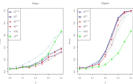
A difficulty in interpreting a dependogram is now illustrated with an example. Con-sider a model with three dependent variables Z(1),Z(2) and Z(3), where Z(1) and Z(2) are dependent, but the pair (Z(1), Z(2)) is independent of Z(3). Looking at Table 1 with the true characteristic functions, one can verify that µ12 6≡0, µ13 ≡0, µ23≡0, and µ123 ≡0. Therefore, only the test for the subset {1,2} is expected to be significant. The test for the subset {1,2,3} is not expected to be significant even though the three variables are dependent. Of course, the global test is expected to be significant as it will combine tests for all subsets.
8. Tests of Serial Independence
and
Zk = (Z
(1)
k , . . . , Z
(p)
k ) = (Yk, Yk+1, . . . , Yk+p−1), k = 1, . . . , n, (20) where Zk(j) =Yk+j−1, j = 1, . . . , p. Let f(t(1), . . . , t(p)) be the joint characteristic function of Z1 = (Y1, . . . , Yp) and f(B) be the joint characteristic function of Z1(B) = (Yj : j ∈ B).
For example, if p = 4 and the indices in the subsetB ={1,2,3} are translated by one to yield C =B+ 1 ={2,3,4} then, f(B) and f(C) are the same characteristic function since the process is stationary. In the serial context, a subset B and its translate, say B +k, can be treated as the same subset. The set Ip is thus reduced to Bp = {B ∈ Ip : 1 ∈ B}
and has now cardinality 2p−1−1. For a given B ∈ B
p, the M¨obius transformation of the
characteristic function f for the set B is given by
µB,s(t(B)) =
X
C⊆B
(−1)|B\C|f(C)(t(C)) Y
j∈B\C
f(1)(t(j)).
The subscript sstands for serial. The M¨obius transformation characterizes the serial inde-pendence: Y1, . . . , Yp are mutually independent if and only if,µB,s(t(B)) = 0, for allB ∈ Bp,
and all vectorst(B).
The corresponding process in the serial case is denotedRnB,sand is defined exactly as in
(2). Here, the index set of the processRnB,s is the Euclidean spaceRdB, whered
B=d1|B|.
Note that all the empirical characteristic functionsfn(j),j= 1, . . . , p, are now essentially the
same estimate of the unknown characteristic functionf(1). They are not replaced by a single estimate based on all nobservations to preserve the representation of the functional (8) in terms of doubly-centered matrices. The dependence statistic for the subsetB is now defined as the functional
WnB,s =
1 n
Z
|RnB,s(t(B))|2
Y
j∈B
dw(t(j)).
It can be computed as before in (8). Due to the stationarity, it should be noted that the same kernel is used to define the elements a(klj), for all j ∈ B. Two types of weighting measures are considered.
1. For HSIC, dw(t(j)) =dG(t(j)) is a probability measure with characteristic function ϕin which case
akl(j)=ϕ(Zk(j)−Zl(j)). (21) The dependence statistic is denotedWnB,s=H2nB,s. As in Theorem 2, the population
Hilbert-Schmidt independence criterion
H2
B,s=
Z
|µB,s(t(B))|2
Y
j∈B
dG(t(j))
is consistently estimated by H2
nB,s. The proof is omitted since it can be proven
as Theorem 2 using the ergodic theorem. The special case when dG(t(j)) is the probability measure of the stable distribution of index α is denoted H2(nB,sα), for α ∈
2. For distance covariance,dw(t(j)) =hC(d1, α)|t(j)|d1+α d1
i−1
, in which casea(klj)=−|Zk(j)− Zl(j)|α
d1. Under an appropriate moment condition as in Theorem 4, the consistency and weak convergence of the functional, which is denoted WnB,s = VnB,s2(α) for α ∈ (0,2),
should hold.
Pinkse (1998) proposed a non parametric test based on characteristic functions of serial independence against serial dependence of fixed lag k that is consistent against all such alternatives. It is based on a consistent estimator for an upper bound ofH2
B,sfor the subset
B ={1,1 +k}. The control of the global significance level when multiple tests are done for several values ofkis not addressed by this author. Diks and Panchenko (2007) constructed a test based on divergence measures between distributions using kernel-based quadratic forms to detect dependence at lag k using the subset B = {1,1 +k, . . . ,1 + (c−1)k} of given cardinality c. Their criterion is written as Q = Q11−2Q12+Q22. They used U-statistics as estimates for each term. Unfortunately, an error in the estimates of the last two terms on p. 85 leads to an erroneous statistic. If V-statistics are used instead, it is not hard to verify that their test statistic is of the exact form (17).
Under the hypothesis of serial independence, the vectors Zk = (Yk, Yk+1, . . . , Yk+p−1), k = 1, . . . , n, are dependent due to some overlapping Y’s. The proof of Theorem 5 is not directly applicable. Nevertheless, a very similar weak convergence theorem still holds.
Theorem 7 Let Y1, Y2, . . . be independent and identically distributed. Then, for any fixed
p, the process RnB,s ⇒ SB in C(RdB,C) to a zero mean complex Gaussian processes SB
with complex covariance function
E h
SB(t(B)) ¯SB(s(B))
i = Y
j∈B
h
f(1)(t(j)−s(j))−f(1)(t(j))f(1)(−s(j))i.
Moreover, the collection of processes (RnB,s : B ∈ Bp) ⇒ (SB : B ∈ Bp) on the product
of spaces ×
B∈BpC(R
dB,C) to a zero mean Gaussian process such that the marginal processes
SB, B ∈ Bp, are mutually independent.
In the next theorem, the asymptotic distribution of nH2
nB,s is described. The proof is
omitted since it is the same as for Theorem 6.
Theorem 8 Let WnB,s =HnB,s2 . If Y1, Y2, . . . are independent and identically distributed,
then nWnB,s ⇒ WB,s for each B ∈ Bp, where WB,s =
R
|SB(t(B))|2
Q
j∈BdG(t(j)).
More-over, the collection of variables(nWnB,s: B∈ Bp)⇒(WB,s: B ∈ Bp), where the variables
WB,s, B∈ Bp, are mutually independent.
The distribution of WB,s can be also represented using the Karhunen-Lo`eve expansion.
Without loss of generality, let B ={1, . . . , k}. Then, WB,s is distributed as in (15), where
the eigenvalues λ(1j), λ(2j), . . . no longer depend on j, but only on the probability measure P(1) of Y
1 and the weighting probability measure dG(t(1)). The eigenvalues λ1, λ2, . . . are those of the integral operator
Sk˜g(s(1)) = Z
Rd1 ˜
wherek(s(1), t(1)) =ϕ(t(1)−s(1)) is the translation invariant kernel (21) and ˜
k(s(1), t(1)) =k(s(1), t(1))−Ek(Y1, t(1))−Ek(s(1), Y2) +Ek(Y1, Y2),
for Y1, Y2 independent and distributed according to P(1), is the corresponding doubly-centered kernel.
Computations of p-values of individual tests and global tests in Sections 5 and 6 can also be used for testing for serial independence. Subsets B are now restricted to B ∈ Bp.
A modification to the dependogram is necessary since the null distributions of statistics of the same cardinality are now identical. The critical values cπB of Section 7 for all B of
the same cardinality are replaced by a single critical value as in Figure 6. Since there are
p−1
ω−1
subsets B containing 1 and of cardinalityω, the single critical value is taken as the π-quantile of the amalgamated N ωp−−11
statisticsWnB,i, fori= 1, . . . , N and|B|=ω.
It has been shown how distance covariance and HSIC tests can be adapted for testing for serial independence. The global testJ2
n in (17) can also be used for serial independence
by defining subsequences of lengthp as in (20).
9. Computational Aspects
The complexity cost of all randomization tests based on the M¨obius decomposition in this paper are of the orderO(n2rN), wherenis the sample size, r=Pq
i=2
p i
is the number of subsets considered in a global test of orderq, andN is the number of randomized samples. Even for the smallest value q = 2, the number of subsets of the order r =O(p2) increases quadratically with p. These tests thus become rapidly infeasible as n or p increases. The serial statistics in Section 8 have a lower complexity cost since in this caser =Pq
i=2
p−1
i−1
yields a number of subsets of the orderr =O(p) increasing linearly with pwhen q= 2. The statistics H2(nBα) and VnB2(α) are combined as in Section 6 to yield global statistics H2(nα) andVn2(α), respectively. Scale parametersβj in (10) must be selected forH2(nBα). They
are set to
βj =cj/medk<l|Zk(j)−Zl(j)|dj, j = 1, . . . , p. (22)
The choice cj = 1 leads to the so-called heuristic method suggested by Gretton et al.
(2008). Selection of very small constantscj allows to check the equivalence between distance
covariance and HSIC tests as described in (13). Unless stated otherwise, the heuristic method will be used forHSIC tests. Distance covariance andHSIC tests will be compared to two other tests: the test of Kojadinovic and Holmes (2009) denotedKH2
n for the mutual
independence case, or Kojadinovic and Yan (2011) denoted KY2
n for the serial case, and
the testJn2(2) in (17) with heuristic scale parameters (22) as in Sejdinovic et al. (2013a).
When dj = 1 for all j = 1, . . . , p, the statistics KHn2 (or KYn2) are replaced by the
equivalent statistic of Genest and R´emillard (2004) denotedGR2
n. KHn2 differs from GR2n
only in the approximation used forp-values. The former uses a randomization test, whereas the latter takes advantage of the fact that fordj = 1, the test is distribution free implying
that critical values can be obtained by simulating the null distribution for given values of nand p. Thus, a single set of critical values can be used for all replicates.
The copula R package (Kojadinovic and Yan, 2010) functions multIndepTest and
multSerialIndepTest were used for tests based on KH2
Inci-dentally, the implementation of KH2
n unnecessarily recomputes the doubly-centered
matri-ces A(j) for every permutation in their C subroutine bootstrap MA I. The same package also contains the functions indepTest and serialIndepTest for GR2
n. An R function
for distance covariance and HSIC tests proposed in this paper for p ≥ 2 is available at
dms.umontreal.ca/~bilodeau. For p = 2, it produces, up to a factor of 1/n depending on the definitions of statistics, the same result as the function dcov.test of the energy
package (Rizzo and Szekely, 2016). Computations in Section 10 were done on an Intel(R) Core(TM) i7 with a CPU of 3.20 GHz.
10. Simulated Models
All empirical significance levels and empirical powers in this section are evaluated with 1000 tests (replicates) conducted at a global significance level α0 = 0.05. The p-values of all randomization tests are based on 1000 permutations (the default). Power results are summarized by graphics with a tick mark at 0.05 on the power axis to check for the conformity of empirical significance levels to the nominal level. Six tests are compared: distance covariance testsVn2(1/2) andVn2(1),HSIC testsH2(1n /2) and H2(1)n , the test KHn2 of
Kojadinovic and Holmes (2009) and the testJn2(2) in (17). When alldj = 1, the testKHn2
is replaced by GR2
n as explained in Section 9. Also, for the serial case, the test KHn2 is
replaced by the testKY2
n of Kojadinovic and Yan (2011). Unless stated otherwise,p-values
of tests based on the M¨obius decomposition are combined using the method of Fisher.
10.1 Copula Models
Power comparisons are made for the Gaussian, Student, Frank and Clayton copulas. A general reference for copulas is the book by Nelsen (2006).
10.1.1 Gaussian and Student Copulas with Bivariate Marginals
As in Kojadinovic and Holmes (2009), a correlation matrix is constructed of the form
R=
(1−ρw)I2+ρwJ2J20 ρbJ2J20 ρbJ2J20 ρbJ2J20 (1−ρw)I2+ρwJ2J20 ρbJ2J20 ρbJ2J20 ρbJ2J20 (1−ρw)I2+ρwJ2J20
, (23)
where I2 is the identity matrix of dimension 2 and J2 is the vector of ones of dimension 2. Notationsw and b stand for within and between, respectively. Samples of size n= 100 are generated from a multivariate distribution of dimension 6 (Gaussian or Student with 2 degrees of freedom) with correlation matrix R in (23). Probability transforms are then applied so that all 6 variables are uniformly distributed on the interval (0,1). The resulting vector is partitioned into three two-dimensional vectors. The value of ρw is set to 0.5.
For the Gaussian model, Figure 1 shows that the best test is KH2
n followed closely by
Vn2(1). However, for the Student model, KHn2 performs poorly compared to all the other
tests, the most powerful test being H2(1n /2). For the Student model, the three components
are always dependent even when ρb = 0 which explains the power at ρb = 0 in the right
0.00 0.05 0.10 0.15 0.20 0.25
0.0
0.2
0.4
0.6
0.8
1.0
Gaussian
ρb
P
o
w
er
Vn2(1/2)
Vn2(1)
H2(1n/2)
H2(1)n
KH2
n
Jn2(2)
0.00 0.05 0.10 0.15 0.20 0.25
0.0
0.2
0.4
0.6
0.8
1.0
Student
ρb
P
o
w
er
Vn2(1/2)
Vn2(1)
H2(1n/2)
H2(1)n
KH2
n
Jn2(2)
Figure 1: Empirical powers for the Gaussian (left panel) and Student (right panel) copulas with bivariate marginals of Section 10.1.1.
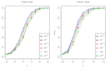
10.1.2 Frank and Clayton Copulas with Univariate Marginals
The Frank and Clayton copulas are now considered for n = 100, p = 3 and dj = 1 for
j= 1,2,3. These two copulas have a parameterθwith the valueθ= 0 corresponding to the independence copula. For the Frank copula, independence is obtained as the limiting case θ → 0. Figure 2 shows that for both copulas, the tests GR2
n and V
2(1)
n have very similar
powers and are the most powerful. The least powerful test isJn2(2). TheHSICtests are less
powerful than their distance covariance counterparts, but their powers could be increased to those of distance covariance by selecting smaller scale parameters as predicted by (13).
10.1.3 Frank Copula with Bivariate Marginals
The Frank copula model is now considered forp= 3 anddj = 2 forj= 1,2,3. The sample
0.0 0.5 1.0 1.5 2.0 2.5
0.0
0.2
0.4
0.6
0.8
1.0
Frank copula
θ
P
o
w
er
Vn2(1/2)
Vn2(1)
H2(1n/2)
H2(1)n
GR2
n
Jn2(2)
0.0 0.2 0.4 0.6 0.8
0.0
0.2
0.4
0.6
0.8
1.0
Clayton copula
θ
P
o
w
er
Vn2(1/2)
Vn2(1)
H2(1n/2)
H2(1)n
GR2
n
Jn2(2)
Figure 2: Empirical powers for the Frank (left panel) and Clayton (right panel) copulas with univariate marginals of Section 10.1.2.
10.2 Model of Romano and Siegel
The original model is taken from Kojadinovic and Holmes (2009) which extends an example in Genest and R´emillard (2004). Samples of sizen= 100 are generated from the distribution of a 12-dimensional random vector as follows.
1. Generate a two-dimensional Gaussian vectorX(1)= (X(1) 1 , X
(1)
2 ) with means 0, variances 1, and covariance 0.5.
2. Generate two independent copiesZ(2) andZ(3) of X(1). 3. DefineZ(1)= (Z(1)
1 , Z (1) 2 ) byZ
(1)
i =|X
(1)
i |sign(Z
(2) 1 Z
(3)
1 ),i= 1,2.
4. Generate a three-dimensional Gaussian vector Z(4) with means 0, variances 1, and co-variances 0.3.
5. Generate an independent copy X(5) of Z(4). 6. DefineZ(5)=Z(4)+X(5).
0.0 0.5 1.0 1.5
0.0
0.2
0.4
0.6
0.8
1.0
θ
P
o
w
er
Vn2(1/2)
V2(1)
n
H2(1/2)
n
H2(1)
n
KH2
n
Jn2(2)
Figure 3: Empirical powers for the Frank copula with bivariate marginals of Section 10.1.3.
in which the two three-dimensional vectors Z(4) and Z(5) are dependent. One can check that the only non null termsµB are for the subsets {4,5},{1,2,3}, and {1,2,3,4,5}.
In order to compare the powers of various tests, a modified model with weaker depen-dence is introduced. Items 3 and 6 are modified to
3’. Define Z(1) = (Z(1) 1 , Z
(1) 2 ) by Z
(1)
i = (1−θ)|X
(1)
i |+θ|X
(1)
i |sign(Z
(2) 1 Z
(3)
1 ),i= 1,2, 6’. Define Z(5) =θZ(4)+X(5),
for some θ ∈[0,0.4]. Mutual independence now holds among the 5 components for θ = 0 and the dependence increases with θ. The value θ= 1 leading to the original model is not considered since it yields a dependence too easily detected.
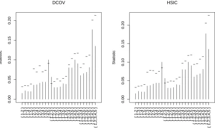
Figure 4 is the dependogram based on one simulated sample withθ= 0.4. The statistics computed areVnB2(1)andH
2(1)
nB with very small constantscj =.0001 in (22). It illustrates the
are generally higher because the presence of noise is less important than in subsets of large cardinality. Tests based on the M¨obius decomposition combine p-values according to the
0.00
0.05
0.10
0.15
0.20
DCOV
Statistic
− − −− −
− −
− − −
−− −−−−
− −
− −
−− − −
− −
{ 1,2 } { 1,3 } { 1,4 } { 1,5 } { 2,3 } { 2,4 } { 2,5 } { 3,4 } { 3,5 } { 4,5 }
{ 1,2,3 } { 1,2,4 } { 1,2,5 } { 1,3,4 } { 1,3,5 } { 1,4,5 } { 2,3,4 } { 2,3,5 } { 2,4,5 } { 3,4,5 } { 1,2,3,4 } { 1,2,3,5 } { 1,2,4,5 } { 1,3,4,5 } { 2,3,4,5 }
{ 1,2,3,4,5 }
0.00
0.05
0.10
0.15
0.20
HSIC
Statistic
− − −− − − − − −
−
− −− − − −
−− − −
− − −−
− −
{ 1,2 } { 1,3 } { 1,4 } { 1,5 } { 2,3 } { 2,4 } { 2,5 } { 3,4 } { 3,5 } { 4,5 }
{ 1,2,3 } { 1,2,4 } { 1,2,5 } { 1,3,4 } { 1,3,5 } { 1,4,5 } { 2,3,4 } { 2,3,5 } { 2,4,5 } { 3,4,5 } { 1,2,3,4 } { 1,2,3,5 } { 1,2,4,5 } { 1,3,4,5 } { 2,3,4,5 }
{ 1,2,3,4,5 }
Figure 4: Dependograms for one sample of sizen= 100 from the modified model of Romano and Siegel withθ= 0.4 in Section 10.2 based onVnB2(1)(left panel) andH2(1)nB (right panel) with small constantscj =.0001 in (22).
methods of Tippett and Fisher. Figure 5 shows that KH2
n is more powerful than distance
covariance and HSIC tests when using the method of Fisher. However, the method of Tippett is markedly more powerful than that of Fisher. This finding should not come as a surprise since only 3 of the 26 sub-hypotheses are false. Using the method of Tippett the most powerful test Vn2(1) is markedly better than Jn2(2) and KHn2. The popular belief that
the method of Fisher is more powerful than that of Tippett should not be given too much consideration. The preferred test depends on the model under consideration.
10.3 Bivariate AR(1) Model
The model considered is the bivariate AR(1) model defined by Yk=AYk−1+k, where the
innovationsk are independently distributed as bivariate Gaussian with mean vector 0 and
covariance matrixC. The final specification is made by defining
A=
0 θ θ 0
andC =
1 0.5 0.5 1
0.0 0.1 0.2 0.3 0.4
0.0
0.2
0.4
0.6
0.8
1.0
Fisher
θ
P
o
w
er
Vn2(1/2)
Vn2(1)
H2(1n/2)
H2(1)n
KH2
n
Jn2(2)
0.0 0.1 0.2 0.3 0.4
0.0
0.2
0.4
0.6
0.8
1.0
Tippett
θ
P
o
w
er
V2(1n /2)
V2(1)n
H2(1n/2)
H2(1)n
KH2
n
Jn2(2)
Figure 5: Empirical powers for the modified model of Romano and Siegel in Section 10.2. The methods of Fisher (left panel) and Tippett (right panel) are used to combine p-values.
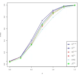
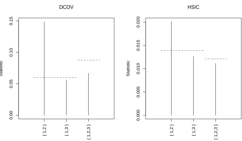
The serial dependence of the sequence increases with θ and serial independence holds for θ = 0. Tests of Tippett and Fisher are compared. The value p = 3 chosen arbitrarily can detect dependencies among three successive observations. In particular, it can detect dependencies at lags one or two. Sequences of length m = 100 are generated using the
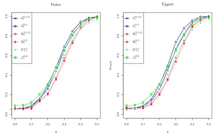
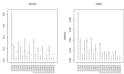
mAr.sim function of the R package mAr (Barbosa, 2012). The dependogram in Figure 6 shows a significant dependence at lag one. It shortly fails to detect the weaker dependence at lag 2 with the short sequence length of 100. Power functions in Figure 7 revealVn2(1) as
the most powerful test. Comparisons between Fisher and Tippett tests show comparable powers with a slight advantage for Tippett. Higher powers of Jn2(2) locally around θ = 0
can be attributed to the higher empirical significance level of this test.
11. Applications
0.00
0.05
0.10
0.15
DCOV
Statistic
{ 1,2 } { 1,3 }
{ 1,2,3 }
0.000
0.005
0.010
0.015
0.020
HSIC
Statistic
{ 1,2 } { 1,3 }
{ 1,2,3 }
Figure 6: Dependograms for one sequence of length m = 100 for the AR(1) model with θ= 0.4 of Section 10.3 based on VnB2(1) (left panel) and H
2(1)
nB (right panel).
11.1 Testing Mutual Independence Between Air Temperature, Soil Temperature, Humidity, Wind and Evaporation
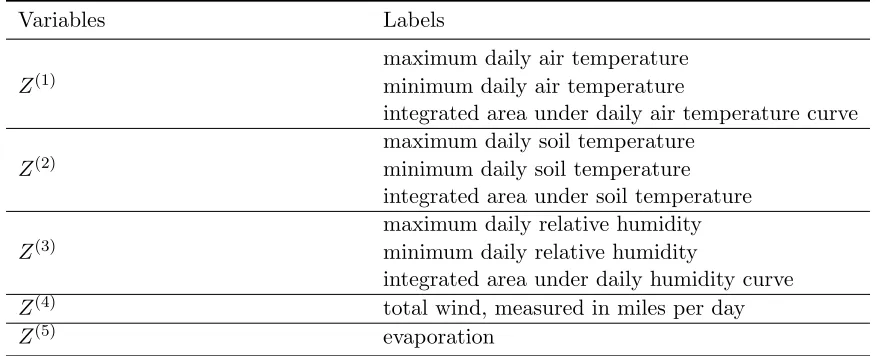
These meteorological data are from Rencher (1995, p. 294). Table 2 describes the data with 46 observations on 11 variables. When a data set consists of variables measured on different scales, the scaling of variables often helps to enhance the appearance of the dependogram. In this application, variables were scaled to zero mean and unit variance. TheRpackageMVN
0.0 0.1 0.2 0.3 0.4 0.5
0.0
0.2
0.4
0.6
0.8
1.0
Fisher
θ
P
o
w
er
Vn2(1/2)
Vn2(1)
H2(1n/2)
H2(1)n
KY2
n
Jn2(2)
0.0 0.1 0.2 0.3 0.4 0.5
0.0
0.2
0.4
0.6
0.8
1.0
Tippett
θ
P
o
w
er
V2(1n /2)
V2(1)n
H2(1n/2)
H2(1)n
KY2
n
Jn2(2)
Figure 7: Empirical powers for the AR(1) model of Section 10.3. The methods of Fisher (left panel) and Tippett (right panel) are used to combinep-values.
However, wind does not exhibit any dependence of order 2 or 3 with any of the other 4 groups of variables.
11.2 Testing Serial Independence for Financial Data
Tests of serial independence of the three dimensional sequence formed by the daily percent increasing rates (DPIR) of indices from three stock markets: S&P/TSX composite (TSX), DOW JONES and S&P500. The values of indices are taken at closure. The series of length 534 range from January 2, 2014 to March 2, 2016. Note that five index values are observed weekly since the stock exchanges are not opened on weekends. The top row of Figure 9 shows that the financial series considered are not stationary. It is more appropriate to consider DPIR values. In the bottom row, one may see that DPIR values are more stationary, although still not perfectly stationary.
Tests of serial independence KY2
nB, V
2(1)
nB , and the test of non serial correlation V
2(2)
nB
are conducted on the 3 joint series. The value of p= 10 allows a maximum lag of 9 days. Figure 10 reveals dependencies at small lags of 1, 2, and 4 in the dependogram of VnB2(1).
The dependogram of KY2
nB was produced with the copula package and does not include
critical values. Nevertheless, KY2
nB and V
2(1)
Variables Labels
maximum daily air temperature Z(1) minimum daily air temperature
integrated area under daily air temperature curve maximum daily soil temperature
Z(2) minimum daily soil temperature integrated area under soil temperature maximum daily relative humidity Z(3) minimum daily relative humidity
integrated area under daily humidity curve Z(4) total wind, measured in miles per day
Z(5) evaporation
Table 2: Variables related to air temperature, soil temperature, humidity, wind and evap-oration.
at lag 4. The distance covarianceVnB2(2) of index 2 was also performed on the sequence. One should recall that VnB2(2) is no longer a test of serial independence, but merely of non serial
correlation. Interestingly, this test did not reveal any significant serial correlation. In an attempt to unravel the most significant dependency at lag 4 declared by VnB2(1), Figure 11 is a scatterplot of DPIR values observed on day k and k+ 4 for the TSX market. The Pearson (p-value of 0.11) and the Kendall (p-value of 0.14) correlation tests applied to this scatterplot are not significant. The test VnB2(1) for B ={1,5} on the single TSX market is very significant (p-value less than 0.001). A broken line regression with a change point at the origin was fitted to this scatterplot to account for different regimes according to whether DPIR is negative or positive. This regression model has three parameters for the intercept and slopes at the left and right of the origin. The left slope is very significant (p-value of 0.000015) contrary to the right slope (p-value of 0.021). The very significant left slope could be interpreted by the tendency of the TSX market to recover in the days following a decline. The sharper the market declines, the stronger it recovers. Among days such that DPIRk < ξ, the percentage of days with DPIRk+4 > 0 is 60.7% for ξ = −0.5. This percentage goes up to 63.4% for ξ = −1 and to 68.2% for ξ = −1.5. Similar conclusions were found for the DOW JONES and S&P500 stock markets.
12. Conclusion
Generalizations of distance covariance and HSIC tests were done successfully. For both mutual and serial independence hypotheses, the dependence statistics related to distance covariance and HSIC were defined using the M¨obius transformation. Simple and explicit expressions for dependence statistics were derived in the explicit form (8) as a sum over all elements of a componentwise product of doubly-centered matricesA(j)= (A(j)
kl).