Determinantal Point Processes for Coresets

Determinantal Point Processes for Coresets

Nicolas Tremblay [email protected]

Simon Barthelm´e [email protected]

Pierre-Olivier Amblard [email protected] CNRS, Univ. Grenoble Alpes, Grenoble INP, GIPSA-lab, Grenoble, France

Editor:Michael Mahoney

Abstract

When faced with a data set too large to be processed all at once, an obvious solution is to retain only part of it. In practice this takes a wide variety of different forms, and among them “coresets” are especially appealing. A coreset is a (small) weighted sample of the orig-inal data that comes with the following guarantee: a cost function can be evaluated on the smaller set instead of the larger one, with low relative error. For some classes of problems, and via a careful choice of sampling distribution (based on the so-called “sensitivity” met-ric), iid random sampling has turned to be one of the most successful methods for building coresets efficiently. However, independent samples are sometimes overly redundant, and one could hope that enforcing diversity would lead to better performance. The difficulty lies in proving coreset properties in non-iid samples. We show that the coreset property holds for samples formed with determinantal point processes (DPP). DPPs are interest-ing because they are a rare example of repulsive point processes with tractable theoretical properties, enabling us to prove general coreset theorems. We apply our results to both thek-means and the linear regression problems, and give extensive empirical evidence that the small additional computational cost of DPP sampling comes with superior performance over its iid counterpart. Of independent interest, we also provide analytical formulas for the sensitivity in the linear regression and 1-means cases.

Keywords: Coresets, Determinantal Point Processes, Sensitivity

1. Introduction

Given a learning task, if an algorithm is too slow on large data sets, one can either speed up the algorithm or reduce the amount of data. The theory of “coresets” gives theoretical guarantees on the latter option. A coreset is a weighted sub-sample of the original data, with the guarantee that for any learning parameter, the task’s cost function estimated on the coreset is equal to the cost computed on the entire data set up to a controlled relative error.

An elegant consequence of such a property is that one may run learning algorithms solely on the coreset, allowing for a significant decrease in the computational cost while guaranteeing almost-equal performance. There are many algorithms that produce coresets, with some tailored for a specific task (such as k-means, k-medians, logistic regression, etc.), and others more generic. Also, there exists coreset sampling strategies both for the streaming setting and the offline setting: we choose here to focus on the offline setting. We

c

follow the review of Munteanu and Schwiegelshohn (2017) and classify coreset construction techniques in four categories:

1. Geometric decompositions (e.g.,Har-Peled and Mazumdar, 2004; Har-Peled and Kushal, 2005; Agarwal et al., 2005; Har-Peled, 2011). These methods propose to first discretize the ambient space of the data into a set of cells, snap each data point to its nearest cell in the discretization, and then use these weighted cells to approximate the target tasks. In all these constructions, the minimum number of samples required to guaran-tee the coreset property depends exponentially in the dimensionality of the ambient space, making them less useful in high-dimensional problems.

2. Gradient descent (e.g., Badoiu and Clarkson, 2008; de la Vega et al., 2003; Kumar et al., 2010; Clarkson, 2010). These methods have been originally designed for the smallest enclosing ball problem (i.e., finding the ball of minimum radius enclosing all datapoints), and have been later generalized to other problems. One of the main drawback of these algorithms in thek-means setting for instance is that their running time grows exponentially in the number of classesk(Kumar et al., 2010). Also, these algorithms provide only so-called weak coresets.

3. Random sampling (e.g., Chen, 2009; Langberg and Schulman, 2010; Feldman and Langberg, 2011; Braverman et al., 2016; Bachem et al., 2017). The state of the art for many different tasks such ask-means ork-median is currently via iid random non-uniform sampling. For optimal performance, the probability to sample an element should be set proportional to a quantity known as itssensitivity (introduced by Lang-berg and Schulman (2010)). See Definition 2 for the formal definition of sensitivity. In practice, it is unpractical to compute sensitivities: state of the art algorithms rely on bi-criteria approximations to find upper bounds, and set the probability distribu-tion propordistribu-tional to this upper bound. More details on these results are provided in Section 2.4.

4. Sketching and projections (e.g.,Phillips, 2016; Woodruff, 2014; Mahoney, 2011; Bout-sidis et al., 2015; BoutBout-sidis and Gittens, 2013; Cohen et al., 2015; Keriven et al., 2017; Clarkson and Woodruff, 2017; Becchetti et al., 2019). Another direction of research regarding data reduction that provably keeps the relevant information for a given learning task is via sketches (Woodruff, 2014): compressed mappings (obtained via projections) of the original data set that are in general easy to update with new or modified data. Sketches are not strictly speaking coresets, and the difference resides in the fact that coresets are subsets of the data, whereas sketches are projections of the data. Note finally that the frontier between the two is permeable and some data summaries may combine both.

negatively correlated point processes, i.e., point processes for which sampling jointly two similar datapoints is less probable than sampling two very different datapoints. Methods based on negatively correlated sampling have been studied in the past for specific tasks.

For instance, for the column subset selection problem (CSSP), a method called volume sampling has been investigated in the literature (see Deshpande et al., 2006; Deshpande and Rademacher, 2010). A determinant-based sampling strategy has also been studied by Be-labbas and Wolfe (2009). Also, a recent work (Belhadji et al., 2018) discusses with some details the different existing sampling-based methods (iid or with negative correlations) for the CSSP, and compares them versus a determinantal sampling strategy. Another spe-cific task for which volume sampling strategies have been used is linear regression (see for instance Derezinski et al., 2018; Derezinski and Warmuth, 2018).

We propose: i/ to concentrate on a specific type of negatively-correlated sampling: determinantal point processes (DPPs), known to provide samples that are representative of the “diversity” in the data set (Kulesza and Taskar, 2012); ii/ to study their coreset performance on generic tasks. To the best of our knowledge, we provide the first general coreset guarantee using non-iid random sampling.

DPPs are parametrized by a positive semi-definite matrix calledL-ensemble and denoted by L. This matrix encodes for the inclusion probabilities of each sample as well as higher order inclusion probabilities defining the correlation between samples. Note that DPPs have in general a random number of samples which in many practical situations is not adapted. This lead Kulesza and Taskar (2012) to define m-DPPs: DPPs conditioned to output m samples (for precise definitions related to DPPs and m-DPPs, see Section 2.6). It so happens that DPPs are more tractable than m-DPPs, making some proofs easier to show in the DPP context; however, m-DPPs are more useful in practice, especially when one needs to compare with fixed-size sampling methods as we do in this work. The reader should thus be mentally prepared to juggle from one concept to the other throughout the remainder of this paper.

1.1. Contributions

Theoretical contributions. Our theorems are quite generic, and assume mostly that the cost functions under study are Lipschitz. We have two main lines of argument: the first is that DPP samples do indeed verify the coreset property, the second is that DPPs produce

better coresets than their iid counterparts if one uses the right L-ensemble to define the DPP. More specifically, we show:

• Theorem 8 and 20. Whatever the higher-order inclusion probabilities, if the inclusion probability of each sample of a DPP (orm-DPP) is set proportional to the sensitivity, then the results are at least as good as in the iid case. Technical limitations in controlling the concentration properties of correlated samples currently keep us from deriving exactly the minimum coreset size one may hope for when using DPPs.

• Theorem 12 and its Corollary 14. In the fixed-size context: a sample from anm-DPP with a rank m projective L-ensemble (also called projective DPP) necessarily leads to a lower variance than its iid counterpart with same inclusion probabilities.

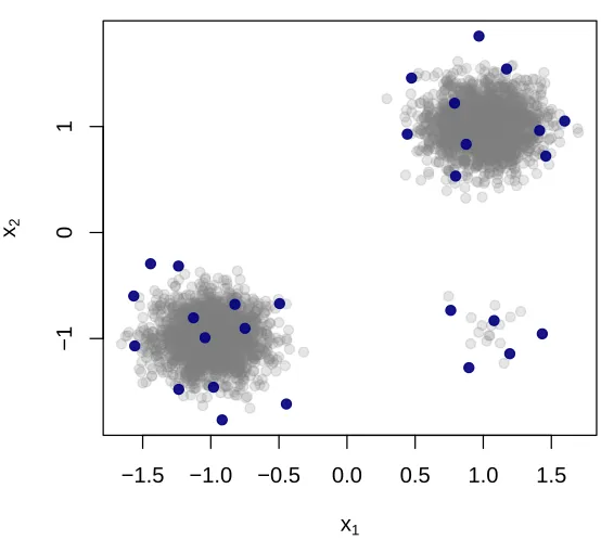
We also show Theorem 16, stating that samples from a particular polynomialL-ensemble based on the Vandermonde matrix of the data asymptotically have a rebalancing property, made precise in Section 3.3. For instance in thek-means setting, this rebalancing property means that, asymptotically, such a DPP produces samples in each cluster, even if some are much smaller than others (see Figure 1 for an illustration).

Finally, of independent interest, we provide for the first time analytical formulas for the sensitivity, in two specific settings: the 1-means and the linear regression cases (Lemmas 23 and 25).

Empirical contributions. In the iid setting, for optimal performance, the probability of sampling an element should be set proportional to its sensitivity. In general, the sensitivity is not computable in polynomial time, thus out of reach in practice. For the specific 1-means and linear regression tasks, now that we have provided analytical formulas, these quantities become computable in polynomial time but turn out to be heavier to compute than solving the task on the whole data set –thus useless in practice. The usual workaround in the iid setting is to set the sampling probability proportional to an upper bound (efficiently com-puted via, e.g., bi-criteria approximations) of the sensitivity. Thankfully, one still controls the performance of the obtained coreset (as a function of the upper bound’s tightness).

Sensitivity playing a central role in the DPP-based coreset theorems we provide, these theorems also suffer from the same impracticality. Unfortunately, due to the dependencies introduced by DPPs, mere upper bounds of the sensitivity are not sufficient to propose a controlled workaround. The theorems enable to discuss in some detail what is the ideal task-specific choice ofL-ensemble, but in practice we for now need to resort to heuristics.

We apply our results to both the k-means and the linear regression problems where the initial data consists in n points in Rd. As explained, the ideal choice of L-ensemble L for DPP sampling is untractable in practice, we thus provide two efficient heuristics: one based on random Fourier features of the Gaussian kernel, the other on polynomial features. We pay particular attention to the computation cost of these two heuristics, and provide implementation details. These heuristics output a coreset sample in respectively

O(nm2+nmd) and O(nm2) time wherem is the number of samples of the coreset. In the

k-means context, this is to compare to O(nkd) the cost of the current state of the art iid

sampling algorithm via bi-criteria approximation. m being necessarily larger than dand k to obtain the coreset guarantee in this context, our proposition is computationally heavier, especially as m increases. We provide nonetheless extensive empirical evidence showing that this additional cost stays reasonable, given the enhanced performance it provides. In particular, given that we provide analytical formulas for the sensitivities in the 1-means and linear regression contexts, we are able, in these two settings, to compare the DPP-based heuristics to the ideal iid coresets (i.e., the coresets sampled iid from the distribution

Finally, a Julia toolbox called DPP4Coresets is available on the authors’ website.1

1.2. Organization of the paper

The paper is organized as follows. Section 2 recalls the background: the types of learning problems under consideration, the formal definition of coresets, sensitivities and DPPs. The theoretical Section 3 presents our main theorems on the performance of DPPs for coreset sampling: while Section 3.1 details coreset performance in the usual formulation of coreset theorems, Section 3.2 shows general variance arguments in favor of DPPs, and finally Section 3.3 provides an original asymptotic rebalancing property of DPPs. Section 4.1 shows how these theorems are applicable to both thek-means and the linear regression problems. We provide in Section 5 a discussion on the choice ofL-ensemble adapted to these problems, and detail our sampling algorithms. Finally, the empirical Section 6 presents experiments on artificial as well as real-world data sets comparing the performance of DPP sampling to iid sampling. Section 7 concludes the paper. Note that for the sake of readability, many proofs and some implementation details are pushed to the Appendix.

2. Background

LetX ={x1, . . . ,xn}be a set ofndatapoints. Let (Θ, dΘ) be a metric space of parameters,

and θan element of Θ. We consider cost functions of the form:

L(X, θ) = X

x∈X

f(x, θ), (1)

wheref is a non-negativeγ-Lipschitz function (γ >0) with respect to θ,i.e.,∀x∈ X:

∀θ∈Θ f(x, θ)≥0,

∀(θ, θ0)∈Θ2 |f(x, θ)−f(x, θ0)| ≤γ dΘ(θ, θ0).

Many classical machine learning cost functions fall under this model: k-means, k-median, logistic or linear regression, support-vector machines, low-rank approximations of matrices, etc.

2.1. Problem considered

A standard learning task is to minimize the costL over all θ∈Θ. We write:

θopt= argmin θ∈Θ

L(X, θ), Lopt=L(X, θopt) and hfiopt =

Lopt

n . (2)

In some instances of this problem, e.g., if n is very large and/or if f is expensive to evaluate and should be computed as rarely as possible, one may rely on sampling strategies to efficiently perform this optimization task.

2.2. Coresets

Let S = {xs1, . . . ,xsm} be a subset of X (possibly with repetitions). To each element xs ∈ S, associate a weight ω(xs) ∈ R+. Define the estimated cost associated to the

weighted subsetS as:

ˆ

L(S, θ) = X

xs∈S

ω(xs)f(xs, θ). (3)

Definition 1 (Coreset) Let ∈(0,1). The weighted subset S is a -coreset for L if, for any parameterθ, the estimated cost is equal to the exact cost up to a relative error:

∀θ∈Θ

ˆ L

L−1

≤. (4)

This is the so-called “strong” coreset definition, as the -approximation is required for all θ∈Θ. A weaker version of this definition exists in the literature where the-approximation is only required for θopt. In the following, we focus on theorems guaranteeing the strong coreset property.

Let us write ˆθopt the optimal solution computed on the weighted subset S: ˆθopt = argmin_θ∈ΘL(ˆ S, θ). An important consequence of the coreset property is the following:

(1−)L(X, θopt)≤(1−)L(X,θˆopt)≤L(ˆ S,θˆopt)≤L(ˆ S, θopt)≤(1 +)L(X, θopt),

i.e., running an optimization algorithm on the weighted sample S will result in a minimal learning cost that is a controlled -approximation of the learning cost one would have ob-tained by running the same algorithm on the entire data set X. Note that the guarantee is over costs only: the estimated optimal parameters ˆθopt and θopt may be different. Nev-ertheless, if the cost function is well suited to the problem: either there is one clear global minimum and the estimated parameters will almost coincide; or there are multiple solutions for which the learning cost is similar and selecting one over the other is not an issue.

In terms of computation cost, if the sampling scheme is efficient, nis very large and/or f is expensive to compute for each datapoint, coresets thus enable a significant gain in computing time.

2.3. Sensitivity

To define appropriate sampling schemes for coresets, Langberg and Schulman (2010) intro-duce the notion of sensitivity:

Definition 2 (Sensitivity) The sensitivity of a datapointxi ∈ X with respect to a fuction f :X,Θ→R+ is:

σi= max θ∈Θ

f(xi, θ)

L(X, θ) ∈[0,1]. (5)

Also, the total sensitivity is defined as :

S= n

X

i=1

Note that the fraction defining the sensitivity is not defined for L(X, θ) = 0 (that may happen for instance in the 1-means problem, in the degenerate case where allxi are super-imposed and equal toθ). For simplicity, we suppose that ∀θ∈Θ, L(X, θ)>0.

The sensitivity is related to the concept of statistical leverage score (e.g., Drineas and Mahoney, 2018; Drineas et al., 2012), which plays a crucial role in iid random sampling theorems in the randomized numerical linear algebra literature (Mahoney, 2011). Both notions are similar, but not equivalent. For instance, we show in Lemma 25 that sensitivities for the linear regression task are different from the usual definition of leverage score in this context. Thus, in general, leverage scores used in the randomized linear algebra literature are not sensitivities,i.e., they do not necessarily verify Eq. (5).

In words, the sensitivity σi is the worse case contribution of datapoint xi in the total cost. Informally, the larger it is, the larger its “outlierness” (Lucic et al., 2016).

2.4. iid importance sampling and state of the art results

In the iid sampling paradigm, the importance sampling estimator of L is the following. Say the sample set S consists in m samples drawn iid with replacement from a (discrete) probability distribution p∈Rn (with pi the probability of samplingxi at each draw, and

P

ipi = 1). Denote by i the random variable counting the number of occurences of xi in

S. One may define ˆLiid, the so-called importance sampling estimator ofL, as :

ˆ

Liid(S, θ) =

X

i

f(xi, θ)i mpi

. (6)

One can show that E(i) =mpi, such that ˆLiid is an unbiased estimator of L: E( ˆLiid(S, θ)) =L(X, θ).

The concentration of ˆLiid around its expected value is controlled by the following state

of the art theorem:

Theorem 3 (Coresets with iid random sampling) Let p∈[0,1]n be a probability dis-tribution over all datapoints X with pi the probability of sampling xi and Pipi = 1. Draw m iid samples with replacement according to p. Associate to each sample xs a weight ω(xs) = 1/mps. The weighted subset obtained is a -coreset with probability1−δ provided

that:

m≥m∗

with

m∗ =O 1

2

max i

σi pi

2

(d0+ log (1/δ))

!

,

whered0 is the pseudo-dimension of Θ(a generalization of the Vapnik-Chervonenkis dimen-sion). The optimal probability distribution minimizing m∗ is pi =σi/S. In this case, the

weighted subset is a -coreset with probability1−δ provided that:

m≥ O

S2 2 (d

0_{+ log (1/δ))}

For instance, in the k-means setting2, d0 = dklogk and S = O(k) such that the coreset property is guaranteed with probability 1−δ provided that:

m≥ O

k2

2(dklogk+ log (1/δ))

.

This theorem is taken from the paper by Bachem et al. (2017). Its original form goes back to Langberg and Schulman (2010). Note that sensitivities cannot be computed rapidly, such that, as it is, this theorem is unpractical. Thankfully, bi-criteria approximation schemes (such as Algorithm 2 of Bachem et al. 2017, or other propositions such as in Feldman and Langberg 2011; Makarychev et al. 2016) may be used to efficiently find an upper bound of the sensitivity for all i: bi ≥ σi. Noting B = Pbi, and setting pi = bi/B, one shows that the coreset property may be guaranteed in the iid framework provided that

m≥ OB2

2(d

0_{+ log (1/δ)).}

Note that if one authorizes coresets with negative weights (that is, authorizes nega-tive weights in the estimated cost of Eq. (3)), then the above theorem may be further improved (Feldman and Langberg, 2011). Nevertheless, we prefer to restrict ourselves to positive weights as optimization algorithms such as Lloyd’sk-means heuristics (Lloyd, 1982) are in practice more straightforward to implement on positively weighted sets rather than on sets with possibly negative weights.

Finally, Braverman et al. (2016, Theorem 5.5) improve the previous theorem by showing that under the same non-uniform iid framework, the coreset property is guaranteed provided thatm≥ O S

2(d

0_{logS+ log (1/δ))}

, thus reducing the term in S2 toSlogS.

2.5. Correlated importance sampling

Eq. (6) is not suited to correlated sampling and, in the following, we will use a slightly different importance sampling estimator, more adapted to this case. Consider a point process defined onX that outputs a random sampleS ⊂ X. For each data pointxi, denote by πi its inclusion (or marginal) probability:

πi =P(xi ∈ S). (7)

Moreover, denote by i the random Boolean variable such that i = 1 if xi ∈ S, and 0 otherwise. In this paper, we focus on the following definition3 of the importance sampling cost estimator ˆL:

ˆ

L(S, θ) =X i

f(xi, θ)i πi

. (8)

By construction,E(i) =πi, such that ˆL is an unbiased estimator ofL:

E( ˆL(S, θ)) =L(X, θ).

2. In the literature (Feldman and Langberg, 2011; Balcan et al., 2013),d0 is often taken to be equal todk

in thek-means setting. We nevertheless agree with Bachem et al. (2017) and their discussion in Section 2.6 regardingk-means’ pseudo-dimension and thus writed0=dklogk

3. Note that in fact ˆLiidand ˆLare the same objects if one definesito be the number of timesiis sampled (which will be in practice Boolean in the DPP case as the same sample can never be sampled twice in this context) and write ˆL(S, θ) =P

i f(xi,θ)i

Studying the coreset property in this setting boils down to studying the concentration properties of ˆLaround its expected value.

2.6. Determinantal Point Processes

In order to induce negative correlations within the samples, we choose to focus on Deter-minantal Point Processes (DPP), point processes that have recently gained attention due to their ability to output “diverse” subsets within a tractable probabilistic framework (for instance with explicit formulas for marginal probabilities). In the following, 2[n] denotes the set of all possible subsets of thenfirst integers.

The central object is called the L-ensemble, and is nothing else than a positive semi-definite matrixL∈Rn×n. We will write its eigenvalues 0≤λ1 ≤λ2 ≤. . .≤λn.

Definition 4 (DPP, Kulesza and Taskar 2012) Consider a point process, i.e., a pro-cess that randomly draws an element S ∈2[n]. It is determinantal with L-ensemble L if

P(S) = det(LS)

det(I+L),

where LS is the restriction of L to the rows and columns indexed by the elements of S.

The following well-known properties are verified (see Kulesza and Taskar (2012) for details):

• one can indeed show that the normalization is proper: P

Sdet(LS) = det(I+L).

• all inclusion probabilities, at any order, are explicit:

∀A ∈2[n] P(A ⊆ S) = det(KA) whereK=L(I+L)−1 _∈

Rn×n is called the marginal kernel. In particular, the

proba-bility of inclusion ofi,πi, is equal toKii. Also, to gain insight in the repulsive nature of DPPs, one may readily see that the joint marginal probability of sampling i and j reads: det(K{i,j}) =πiπj −K2ij and is necessarily smaller than πiπj, the joint prob-ability in the case of Poisson uncorrelated sampling. The stronger the “interaction” betweeniandj (encoded by the absolute value of elementKij), the smaller the prob-ability of sampling both jointly: this determinantal nature thus favors diverse sets of samples.

• K is also positive semi-definite. The eigenvalues of K are{ λi

1+λi}i and are necessarily

between 0 and 1.

• it can be shown that the number of samples of a DPP is itself random and distributed as a sum of Bernoulli parametrized by the eigenvalues ofK. In particular, the expected number of samples is µ= Tr(K) =P

i λi

1+λi.

Definition 5 (m-DPP, Kulesza and Taskar 2012) Consider a point process that ran-domly draws an element S ∈2[n]. This process is an m-DPP with L-ensemble L if:

i) ∀S s.t. |S| 6=m, P(S) = 0

ii) ∀S s.t. |S|=m, P(S) = _Z1 det(LS) with Z the normalization constant. The following properties hold:

• the normalization constantZ is in fact them-th order elementary symmetric polyno-mial of the eigenvalues ofL:

Z = X

S0_{s.t. |S}0_|=m

det(LS0) = e_m(λ₁, . . . , λ_n) =

X

1≤j1<j2<···<jm≤n

λj1· · ·λjm.

• in general,m-DPPs are not DPPs: for instance the probability of including elementi, πi, is no longer Kii in general. In fact, one hasπi = _Z1 PS0_s.t|S0_|=mandi∈S0det(LS0). • by construction,P

iπi =m.

Let us define the specific but important case of projective DPPs.

Definition 6 (projective-DPP) A projective DPP is a m-DPP whose L-ensemble is a projection of rank m:

L=UU>

where U∈_Rn×m _{has orthonormal columns (i.e., U}>_U=I m).

Lemma 7 (Lemma 1.3 of Barthelm´e et al. 2019) A projective DPP withL-ensemble L is also a DPP, with marginal kernel L.

In fact, the set of projective DPPs is precisely the intersection between the set of DPPs and the set ofm-DPPs. Projective DPPs are very practical objects: they have both the practical convenience ofm-DPPs (a fixed number of samples) and the theoretical convenience of DPPs (for instance, πi is simplyLii,i.e., the sum of squares of thei-th line of U).

3. Coreset theorems

3.1. m-Determinantal Point Processes for coresets

Theorem 8 (m-DPP for coresets) LetS be a sample from anm-DPP withL-ensemble L, ∈(0,1), andη the minimal number of balls of radius hfiopt

6γ necessary to cover Θ, with γ the Lipschitz parameter of f. S is a -coreset with probability larger than 1−δ provided that:

m≥m∗ = max(m∗₁, m∗₂)

with:

m∗₁ = 32 2

max i

σi ¯ πi

2

log4η δ ,

m∗₂ = 32 2

1 n¯πmin

2

log4η δ ,

and ∀i,π¯i =πi/m.

The proof is provided in Appendix A. Note that m∗₁ and m∗₂ are not independent of

m: they are in fact dependent via ¯πi = πi/m. While this formulation may be surprising

at first, this is due to the fact that in non-iid settings, separating m from πi is not as straightforward as in the iid case (in Theorem 3,m andpi are independent) . Also, we give this particular formulation of the theorem to mimic classical concentration results obtained with iid sampling.

In order to simplify further analysis, we suppose from now on thatnσmin ≥1. As shown

in the second lemma of Appendix D, this is in fact verified in thek-means case for instance. Nevertheless, the following results may be generalized to cases with unconstrained σmin if

needed, with little effects on the main results.

Corollary 9 If nσmin≥1, then m∗1 ≥m∗2 and the coreset property of Theorem 8 is verified if:

m≥m∗= 32

2

max i

σi ¯ πi

2

log4η

δ (9)

with ∀i, π¯i=πi/m.

Proof Denote by j the index for which ¯πi is minimal and, provided that nσmin ≥1, one

has:

max i

σi ¯ πi

n¯πmin≥nσj ≥nσmin ≥1,

which impliesm∗= max(m∗₁, m∗₂) =m∗₁.

Corollary 10 If one sets theπi’s such that there existsα >0 and β≥1 verifying:

∀i ασi ≤πi ≤αβσi, (10)

and α

β ≥

32 2Slog

4η

δ , (11)

then S is a -coreset with probability at least 1−δ. In this case, the number of samples verifies:

m≥ 32

2βS

2_log4η

δ .

Proof Let us suppose that the marginal probabilities πi are set such that there exists α >0 and β≥1 verifying:

∀i, ασi ≤πi ≤αβσi.

Note that: max i σi πi 2

m≤ m

α2 =

1 α2

X

i πi≤

β α

X

i σi =

β αS.

Thus, the inequality

α

β ≥

32 2Slog

4η δ

implies:

1≥ 32

2 max i σi πi 2

mlog4η δ ,

that we recognize as the coreset condition (9) by multiplying on both sides by m: S is indeed a-coreset with probability larger than 1−δ. Moreover, in this case:

m=X

i

πi ≥α

X

i

σi =αS≥

32

2βS

2_log4η

δ .

Corollary 10 is applicable to cases where σmax is not too large. In fact, in order forασi to be smaller thanπi, and thus smaller than 1 asπi is a probability,α should always be set inferior to _σ1

max. Now, ifσmaxis so large that 1

σmax ≤ 32

2Slog 4η

δ, then, even by setting β to its minimum value 1, there is no admissibleα verifying both conditions (10) and (11). We refer to Appendix E for a simple workaround if this issue arises. We will further see in the experimental section (Section 6) that elements with large sensitivities (i.e., outliers, Lucic et al., 2016) are not an issue in practice.

3.2. Links with the iid case and variance arguments

Let us first compare these results with Theorem 3 obtained in the iid setting. A few remarks are in order:

1. settingβandαto 1 in Corollary 10, that is, setting eachπiexactly toσi, the minimum number of required samples is 32S22(logη+ log4_δ), to compare toO(S

2

2(d0+ log (1/δ)))

of Theorem 3, whered0 is the pseudo-dimension of Θ. η being the number of balls of radius hfiopt

6γ necessary to cover Θ, it will typically be hfiopt

6γ to the power of the ambi-ent dimension of Θ (analogous tod0). For instance, in thek-means case,d0 =dklogk

(see footnote 2), whereas, as shown later in Section 4.1, logη = dklog

12ργ hfiopt + 1

whereρ is the diameter of the minimum enclosing ball of the dataX. Up to the log term,d0 and logηare the same. The difference observed in the log term is due to the fact that coreset theorems in the iid case (see for instance Bachem et al., 2017) take advantage of powerful results from the Vapnik-Chervonenkis (VC) theory, as detailed in Li et al. (2001). Unfortunately, these fundamental results are valid in the iid case only, and are not easily generalized to the correlated case. Possible improvements to reduce this small gap could take advantage of chaining arguments in correlated contexts such as in Baraud (2010), in order to improve over the repeated loose union bounds we have used in the proof.

2. Outliers are not naturally dealt with using our proof techniques, mainly due to our multiple use of the union bound that necessarily englobes the worse-case scenario. In fact, in the importance sampling estimator used in the iid case (Eq. 6), outliers are not problematic as they can be sampled several times. In our setting, outliers are constrained to be sampled only once, which in itself makes sense, but complicates the analysis. Empirically, we will see in Section 6 that outliers are not an issue.

3. The DPP coreset theorems obtained are in a sense disappointing: they do not show that the concentration is tighter in the DPP case than in the iid case. They are in fact limited by the current state-of-the-art in concentration of strongly Rayleigh measures (Pemantle and Peres, 2014). On the bright side, our results takeonlyinto ac-count first-order inclusion probabilities: the{πi}’s; meaning that these DPP sampling theorems are valid for any choice of higher-order inclusion probabilities (encoding the correlation between samples). We will now see how these extra degrees of freedom enable to provably decrease the variance of the cost estimator, compared to the iid case.

3.2.1. A first variance argument: improvement over the Poisson point process

Theorem 11 For any admissible marginal kernelK (i.e., positive semi-definite with eigen-values between 0 and 1), we have:

∀θ∈Θ Var( ˆL) = Vard−

X

i6=j

K2_ij

πiπj

f(xi, θ)f(xj, θ)

where Vard is the variance of the estimator based on the diagonal DPP. As the function f

is positive, the variance of Lˆ via DPP sampling with kernel K is thus necessarily smaller than its Poisson counterpart with same inclusion probabilities.

Proof We have:

Var( ˆL) =E( ˆL2)−E( ˆL)2

=X

i,j

E(ij) πiπj

f(xi, θ)f(xj, θ)−L2.

As S is sampled from a DPP, the following is verified. If i 6= j, E(ij) = det(K{i,j}) = πiπj−K2ij. Ifi=j,E(ij) =E(i) =πi. One obtains:

Var( ˆL) =X i

1 πi

−1

f(xi, θ)2−

X

i6=j

K2_ij

πiπj

f(xi, θ)f(xj, θ). (12)

The first term of the right-hand side is in fact the variance in the case of a diagonal kernel:

P

i

1

πi −1

f(xi, θ)2 = Vard, finishing the proof.

The important message here is that this variance reduction occurs regardless of the choice of K’s off-diagonal elements: any choice –provided that 0 K 1 stays true– will reduce the variance.

Proving such a variance reduction when comparing a m-DPP withL-ensembleLversus its conditional Poisson equivalent (a Poisson point process conditioned to m samples, with same{πi}) is much more involved, and remains open.

3.2.2. A second variance argument: improvement over the iid estimator with replacement

We now compare the variance of the iid estimator with replacement ˆLiid of Eq. (6) and the

variance of the DPP estimator ˆL of Eq. (8). Consider a DPP with marginal kernelK, with

∀i πi =Kiithe marginal probability of sampling elementisuch that the expected number of samples µ =P

iπi is an integer. We compare the variance of ˆL with such a DPP and the variance of ˆLiid with µ independent draws with replacement with pi = πi/µ (in order to have a fair comparison).

Before we state the result, suppose that Kis of rankr (with, necessarily,µ≤r≤n). K

being positive-semi definite and of rankr, there exists V = (v1|v2|. . .|vn) ∈Rr×n a set of

each vectorv, consider its diagram vector (Copenhaver et al., 2014, Definition 2.3), denoted ˜

v, defined as:

˜

v = √ 1

r−1

         

v(1)2−v(2)2 .. .

v(r_√−1)2−v(r)2 2r v(1)v(2)

.. .

√

2r v(r−1)v(r)

         

∈Rr(r−1), (13)

where the difference of squares v(i)2−v(j)2 and the product v(i)v(j) occur exactly once fori < j, i= 1,2,· · ·, r−1.

Theorem 12 One has:

Var( ˆL) = Var( ˆLiid) +

1 µ− 1 r

L2−r−1

r X i

f(xi, θ) πi ˜ vi 2 .

Proof In the iid case,

E( ˆL2iid) =

n X i=1 n X j=1

f(xi, θ)f(xj, θ)E(ij) µ2_p

ipj

wherei is not Boolean but counts the number of timesiis sampled. One can show that if i6=j,E(ij) =pipj(µ2−µ), and ifi=j,E(ij) =piµ+p2iµ2−µp2i. Thus:

Var( ˆLiid) =E( ˆL2iid)−L2

= n

X

i=1

X

j6=i

f(xi, θ)f(xj, θ)(1−1/µ) + n

X

i=1

f(xi, θ)2

1 +piµ−pi µpi

−L2

= 1 µ

n

X

i=1

f(xi, θ)2 pi

− 1

µL

2

Moreover:

Var( ˆL) =X i

f(xi, θ)2 πi

−X

i

X

j

f(xi, θ)f(xj, θ) πiπj

K2_ij.

Thus:

Var( ˆL) = Var( ˆLiid) +

1

µL

2₋X

i

X

j

f(xi, θ)f(xj, θ) πiπj

K2_ij (14)

Proposition 2.5 of Copenhaver et al. (2014) states:

∀(i, j) K2_ij =

v_i>vj

2

= 1 rkvik

2_k

vjk2+ r−1

r v˜ > i v˜j

= 1 rπiπj+

r−1 r v˜

Replacing this in Eq. (14) yields the desired result.

Remark 13 The variance of the DPP estimator is partly due to the fact that the number of samples is random, which is not the case with the iid scheme we compare it to. The following corollary compares variances when the number of samples is fixed, i.e., in the case where the DPP is projective.

Corollary 14 The marginal kernel of a projective DPP with a (fixed) number of samples

µ is, by definition, of rankr=µ. In this case:

∀θ∈Θ Var( ˆL) = Var( ˆLiid)−

µ−1

µ

X

i

f(xi, θ) πi

˜ vi

2

. (15)

The variance is thus necessarily improved when using a projective DPP compared to its iid counterpart. This result is remarkable: the variance reduction is independent of the sign of f (supposed positive in the coreset context). This opens interesting generalizing perspectives to a more general class of cost functionsL.

3.2.3. A link with tight frames

In order to design the ideal marginal kernel K, and according to the previous discussion, one wantsK to verify:

• The previous corollary suggests to design a projective DPP, that is: K =V>V with

VV>=Im.

• Theorem 8 suggests to setπi =Kii= mσ_Si.

Finding such a marginal kernel boils down to findingV= (v1|. . .|vn) a set ofnvectors vi in dimensionmwith specified normskvik2 =πi, such that

P

iπi=mandVV> =Im. This is exactly the problem of finding a tight frame ofn vectors in dimensionm, with specified norms (Casazza and Kutyniok, 2012).

Lemma 15 Such a tight frame exists.

Proof Let us denote by π(i) the non-decreasing ordered sequence of πi: π(1) ≤ π(2) ≤

. . . ≤π_(n). The Schur-Horn theorem states that a hermitian matrixK of size n×n with diagonal entriesπi and eigenvalues (0, . . . ,0,1, . . . ,1) withn−mzeros andmones, exists if π(i) majorizes (0, . . . ,0,1, . . . ,1), that is, if all the following inequalities are simultaneously

verified:

π(1) ≥0, π(1)+π(2) ≥0, · · · ,

n−m

X

i=1

π(i)≥0

n−m+1

X

i=1

π(i)≥1, · · ·,

n−1

X

i=1

π(i)≥m−1,

n

X

i=1

The first n−m inequalities are trivially verified as all πi are supposed positive. Now,

Pn−m+1

i=1 π(i) ≥ 1 is also verified. Indeed, if it was not case,i.e., if

Pn−m+1

i=1 π(i) <1, then

Pn

i=1π(i) < m as the largest m−1 values of πi are by hypothesis upper bounded by 1. This would contradict P

iπi = m. A similar argument can be applied to the remaining

inequalities.

Also, a tight frame not only exists, but several solutions exist in general, and efficient al-gorithms have been designed to build one (see for instance Tropp et al., 2004). Out of all these possibilities, the ideal would be to find the tight frame that minimizes the variance of Eq.(15). Up to our knowledge, this is an open and difficult question, rooted in frame theory.

Let us recap the above variance results. We showed that a DPP sampling scheme has necessarily a lower variance than its Poisson counterpart, regardless of the choice of off-diagonal elements of K, provided thatK stays PSD with eigenvalues between 0 and 1. We also showed that a projective DPP sampling scheme has necessarily a lower variance than its iid counterpartregardless of the choice of off-diagonal elements ofK, provided thatKstays projective. We finally showed that finding the projective DPP that minimizes the variance is equivalent to a difficult problem in frame theory. In other words: finding the optimal DPP for a given problem and data set may be very hard, but on the other hand any DPP is guaranteed to do at least as well as iid sampling, in the sense discussed above. Further, we can easily design DPPs which are not optimal, but still have valuable properties, as the next section shows.

3.3. DPPs provide balanced sampling: a new type of guarantee

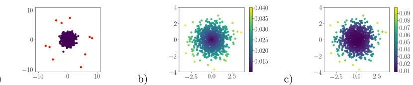
An important insight of coreset theory is that the datapoints which are different from the rest should be kept in the sample. We show in this section that one can construct a DPP which asymptotically guarantees a rebalancing of the datapoints X, meaning that points which are relatively isolated have a high chance of being retained. For instance, in the k-means setting, this property implies that, asymptotically, one can construct a DPP that provably produces a balanced sample across clusters, even in data sets where some clusters are much smaller than others. The result is illustrated in Figs. 1 and 2.

In a nutshell, the result is as follows. Suppose that the data X is a set of n elements drawn iid from a continuous distributionµdefined on Ω⊂_Rd_{. Build a projective DPPS of} sizem based on the monomials of thexi’s (see Section 3.3.1 for a precise definition). Under mild regularity assumptions on µ, we show that the intensity measure of S, marginalized over X is independent of µ. Our proof is based on a powerful theorem from Kroo and Lubinsky (2013).

Note that this rebalancing property also occurs for iid sampling with sensitivities (that provide a sort of density estimation: the lower the density of points around xi, the larger σi, the higher the chance of sampling it). What is noteworthy here is that the rebalancing property occurs “naturally”: without any sort of prior density-like estimation. We will emphasize this important point at the end of this Section.

−1.5 −1.0 −0.5 0.0 0.5 1.0 1.5

−1

0

1

x1

x2

(a)

1 2

−1.0 −0.5 0.0 0.5 1.0 −1.0 −0.5 0.0 0.5 1.0 −1.0

−0.5 0.0 0.5 1.0

x1

x2

(b)

1 2

−1.0 −0.5 0.0 0.5 1.0 −1.0 −0.5 0.0 0.5 1.0 −1.0

−0.5 0.0 0.5 1.0

x1

x2

3.3.1. Projective polynomial DPPs

The L-ensemble we shall build is based on the firstm monomials. In dimension one this

is easy to define, so we start there and generalize later to dimension d≥2. Ford= 1, we denote by X = {x1, . . . , xn} the original set (supposed to be drawn iid from µ defined on Ω), and form the n×m Vandermonde matrix

V(X) = [xj−_i 1]n,m_i,j=1 ∈_Rn×m. (16) Note that this matrix has rank m a.s. (asµ is supposed regular enough) and contains all monomials up to degree m−1. The L-ensemble we consider equals:

L=VV>∈Rn×n. (17)

The orthogonal polynomials (defined on Ω) under the empirical measuredµn= (1/n)

P

δxi

associated to X, are defined in the usual manner, i.e. q0(x) of degree 0, q1(x) of degree

1, . . . such that: R qi(x)qj(x)dµn = δij and

R

xiqj(x)dµn = 0 if i < j. In other words, the sequence is constructed from Gram-Schmidt orthogonalisation underdµn. Let us write

qj(X) = (qj(x1), . . . , qj(xn))> ∈Rn the vector consisting of the polynomial qj(x) taken at values inX. It is well-known (and easily verified) that the QR decomposition ofVverifies:

V=QR (18)

withQ= (q0(X)|. . .|qm−1(X))∈Rn×m and R∈Rm×m an upper triangular matrix.

Now, consider the m-DPPS withL-ensembleL=VV>. Using the fact that det(AB) = det(A) det(B) if Aand B are square, we have:

P(S) =Z−1det(LS)

=Z−1det((QRR>Q>)S) =Z−1det((QQ>)S) det(R)2 =Z0−1det((QQ>)S)

such thatS is also am-DPP withL-ensembleQQ>. AsQ>Q=Im,i.e.,QQ> is projective,

S is in fact a projective DPP. As a result, its associated marginal kernel is also QQ> (see Lemma. 7) and, for instance:

P(xi ∈ S) = m−1

X

j=0

q_j2(xi).

The extension tod >1 is mostly straightforward, but there are a few differences to keep in mind when defining the Vandermonde matrix of monomials. Monomialsxαare now defined as:

xα=

d

Y

j=1

x(j)αj

The total degree of a monomial equals the sum of the degrees in each variable, i.e. P

αi=

case is that there is more than one monomial of total degree φ. For example, in dimension 2,x= (x(1), x(2))>and the monomials of degree 2 are given by the powers (2,0), (0,2) and (1,1): x(1)2,x(2)2,x(1)x(2). A good way of thinking about the construction of a polynomial DPP in the multidimensional case is to pick first a maximum order (e.g. φ= 3), meaning that all monomials with total degree up to 3 are included. Then the natural sample size m for the DPP equals the total number of features, giving m = d+_φφ. Again, for d = 2 and φ= 3, this gives m = 1 + 2 + 3 + 4 = 10. In fact, there is one monomial of order 0: 1, two monomials of order 1: x(1) andx(2), three monomials of order 2 (the ones stated above), and four monomials of order 3: x(1)3,x(2)3,x(1)2x(2) and x(1)x(2)2. This implies that in dimensiond, them-DPP detailed earlier is well-defined only for specific values ofm: m= d+1₁ =d+ 1, or m= d+2₂ = ₂1(d+ 1)(d+ 2), orm= d+3₃ = 1₆(d+ 1)(d+ 2)(d+ 3), etc.

A slight technical difficulty arises in defining the orthogonal polynomials of a multivariate measure: in dimension 1, the fact that there is a single monomial of a given degree leads to a natural order in which to perform the Gram-Schmidt procedure. In higher dimensions the order is only a partial order, so that we can introduce the monomials by blocks of equal degree, but within a block the ordering is arbitrary. So we may pick any arbitrary order (e.g. lexicographic) and run Gram-Schmidt in that order (for more, see Dunkl and Xu, 2014). Given this choice the QR decomposition remains well-defined and all properties given above in the 1D case carry over to the general case. In particular, the link with the orthogonal polynomials on the discrete measure µnstays valid.

3.3.2. The rebalancing theorem

Formally, the result is as follows. The intensity function ι(x) of a point process quantifies the expected number of points to be found around x. We characterize the asymptotics of the intensity function of a DPPS when both S and the ground setX are large, and show that, in that limit, the intensity isindependent of the measure µfrom which X is sampled from.

The result is stated formally as a double limit, letting firstngo to infinity (an easy discrete-to-continuous limit), and then increasing the orderφof the polynomial DPP, which implies m going to infinity too. We emphasize that, empirically speaking, rebalancing occurs for reasonable values ofn and mbut the rate of convergence is hard to quantify.

Certain regularity assumptions are inherited from the work of Kroo and Lubinsky (2013), to which we refer for more thorough details. The formal assumptions are as follows:

1. The initial data setX ={x1, . . . , xn}is drawn i.i.d. from a measureµover a compact, convex4 domain Ω⊂_Rd_.

2. µ and the Lebesgue measure ν are mutually absolutely continuous on Ω, so thatµ0, the density, is well-defined everywhere on the domain (we use the Lebesgue measure for simplicity, another measure may be substituted)

3. We are interested in convergence “in the bulk”, ie. inside the domain. Formally, the results hold forD⊂D1⊂Ω, whereDis compact and D1 is open

4. µ0 is bounded above and below on D1

5. We form a m-DPP S on the set X, with a polynomial kernel of degree φ(defined in the previous Section), such that m= φ+_φd.

6. (technical) µis regular in the sense of Stahl, Totik, and Ullman, and the Christoffel function with respect toµ verifies condition (1.7) in Kroo and Lubinsky (2013).

The intensity measure of S, marginalizing over X, which we denote by In,φ(A) equals the expected number of points ofS in setA, i.e.:

In,φ(A) =EX,S(|S ∩ A|) =EX,S

( X

s∈S

I(s∈ A)

)

(19)

Note that the expectation is over both X and S. Furthermore, In,φ(Ω) equals m, the total number of points in S.

Our result may be stated as follows.

Theorem 16 Under the assumptions above, for all A ⊂D1,

lim φ→∞

1 φ+d

φ

_n→∞lim In,φ(A) = Z

A

κ(y)dy

where κ is a density independent of µ

The proof is in Appendix C.

Lemma 17 κ is mostly dependent on the distance to the boundaries ofΩ. For example, if

Ω is the unit ball in Rd, κ(y) =

1− ||y||2−1/2

See Kroo and Lubinsky (2013) for a proof. Several important remarks are in order:

• unlike iid sampling with sensitivities or other density-related measure for which such rebalancing property will also occur, there is here no prior density estimation: the L-ensemble is defined via the Vandermonde matrix that is trivial to compute. Thus, this rebalancing is a property that “naturally” arises from the DPP.

• this is only an asymptotic result as n and m go to infinity. Finding minimal values ofm for which rebalancing is highly probable, or even rates of convergence is likely a difficult endeavour. We emphasize nevertheless that, empirically speaking, rebalancing occurs for reasonable values ofnand m, as visible in Figs. 1 and 2.

4. Application to two problems: k-means and linear regression

We focus on two problems: k-means and linear regression. Admittedly, these are not the best problems to exhibit the usefulness of coresets: there already exists very efficient algorithms to solve them and the need for a small controlled summary is in fact rare. We nevertheless focus on these two problems as they have been well studied in the iid setting, which it is our goal to improve on. Moreover, we derived analytical formulas for the sensitivity in the 1-means and the linear regression settings: we will thus be able to compare, in those two cases, DPP sampling vs the ideal iid setting (later in the experimental Section 6).

4.1. Application to k-means

The theoretical results of Section 3 are valid for any learning problem of the form detailed in Section 2.1. We now specifically consider thek-means problem on a set X comprised of n datapoints inRd. This problem boils down to finding k centroids θ= (c1, . . . , ck), all in

Rd, such that the following cost is minimized:

L(X, θ) =X

x∈X

f(x, θ) with f(x, θ) = min

c∈θ kx−ck

2

.

Let ρ be the diameter of the minimum enclosing ball of X (the smallest ball enclosing all points in X). Theorem 8 and its corollaries are applicable to the k-means problem, such that:

Corollary 18 (m-DPP for k-means) LetSbe a sample from anm-DPP withL-ensemble L. Let , δ∈(0,1)2. With probability at least 1−δ, S is a -coreset provided that:

m≥m∗= 32

2 max i σi ¯ πi 2 kdlog 24ρ2 hfi_opt + 1

+ log4 δ

,

with ∀i,¯πi=πi/m.

Setting the marginal probabilities to their optimal values πi =mσi/S, S is a -coreset

with probability larger than 1−δ provided that:

m≥ 32

2S 2 kdlog 24ρ2 hfi_opt + 1

+ log4 δ

.

Proof Let us write B the minimum enclosing ball of X, of diameter ρ. The potentially interesting centroids are necessarily included in B such that the space of parameters Θ in the k-means setting is the set of all possiblek centroids inB: Θ =Bk_{. The metric d}

Θ we

consider is the Hausdorff metric associated with the Euclidean distance:

∀θ, θ0, dΘ(θ, θ0) = max

max c∈θ cmin0_∈θ0

c−c0

2, max_c0_∈θ0min_c∈θ

c−c0

2

.

An 0-net of Θ. Consider ΓB an 0-net of B consisting of (2ρ0 + 1)d small balls of radius

0. Such a covering indeed exists: see,e.g., Lemma 2.5 in Geer (2000). Consider Γ = Γk_B of cardinality |Γ|= (2ρ0 + 1)kd. Let us show that Γ is an0-net of Θ, that is:

In fact, considerθ= (c1, . . . , ck)∈ Bk. By construction, as ΓB is an0-net ofB, we have:

∀i= 1, . . . , k ∃c∗_i ∈ΓB s.t. kci−c∗ik ≤ 0

.

Writingθ∗ = (c∗₁, . . . , c∗_k)∈Γ, one has:

dΘ(θ, θ∗)≤0,

which proves that Γ is an 0-net of Θ. The number of balls of radius 0 =hfiopt/6γ

suffi-cient to cover Θ is thus η= (_hf12_iργ

opt + 1) kd_.

f(x, θ) isγ-Lipschitz with γ = 2ρ. Consider anyθ,θ0 andx∈ X. We want to show that:

−γ dΘ(θ, θ0)≤f(x,θ)−f(x, θ0)≤γ dΘ(θ, θ0).

Let us writec= argmint∈θkx−tk2the centroid inθclosest toxandc0 = argmint0_∈θ0kx−t0k2

the centroid inθ0 closest to x. Moreover, let us write ˜c0 = argmin_t0_∈θ0kc−t0k2 the centroid

inθ0 closest to c. Note thatc0 and ˜c0 are not necessarily equal. By definition ofc0, one has:

x−c0

≤

x−˜c0

,

such that:

x−c0

2− kx−ck2 ≤

x−˜c0

2− kx−ck2 ≤

˜c0−c

2 ≤dΘ(θ, θ

0 ).

Thus:

f(x, θ0)−f(x, θ) =x−c0(x)

2

− kx−ck2 = (x−c0

− kx−ck)( x−c0

+kx−ck)

≤(x−c0

+kx−ck) d_Θ(θ, θ0)≤2ρ d_Θ(θ, θ0).

Finally, nσmin ≥1, as shown by the second lemma of Appendix D.

Given all these elements, Theorem 8 and its subsequent corollaries are thus applicable to thek-means setting and one obtains the desired result.

Note that, in the case of DPPs, one could apply Theorem 20 to the k-means problem, and obtain similar results.

4.2. Application to linear regression

We now consider the linear regression problem: find θ ∈ _Rd _{such that a measured vector} y ∈ Rn is closest to Xθ where X> = (x1|. . .|xn) ∈ Rd×n are n data points in Rd. Let us

write Xi = (yi, xi) and X ={X1, . . . , Xn}. The least squares estimator minimizes: L(X, θ) =ky−Xθk2₂.

By denoting

one can thus write the least squares solution to the linear regression problem in the form of the problems investigated in this paper: the objective is to minimize the costL withf a positive function:

L(X, θ) =ky−Xθk2₂ = n

X

i=1

f(Xi, θ).

We suppose that all xi are enclosed in the unit ball in dimensiondand that yi∈[0,1]. Moreover, we suppose that the space Θ is bounded and enclosed in a d-dimensional ball B

centered in 0 of diameter ρ.

Even though we derived the analytical formulation of the sensitivity for linear regression (Lemma 25), we were not able to show thatnσmin≥1 in general. We thus have the following

slightly more complicated result:

Corollary 19 (m-DPP for linear regression) Let S be a sample from an m-DPP with

L-ensemble L. Let , δ ∈ (0,1)2. With probability at least 1−δ, S is a -coreset provided that:

m≥max(m∗₁, m∗₂)

with

m∗₁= 32 2 max i σi ¯ πi 2 dlog

12ρ(4ρ+ 2) hfiopt

+ 1

+ log4 δ

,

m∗₂= 32 2

1 n¯πmin

2

dlog

12ρ(4ρ+ 2) hfi_opt + 1

+ log4 δ

with ∀i,¯πi=πi/m.

Setting the marginal probabilities to their optimal values πi =mσi/S, S is a -coreset

with probability larger than 1−δ provided that:

m≥ 32

2 max

S2, S

2

n2_σ2

min

dlog

12ρ(4ρ+ 2) hfi_opt + 1

+ log4 δ

.

Proof The metric dΘ we consider is the Euclidean distance in dimensiond.

- An 0-net of Θ. Consider ΓB an 0-net of B consisting of (2ρ0 + 1)d small balls of radius

0. Such a covering indeed exists: see,e.g., Lemma 2.5 in Geer (2000). The number of balls of radius 0=hfi_opt/6γ sufficient to cover Θ is thus η= (_hf12_iργ

opt + 1) d_.

- f(X, θ) isγ-Lipschitz with γ = 4ρ+ 2. Consider any θ,θ0,xi andyi. We want to show that:

(yi−x>i θ)2−(yi−x>i θ0)2

2

≤γ2 θ−θ0

2

In fact:

(yi−x>i θ)2−(yi−x>i θ 0

)2

2

=

θ>xix>i θ−θ 0>

xix>i θ 0₋

2yix>i (θ−θ 0

)

2

=h2θ0>xix>i + (θ−θ0)>xix>i −2yix>i

θ−θ0i2

≤h 2θ

0>

xix>i + (θ−θ 0

)>xix>i −2yix>i

θ−θ0

i2

≤h2

xix

> i θ0 + xix

> i θ−θ0

+ 2y_ikx_ik i2

θ−θ0

2

by triangular inequality and writingx_ix>_i

the 2-norm of the matrixx_ix>_i , which is equal

tokxik2 and bounded by one by hypothesis. As Θ is supposed to be enclosed in a ball of radiusρ, we further have:

(yi−x>i θ)2−(yi−x>i θ0)2

2

≤(4ρ+ 2)2θ−θ0

2

Given these elements, Theorem 8 is applicable to the linear regression setting and one obtains the desired result.

5. Implementation

5.1. The DPP’s ideal marginal kernel

Following the theoretical results, the ideal strategy (although unrealistic) to build the marginal kernel K of the ideal DPP sampling scheme would be as follows. 1/ Deal with outliers as explained in Appendix E untilσmaxis not too large. 2/ Compute allσi. 3/ Set all πi tomσi/Swithmsufficiently large as detailed in the theorems. 4/ Find all non-diagonal elements ofKin order to minimize for allθthe estimator’s variance, as derived in Eq. (12):

Var( ˆL) =X i 1 πi −1

f(xi, θ)2−

X

i6=j

K2_ij

πiπj

f(xi, θ)f(xj, θ).

while constraining K to be a valid marginal kernel,i.e.: SDP with 0K1, 5/ sample a DPP with kernel K. On our way to derive a practical algorithm with a linear complexity

inn, many obstacles stand before us: there is no known polynomial algorithm to compute

5.2. A first choice: the Gaussian kernel

In order for K to be a good candidate for coresets, it needs to verify the following two properties:

• As indicated by the theorems, the diagonal entriesKiishould increase as the associated σi increases.

• As indicated by the variance equation of Eq. (12), off-diagonal elements should be as large as possible (in absolute value) given the eigenvalue constraints. In fact, we cannot set all non-diagonal entries ofK to large values as the matrix’s 2-norm would rapidly be larger than 1. We thus need to choose the best pairs (i, j) for which it is worth setting a large value of Kij. A first glance at the variance equation indicates that the larger f(xi, θ)f(xj, θ) is, the larger Kij should be, in order to decrease the variance as much as possible. Recall nevertheless that in the coreset setting, all sampling parameters should be independent of θ. The off-diagonal elements should thus verify the following property: the larger is the correlation betweenxiandxj (the more similar aref(xi, θ) and f(xj, θ) for all θ), the largerKij should be.

We show in the following in what ways the choice of marginal kernel

K=L(I+L)−1 withL the Gaussian kernel matrix with parameterτ:

∀(i, j) Lij = exp−

kx_i−x_jk2 2τ2 ,

is a good candidate to build coresets for k-means (the linear regression case is discussed later). Let us write U = (u1|. . .|un) the orthonormal eigenvector basis of L and Λ = diag(λ1|. . .|λn) its diagonal matrix of sorted eigenvalues, 0 ≤ λ1 ≤ . . . ≤ λn. U and Λ naturally depend onτ. One shows for instance that, with respect toτ,λnis a monotonically increasing function between 1 andn.

Concerning the off-diagonal elements ofK, let us first note that ifxiandxjare correlated (that is, in thek-means setting, if they are close to each other), then

Kij =

X

k λk 1 +λk

uk(i)uk(j)

should be large in absolute value. In fact, in the limit wherexi =xj, then∀k, uk(i) =uk(j) and Kij = Kii =Kjj. The determinant of the 2×2 submatrix of K indexed by i and j is therefore null: sampling both will never occur. Thus, the closer are xi and xj, the lower is the chance of sampling both jointly. Moreover, if xi and xj are far from each other (for instance, in different clusters), then the entries iand j of L0seigenvectors will be very different. For instance, say the data set contains two well separated clusters of similar size. If the Gaussian parameter τ is set to the size of these clusters, then the kernel matrix L

is necessarily small if iand j belong to different clusters, and the event of sampling both jointly is probable.

Concerning the probability of inclusion of i, we have:

Kii=

X

k λk 1 +λk

vi(k)2,

where vi is the vector of size n verifying ∀k, vi(k) = uk(i). For all i, kvik2 = 1. The probability of inclusion is thus directly linked to the values of kthat contain the energy of vi: the more the energy of vi is contained on high values ofk, the larger is the probability of inclusion. Say we are again in a situation where the clusters and the choice of Gaussian parameter τ are such that L is quasi block diagonal. Within each block, the eigenvector associated with the highest eigenvalue corresponds approximately to the constant vector. These eigenvectors being normalized, the associated entry of vi(k) is thus approximately equal to 1/√#Ci where #Ci is the size of the cluster containing data xi. Typically, if the cluster is small, that is, if #Ci tends to 1, the associated entryvi(k) tends to 1 as well, such that all the energy ofvi is drawn towards high values of k, thus increasing the probability of inclusion ofi. In other words, the more isolated, the higher the chance of being sampled. This corresponds to the intuition one may obtain for the sensitivity σi. It has indeed been shown that the sensitivity may be interpreted as a measure of outlierness (Lucic et al., 2016).

In the linear regression case, a similar argumentation is possible, up to the fact that pointican be an outlier from the point of view ofxi and/oryi, such that the kernel should take both into account: we suggest the Gaussian kernel in dimension d+ 1:

∀(i, j) Lij = exp−

kzi−zjk

2

2τ2 _,

withzi = [x>i , yi]>∈Rd+1.

In both contexts, we thus advocate to sample DPPs via a Gaussian kernel L-ensemble. We now move on to detailing an efficient sampling implementation.

5.2.1. Efficient implementation

Sampling exactly a DPP from the GaussianL-ensemble verifying

∀(i, j) Lij = exp−

kx_i−x_jk2 2τ2

consists in the following steps:

1. Compute L.

2. Diagonalize Lin its set of eigenvectors {uk}and eigenvalues {λk}.

3. Sample a DPP given {uk}and {λk}via Algorithm 1 of Kulesza and Taskar (2012).

Algorithm 1 The Gaussian kernel coreset sampling heuristics

Input: X = {xi} a set of n points in Rd, a Gaussian kernel parameter τ, a number of

samplesm

· Drawr ≥ O(m) random Fourier vectors associated to the Gaussian kernel with param-eter τ

· Compute the associated RFF matrixΨ∈_R2r×n _{as explained in Appendix F.1}

· Compute C=ΨΨ>∈_R2r×2r _{the dual representation}

· Compute the eigendecomposition of C: obtain eigenvectors {vk}and eigenvalues {νk}

· Draw a sample S from a m-DPP with L-ensemble L = Ψ>Ψ as explained in Ap-pendix F.3.

·Compute the marginal probabilitiesπsfor allxs∈ S as explained in Appendix F.3, and set weights ω(xs) = 1/πs.

Output: {S, ω} a weighted sample of sizem.

We detail in Appendix F how to reduce the overall complexity to O(nµ2), by 1/ taking advantage of Random Fourier Features (RFF) (Rahimi and Recht, 2008) to estimate a low dimensional representation Ψ∈_R2r×n _{of theL-ensembleL'Ψ}>_{Ψ, where r is the chosen} number of features; and 2/ running a DPP sampling algorithm adapted to such a low rank representation.

In the experimental section, we will concentrate on m-DPPs as they are simpler to compare with state of the art methods that all have a fixed known-in-advance number of samples. The overall m-DPP sampling algorithm adapted to the k-means problem that we will consider is summarized in Algorithm 1: given the data X, the number of desired samples m, and the Gaussian parameter τ, it outputs a weighted set of m samples S

that is a good candidate to be a coreset if m is large enough. The runtime to build Ψ is

O(ndr); to compute C and diagonalize it is O(nr2_{); to sample a m-DPP given this dual}

eigendecomposition isO(nm2). Given thatr is set to a few timesm, the overall runtime of Algorithm 1 is O(ndm+nm2).

Given a number of samples mto draw, how should one set the Gaussian parameter τ? The larger is τ, the more repulsive is them-DPP, and the smaller is the numerical rank of

Ψ(the number of eigenvaluesν such thatnν is larger than the machine’s precision). Now, numerical instabilities arise while sampling anm-DPP if the numerical rank ofΨdecreases belowm: τ should not be set too large. Also, the smaller isτ, the closer isLto the identity matrix, such that the closer is the m-DPP to uniform sampling without replacement: τ should not be set too small. We will see in the following experimental section how the choice ofτ affects results.

5.3. A second choice: a projective DPP based on the Vandermonde matrix

A second choice of DPP sampling, that derives from our analysis, is the projective DPP with m samples from the L-ensembleL =VV> where V is the Vandermonde matrix (discussed in Section 3.3.1). This choice has several advantages over the Gaussian kernel:

Algorithm 2 The Vandermonde-based coreset sampling heuristics

Input: X ={xi}a set of npoints in Rd, a number of samples m

· m should verify: ∃φ∈_N such thatm= φ+_φd. · Compute the Vandermonde matrixV∈Rn×m.

· Compute the (Q∈_Rn×m,R∈_Rm×m) decomposition ofV: V=QRwithQ>Q=Im and

Ran upper triangular matrix.

· Draw a sample S from a projective DPP with L-ensemble L = QQ> as explained in Algorithm 3.

· Compute the marginal probabilitiesπs for allxs∈ S withπs=kQ(s,:)k2 the energy of the s-th line of Q; and set weights ω(xs) = 1/πs.

Output: {S, ω} a weighted sample of sizem.

• no particular scaleτ is introduced.

This choice however has the drawback that in dimension higher than 1, not all values of m are allowed (only values of mfor which there exists φ∈Ns.t. m= φ+_φd), as explained at

the end of Section 3.3.1.

5.4. Alternative algorithms for sampling DPPs, and potential improvements

The algorithm we suggest scales in our experience rather well withn, and makes it practical to find coresets with n in the millions or more. Our method scales more poorly inm, the number of points retained, which in practice should be in the hundreds at most. Recall thatmshould scale roughly as the intrisic dimension of the parameter space: it is therefore possible that in certain difficult problems no reliable coreset can be found if5 m <1,000. With that in mind, we now review other methods for sampling DPPs.

As an alternative to direct sampling of the kind used here, MCMC methods have been suggested several times (e.g., Anari et al., 2016), and the earliest reference we could find is Belabbas and Wolfe (2009). The most basic kind starts with a set of points sampled uniformly, and uses random swapping moves: at each iteration, a point from the current set may be replaced by one not in the set.6 _{Acceptance probabilities are set so that the}

limiting distribution of the chain is the correct DPP. Each iteration has cost O(m2), and approximately O(n) such iterations are required for mixing (Hermon and Salez, 2019). The total cost is therefore the same as in our method (O(nm2)), so not much gain is to be expected here. However, there is no need for a low-rank approximation of the kernel such as the RFF approximation used here. In a nutshell, MCMC techniques sample approximately from the correct kernel instead of sampling exactly from an approximate kernel: which is better is as yet unknown but an interesting problem in itself.

There are two immediate strategies for increasingm. One is to use a crude heuristic for dividing the original data set into p different subsets, and sampling a DPP independently from each subset. This is equivalent to using a block-diagonal kernel, and along these lines there is a less radical approach, which is to force the kernel to be sparse and exploit

5. One might argue that in such cases the coreset methodology is of dubious value anyway.

sparsity in the sampling. Poulson (2019) shows how to exploit sparsity for sampling DPPs when themarginal kernel is sparse. Unfortunately, we use L-ensembles here, and one would have to adapt the tools given by Poulson to L-ensembles. A different strategy to increase m is to sample the DPP several times rather than just once. The resulting sample has less diversity but is much cheaper to generate. One can take advantage of recent methods that use pre-processing for speeding up repeated sampling of the same DPP (Gillenwater et al., 2019; Derezinski et al., 2019). Here the challenge is to find the right trade-off between computational cost and repulsion, which is again an interesting question for future research.

6. Experiments

6.1. Different strategies to compare...

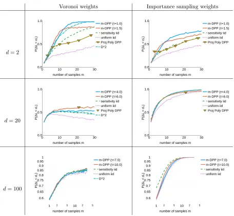
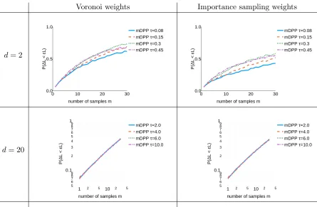
We will empirically compare results obtained with the five following approaches:

1. m-DPP: The strategy summarized in Algorithm 1.

2. PolyProj-DPP: The strategy summarized in Algorithm 2.

3. matched iid: An iid sampling strategy with replacement, matched to eitherm-DPPor PolyProj-DPP (depending on the context). More precisely,m samples are drawn iid with replacement, the probability of selectingxi at each draw being set topi=πi/m, whereπi is the marginal probability of drawing xi in m-DPP(orPolyProj-DPP).

4. uniform iid: Uniform iid sampling with replacement.

5. sensitivity iid : The current state of the art iid sampling based on a bi-criteria approximation to upper bound the sensitivity (Algorithm 2 of Bachem et al. 2017), or, if available (for instance in the case of 1-means and linear regression), an analytical formula of the sensitivity.

For the three iid methods (methods 3, 4 and 5), we will use the importance sampling esti-mator adapted to iid sampling of Eq. (6). For methods 1 and 2, we will use the importance sampling estimator adapted to correlated sampling of Eq. (8).

Empirically, when the ambient dimension d is small, performance of all methods is enhanced if the weights in ˆLare set via Voronoi cells rather than set to inverse probabilities: given the sample S of size m, compute its Voronoi tessellation in m cells, and associate to each samplexs a weightω(xs) equal to the number of datapoints in its associated Voronoi cell. We will call the associated cost estimators ˆLthe Voronoi estimators.

For completeness, we compare all these methods with another negatively correlated sampling method called D2-sampling (commonly used for k-means++ seeding, see Arthur and Vassilvitskii 2007):