Generic Inference in Latent Gaussian Process Models
Edwin V. Bonilla∗ [email protected]
Machine Learning Research Group CSIRO’s Data61
Sydney NSW 2015, Australia
Karl Krauth∗ [email protected]
Department of Electrical Engineering and Computer Science University of California
Berkeley, CA 94720-1776, USA
Amir Dezfouli [email protected]
Machine Learning Research Group CSIRO’s Data61
Sydney NSW 2015, Australia
Editor:Manfred Opper
Abstract
We develop an automated variational method for inference in models with Gaussian process (gp) priors and general likelihoods. The method supports multiple outputs and multiple latent functions and does not require detailed knowledge of the conditional likelihood, only needing its evaluation as a black-box function. Using a mixture of Gaussians as the variational distribution, we show that the evidence lower bound and its gradients can be estimated efficiently using samples fromunivariate Gaussian distributions. Furthermore, the method is scalable to large datasets which is achieved by using an augmented prior via the inducing-variable approach underpinning most sparsegp approximations, along with parallel computation and stochastic optimization. We evaluate our approach quantitatively and qualitatively with experiments on small datasets, medium-scale datasets and large datasets, showing its competitiveness under different likelihood models and sparsity levels. On the large-scale experiments involving prediction of airline delays and classification of handwritten digits, we show that our method is on par with the state-of-the-art hard-coded approaches for scalablegpregression and classification.
Keywords: Gaussian processes, black-box likelihoods, nonlinear likelihoods, scalable inference, variational inference
1. Introduction
Developing fully automated methods for inference in complex probabilistic models has be-come arguably one of the most exciting areas of research in machine learning, with notable examples in the probabilistic programming community (see e.g. Hoffman and Gelman, 2014; Wood et al., 2014; Goodman et al., 2008; Domingos et al., 2006). Indeed, while these prob-abilistic programming systems allow for the formulation of very expressive and flexible
∗. Joint first author.
c
probabilistic models, building efficient inference methods for reasoning in such systems is a significant challenge.
One particularly interesting setting is when the prior over the latent parameters of the model can be well described with a Gaussian process (gp, Rasmussen and Williams, 2006). gppriors are a popular choice in practical non-parametric Bayesian modeling with perhaps
the most straightforward and well-known application being the standard regression model with Gaussian likelihood, for which the posterior can be computed in closed form (see e.g. Rasmussen and Williams, 2006,§2.2).
Interest in gpmodels stems from their functional non-parametric Bayesian nature and
there are at least three critical benefits from adopting such a modeling approach. Firstly, by being a prior over functions, they represent a much more elegant way to address problems such as regression, where it is less natural to think of a prior over parameters such as the weights in a linear model. Secondly, by being Bayesian, they provide us with a principled way to combine our prior beliefs with the observed data in order to predict a full posterior distribution over unknown quantities, which of course is much more informative than a single point prediction. Finally, by being non-parametric, they address the common concern of parametric approaches about how well we can fit the data, since the model space is not constrained to have a parametric form.
1.1. Key Inference Challenges in Gaussian Process Models
Nevertheless, such a principled and flexible approach to machine learning comes at the cost of facing two fundamental probabilistic inference challenges, (i) scalability to large datasets and (ii) dealing with nonlinear likelihoods. With regards to the first challenge, scalability, gp models have been notorious for their poor scalability as a function of the number of training points. Despite ground-breaking work in understanding scalable gps
through the so-called sparse approximations (Qui˜nonero-Candela and Rasmussen, 2005) and in developing practical inference methods for these models (Titsias, 2009), recent literature on addressing this challenge gives a clear indication that the scalability problem is still a very active area of research, see e.g. Das et al. (2015); Deisenroth and Ng (2015); Hoang et al. (2015); Dong et al. (2017); Hensman et al. (2017); Salimbeni et al. (2018); John and Hensman (2018).
Concerning the second challenge, dealing with nonlinear likelihoods, the main difficulty is that of estimating a posterior over latent functions distributed according to a gp prior,
given observations assumed to be drawn from a possibly nonlinear conditional likelihood model. In general, this posterior is analytically intractable and one must resort to approx-imate methods. These methods can be roughly classified into stochastic approaches and deterministic approaches. The former, stochastic approaches, are based on sampling algo-rithms such as Markov Chain Monte Carlo (mcmc, see e.g. Neal, 1993, for an overview)
and the latter, deterministic approaches, are based on optimization techniques and include variational inference (vi, Jordan et al., 1998), the Laplace approximation (see e.g. MacKay,
2003, Chapter 27) and expectation propagation (ep, Minka, 2001).
On the one hand, although stochastic techniques such asmcmcprovide a flexible
con-vergence analysis. On the other hand, deterministic methods such as variational inference build upon the main insight that optimization is generally easier than integration. Conse-quently, they estimate a posterior by maximizing a lower bound of the marginal likelihood, the so-called evidence lower bound (elbo). Variational methods can be considerably faster
than mcmc but they lack mcmc’s broader applicability, usually requiring mathematical
derivations on a model-by-model basis.1 1.2. Contributions
In this paper we address the above challenges by developing a scalable automated variational method for inference in models with Gaussian process priors and general likelihoods. This method reduces the overhead of the tedious mathematical derivations traditionally inherent to variational algorithms, allowing their application to a wide range of problems. In par-ticular, we consider models with multiple latent functions, multiple outputs and non-linear likelihoods that satisfy the following properties: (i) factorization across latent functions and (ii) factorization across observations. The former assumes that, when there are more than one latent function, they are generated from independent gps. The latter assumes that,
given the latent functions, the observations are conditionally independent.
Existing gp models, such as regression (Rasmussen and Williams, 2006), binary and
multi-class classification (Nickisch and Rasmussen, 2008; Williams and Barber, 1998), warped
gps (Snelson et al., 2003), log Gaussian Cox process (Møller et al., 1998), and multi-output
regression (Wilson et al., 2012), all fall into this class of models. Furthermore, our ap-proach goes well beyond standard settings for which elaborate learning machinery has been developed, as we only require access to the likelihood function in a black-box manner. As we shall see below, our inference method can scale up to very large datasets, hence we will refer to it assavigp, which stands forscalable automated variational inference for Gaussian process models. The key characteristics of our method and contributions of this work are summarized below.
• Black-box likelihoods: As mentioned above, the main contribution of this work is to be able to carry out posterior inference withgppriors and general likelihood models,
without knowing the details of the conditional likelihood (or its gradients) and only requiring its evaluation as a black-box function.
• Scalable inference and stochastic optimization: By building upon the inducing-variable approach underpinning most sparse approximations togpmodels (Qui˜nonero-Candela
and Rasmussen, 2005; Titsias, 2009), the computational complexity of our method is dominated by O(M3) operations in time, whereM N is the number of inducing variables and N the number of observations. This is in contrast to naive inference in
gpmodels which has a time complexity of O(N3). As the resultingelbo decomposes
over the training datapoints, our model is amenable to parallel computation and stochastic optimization. In fact, we provide an implementation that can scale up to a very large number of observations, exploiting stochastic optimization, multi-core architectures and gpucomputation.
• Joint learning of model parameters: As our approach is underpinned by variational inference principles, savigp allows for learning of all model parameters, including
posterior parameters, inducing inputs, covariance hyperparameters and likelihood pa-rameters, within the same framework via maximization of the evidence lower bound (elbo).
• Multiple outputs and multiple latent functions: savigpis designed to support models
with multiple outputs and multiple latent functions, such as in multi-class classifica-tion (Williams and Barber, 1998) and non-staclassifica-tionary multi-output regression (Wilson et al., 2012). It does so in a very flexible way, allowing the differentgppriors on the
latent functions to have different covariance functions and inducing inputs.
• Flexible posterior: savigpuses a mixture of Gaussians as the approximating posterior
distribution. This is a very general approach as it is well known that, with a sufficient number of components, almost any continuous density can be approximated with arbitrary accuracy (Maz’ya and Schmidt, 1996).
• Statistical efficiency: By using knowledge of the approximate posterior and the struc-ture of thegpprior, we exploit the decomposition of theelbo, into a KL-divergence
term and an expected log likelihood term, to providestatistically efficient parameter estimates. In particular, we derive an analytical lower bound for the KL-divergence term and we show that, for general black-box likelihood models, the expected log likeli-hood term and its gradients can be computed efficiently using samples fromunivariate Gaussian distributions.
• Efficient re-parametrization: For the case of a single full Gaussian variational pos-terior, we show that it is possible to re-parametrize the model so that the optimal posterior can be represented using a parametrization that is linear in the number of observations. This parametrization becomes useful for denser models, i.e. for models that have a larger number of inducing variables.
• Extensive experimentation: We evaluatesavigpwith experiments on small datasets,
medium-scale datasets and two large datasets. The experiments on small datasets (N < 1,300) evaluate the method under different likelihood models and sparsity levels (as determined by the number of inducing variables), including problems such as regression, classification, Log Gaussian Cox processes, and warpedgps (Snelson et al.,
2003). We show that savigp can perform as well as hard-coded inference methods
under high levels of sparsity. The medium-scale experiments consider binary and multi-class classification using the mnist dataset (N = 60,000) and non-stationary
regression under the gprn model (Wilson et al., 2012) using the sarcos dataset
(N ≈45,000). Besides showing the competitiveness of our model for problems at this scale, we analyze the effect of learning the inducing inputs, i.e. the location of inducing variables. In our first large-scale experiment, we study the problem of predicting airline delays (using N = 700,000), and show that our method is on par with the state-of-the-art approach for scalable gp regression (Hensman et al., 2013), which
N = 8,100,000 observations). We show that by using this augmented dataset we can improve performance significantly. Finally, in an experiment concerning a non-linear seismic inversion problem, we show that our approach can be applied easily (without any changes to the inference algorithm) to non-standard machine learning tasks and that our inference method can match closely the solution found by more computationally demanding approaches such asmcmc.
Before describing the family of gp models that we focus on, we start by relating our
work to the previous literature concerning the key inference challenges mentioned above, i.e. scalability and dealing with non-linear likelihoods.
2. Related Work
As pointed out by Rasmussen and Williams (2006), there has been a long-standing inter-est in Gaussian processes with early work dating back at least to the 1880s when Danish astronomer and mathematician T. N. Thiel, concerned with determining the distance be-tween Copenhagen and Lund from astronomical observations, essentially proposed the first mathematical formulation of Brownian motion (see e.g. Lauritzen, 1981, for details). In geostatistics, gpregression is known as Kriging (see e.g. Cressie, 1993) where, naturally, it
has focused on 2-dimensional and 3-dimensional problems.
While the work of O’Hagan and Kingman (1978) has been quite influential in applying
gps to general regression problems, the introduction ofgp regression to main-stream
ma-chine mama-chine learning by Williams and Rasmussen (1996) sparked significant interest in the machine learning community. Indeed, henceforth, the community has takengpmodels well
beyond the standard regression setting, addressing other problems such as non-stationary and heteroscedastic regression (Paciorek and Schervish, 2004; Kersting et al., 2007; Wilson et al., 2012); nonlinear dimensionality reduction (Lawrence, 2005); classification (Williams and Barber, 1998; Nickisch and Rasmussen, 2008); multi-task learning (Bonilla et al., 2008; Yu and Chu, 2008; Alvarez and Lawrence, 2009; Wilson et al., 2012); preference learn-ing (Bonilla et al., 2010); and ordinal regression (Chu and Ghahramani, 2005). In fact, their book (Rasmussen and Williams, 2006) is the de facto reference in any work related to Gaussian process models in machine learning. As we shall see below, despite all these significant advances, most previous work in the gp community has focused on addressing
the scalability and the non-linear likelihood challenges in isolation.
2.1. Scalable Models
The cubic scaling on the number of observations of Gaussian process models, until very recently, has hindered the use of these models in a wider variety of applications. Work on approaching this problem has ranged from selecting informative (inducing) datapoints from the training data so as to facilitate sparse approximations to the posterior (Lawrence et al., 2002) to considering these inducing points as continuous parameters and optimizing them within a coherent probabilistic framework (Snelson and Ghahramani, 2006).
nonero-Candela and Rasmussen, 2005) has been extremely valuable to the community, not only to understand what those methods are actually doing but also to develop new approaches to sparse gp models. In particular, the framework of Titsias (2009) which has been placed
within a solid theoretical grounding by Matthews et al. (2016), has become the underpinning machinery of modern scalable approaches togpregression and classification. This has been
taken one step further by allowing optimization of variational parameters within a stochastic optimization framework (Hensman et al., 2013), hence enabling the applicability of these inference methods to very large datasets.
Besides variational approaches based on reverse-KL divergence minimization, other methods have adopted different inference engines, based e.g. on the minimization of the for-ward KL divergence, such as expectation propagation (Hern´andez-Lobato and Hern´ andez-Lobato, 2016). It turns out that all these methods can be seen from a more general per-spective as minimization ofα-divergences, see Bui et al. (2017) and references therein.
In addition to inducing-variable approaches to scalability ingp-models, other approaches
have exploited the relationship between infinite-feature linear-in-the-parameters models and
gps. In particular, early work investigated truncated linear-in-the-parameters models as
approximations to gpregression (see e.g. Tipping, 2001). This idea has been developed in
an alternative direction that exploits the relationship between a covariance function of a stationary process and its spectral density, hence providing random-feature approximations to the covariance function of a gp, similarly to the work of Rahimi and Recht (2008,
2009), who focused on non-probabilistic kernel machines. For example, L´azaro-Gredilla et al. (2010), Gal and Turner (2015) and Yang et al. (2015) have followed these types of approaches, with the latter mostly concerned about having fast kernel evaluations.
On another line of research, Wilson and Nickisch (2015) proposed a structured kernel interpolation method that uses local interpolation strategies that approximate the cross-covariances between the training data and the inducing inputs, while also allowing for the exploitation of Kronecker and Toeplitz algebra.
Unlike our work, none of these approaches deals with the harder task of developing scalable inference methods for multi-output problems and general likelihood models.
2.2. Multi-output and Multi-task Gaussian Processes
Developing multi-task or multi-output learning approaches using Gaussian processes has also proved an intensive area of research. Most gp-based models for these problems
Besides the work of Nguyen and Bonilla (2014b), these approaches do not scale to a very large number of observations and all of them are mainly concerned with regression problems.
2.3. General Nonlinear Likelihoods
The problem of inference in models with gp priors and nonlinear likelihoods has been
tackled from a sampling perspective with algorithms such as elliptical slice sampling (ess,
Murray et al., 2010), which are more effective at drawing samples from strongly correlated Gaussians than genericmcmcalgorithms. Nevertheless, as we shall see in Section 9.3.5, the
sampling cost of essremains a major challenge for practical usages.
From a variational inference perspective, the work by Opper and Archambeau (2009) has been slightly under-recognized by the community even though it proposes an efficient full Gaussian posterior approximation for gp models with i.i.d. observations. Our work
pushes this breakthrough further by allowing multiple latent functions, multiple outputs, and more importantly, scalability to large datasets.
Another approach to deterministic approximate inference is the integrated nested Laplace approximation (inla, Rue et al., 2009). inlauses numerical integration to approximate the marginal likelihood, which makes it unsuitable for gpmodels that contain a large number
of hyperparameters.
2.4. More Recent Developments
As mentioned in §1, the scalability problem continues to attract the interest of researchers working with gp models, with recently developed distributed inference frameworks (Gal
et al., 2014; Deisenroth and Ng, 2015), and the variational inference frameworks for scal-able gpregression and classification by Hensman et al. (2013) and Hensman et al. (2015),
respectively. As with the previous work described in §2.1, these approaches have been lim-ited to classification or regression problems or specific to a particular class of likelihood models such asgp-modulated Cox processes (John and Hensman, 2018).
Contemporarily to the work of Nguyen and Bonilla (2014a), which underpins our ap-proach, Ranganath et al. (2014) developed black-box variational inference (bbvi) for
gen-eral latent variable models. Due to this gengen-erality, it under-utilizes the rich amount of information available in Gaussian process models. For example, bbvi approximates the
KL-divergence term of the evidence lower bound but this is computed analytically in our method. Additionally, for practical reasons, bbvi imposes the variational distribution to fully factorize over the latent variables, while we make no such a restriction. A clear dis-advantage of bbvi is that it does not provide a practical way of learning the covariance
hyperparameters ofgps—in fact, these are set to fixed values. In principle, these values can
be learned inbbviusing stochastic optimization, but experimentally, we have found this to
be problematic, ineffectual, and time-consuming.
Very recently, Bonilla et al. (2016) have used the random-feature approach mentioned in Section 2.1 along with linearization techniques to provide scalable methods for inference in
gpmodels with general likelihoods. Unlike our approach for estimating expectations of the
and generally do not converge to the exact expectations even in the limit of a large number of observations.
Following the recent advances in making automatic differentiation widely available and easy to use in practical systems (see e.g. Baydin et al., 2015), developments on stochastic variational inference for fairly complex probabilistic models (Rezende et al., 2014; Kingma and Welling, 2014) can be used when the likelihood can be implemented in such systems and can be expressed using the so-called re-parametrization trick (see e.g. Kingma and Welling, 2014, for details). Nevertheless, the advantage of our method over these generic approaches is twofold. Firstly, as withbbvi, in practice such a generality comes at the cost
of making assumptions about the posterior (such as factorization), which is not suitable for
gpmodels. Secondly, and more importantly, such methods are not truly black-box as they
require explicit access to the implementation of the conditional likelihood. An interesting example where one cannot apply the re-parametrization trick is given by Challis and Barber (2013), who describe a large class of functions (that include the Laplace log likelihood) that are neither differentiable or continuous but their expectation over a Gaussian posterior is smooth. A more general setting where a truly black-box approach is required concerns inversion problems (Tarantola, 2004) where latent functions are passed through domain-specific forward models followed by a known noise model (Bonilla et al., 2016; Reid et al., 2013). These forward models may be non-differentiable, given as an executable, or too complex to re-implement quickly in an automatic differentiation framework. To illustrate this case, we present results on a seismic inversion application in §9.8.
Nevertheless, we acknowledge that some of these developments mentioned above have been extended to the gp literature, where the re-parametrization trick has been used
(Krauth et al., 2017; Matthews et al., 2017; Hensman et al., 2017; Cutajar et al., 2017). These contemporary works show that it is worthwhile building more tailored methods that may require a lower number of samples to estimate the expectations in our framework.
Finally, a related area of research is that of modeling complex data with deep belief net-works based on Gaussian process mappings (Damianou and Lawrence, 2013), which have been proposed primarily as hierarchical extensions of the Gaussian process latent variable model (Lawrence, 2005). Unlike our approach, these models target the unsupervised prob-lem of discovering structure in high-dimensional data and have focused mainly on small-data applications. However, much like the recent work on “shallow”-gparchitectures, inference
in these models have also been made scalable for supervised and unsupervised learning, ex-ploiting the reparameterization trick, e.g. using random-feature expansions (Cutajar et al., 2017) or inducing-variable approximations (Salimbeni and Deisenroth, 2017).
3. Latent Gaussian Process Models
Before starting our description of the types of models we are addressing in this paper, we refer the reader to Appendix L for a summary of the notation used henceforth.
while in others they are simply nuisance parameters and we just want to integrate them out in order to make probabilistic predictions.
A sensible modeling approach to the above problem is to assume that the Q latent functions{fj}are uncorrelated a priori and that they are drawn fromQzero-mean Gaussian processes (Rasmussen and Williams, 2006):
p(fj|θj)∼ GP(0, κj(·,·;θj)) , j= 1, . . . Q, then
p(f|θ) = Q
Y
j=1
p(f·j|θj) = Q
Y
j=1
N(f·j;0,Kjxx), (1)
where f is the set of all latent function values; f·j = {fj(xn)}Nn=1 denotes the values of latent functionj;Kjxxis the covariance matrix induced by the covariance functionκj(·,·;θj) evaluated at every pair of inputs; and θ = {θj} are the parameters of the corresponding covariance functions. Along with the prior in Equation (1), we can also assume that our multi-dimensional observations{yn}are i.i.d. given the corresponding set of latent functions
{fn}:
p(y|f,φ) = N
Y
n=1
p(yn|fn·,φ), (2)
where y is the set of all output observations; yn is the nth output observation; fn· =
{fj(xn)}Qj=1 is the set of latent function values which yn depends upon; and φ are the conditional likelihood parameters. In the sequel, we will refer to the covariance parameters (θ) as the model hyperparameters.
In other words, we are interested in models for which the following criteria are satisfied:
(i) factorization of the prior over the latent functions, as specified by Equation (1), and
(ii) factorization of the conditional likelihood over the observations given the latent func-tions, as specified by Equation (2).
We refer to the models satisfying the above assumptions (when using gp priors) as
la-tent Gaussian process models (lgpms). Interestingly, a large class of problems can be well
modeled with the above assumptions. For example binary classification (Nickisch and Ras-mussen, 2008; Williams and Barber, 1998), warpedgps (Snelson et al., 2003), log Gaussian
Cox processes (Møller et al., 1998), multi-class classification (Williams and Barber, 1998), and multi-output regression (Wilson et al., 2012) all belong to this family of models.
More importantly, besides the i.i.d. assumption, there are not additional constraints on the conditional likelihood which can be any linear or nonlinear model. Furthermore, as we shall see in §4, our proposed inference algorithm only requires evaluations of this likelihood model in a black-box manner, i.e. without requiring detailed knowledge of its implementation or its gradients.
3.1. Inference Challenges
As mentioned in §1, for general lgpms, the inference problem of estimating the posterior
a new observation x?, estimating the predictive posterior distribution p(f?·|x?,D), poses two important challenges (even in the case of a single latent function Q = 1) from the computational and statistical perspectives. These challenges are (i) scalability to large datasets and (ii) dealing with nonlinear likelihoods.
We address the scalability challenge inherent togpmodels (given their cubic time
com-plexity on the number of observations) by augmenting our priors using an inducing-variable approach (see e.g. Qui˜nonero-Candela and Rasmussen, 2005) and embedding our model into a variational inference framework (Titsias, 2009). In short, inducing variables in sparsegp
models act as latent summary statistics, avoiding the computation of large inverse covari-ances. Crucially, unlike other approaches (Qui˜nonero-Candela and Rasmussen, 2005), we keep an explicit representation of these variables (and integrate them out variationally), which facilitates the decomposition of the variational objective into a sum on the individual datapoints. This allows us to devise stochastic optimization strategies and parallel imple-mentations in cloud computing services such as Amazon EC2. Such a strategy, also allows us to learn the location of the inducing variables (i.e. the inducing inputs) in conjunction with variational parameters and hyperparameters, which in general provides better performance, especially in high-dimensional problems.
To address thenonlinear likelihood challenge, which from a variational perspective boils down to estimating expectations of a nonlinear function over the approximate posterior, we follow a stochastic estimation approach, in which we develop low-variance Monte Carlo estimates of the expected log-likelihood term in the variational objective. Crucially, we will show that the expected log-likelihood term can be estimated efficiently by using only samples from univariate Gaussian distributions.
4. Scalable Inference
Here we describe our scalable inference method for the model class specified in §3. We build upon the inducing-variable formalism underlying most sparse gp approximations
(Qui˜nonero-Candela and Rasmussen, 2005; Titsias, 2009) and obtain an algorithm with time complexity O(M3), where M is the number of inducing variables per latent process. We show that, under this sparse approximation and the variational inference framework, the expected log likelihood term and its gradient can be estimated using only samples from univariate Gaussian distributions.
4.1. Augmented Prior
In order to make inference scalable we redefine our prior in terms of some auxiliary variables
{u·j}Qj=1, which we will refer to as the inducing variables. These inducing variables lie in the same space as {f·j} and are drawn from the same zero-mean gp priors. As before,
we assume factorization of the prior across the Q latent functions. Hence the resulting augmented prior is given by:
p(u) = Q
Y
j=1
N(u·j;0,Kjzz), p(f|u) = Q
Y
j=1
N(f·j; ˜µj,Kje ), where (3)
˜
e
Kj =Kjxx−AjKjzx withAj =Kjxz(Kjzz)−1, (4)
where u·j are the inducing variables for latent processj and u is the set of all the induc-ing variables. The covariance matrices above are obtained by evaluatinduc-ing the covariance functions at the corresponding inputs, i.e., Kjzz
def
= κj(Zj,Zj;θj), Kjxx def
= κj(X,X;θj), Kjxz
def
= κj(X,Zj;θj) = (Kjzx)T, where Zj are all the inducing inputs for latent process j and X is the matrix of all input locations {xn}. We note that while each of the induc-ing variables in u·j lies in the same space as the elements in f·j, each of the M inducing inputs in Zj lies in the same space as each input data point xn. Therefore, while u·j is a M-dimensional vector, Zj is a M ×D matrix where each of the rows corresponds to a
D-dimensional inducing input. We refer the reader to Appendix L for a summary of the notation and dimensionality of the above kernel matrices.
As thoroughly investigated by Qui˜nonero-Candela and Rasmussen (2005), mostgp
ap-proximations can be formulated using the augmented prior above and additional assump-tions on the training and test conditional distribuassump-tions p(f|u) and p(f?·|u), respectively. Such approaches have been traditionally referred to as sparse approximations and we will use this terminology as well. Analogously, we will refer to models with a larger number of inducing inputs as denser models.
It is important to emphasize that the joint prior p(f,u) defined in Equation (3) is an equivalent prior to that in the original model, as if we integrate out the inducing variables u from this joint prior we will obtain the priorp(f) in Equation (1) exactly. Nevertheless, as we shall see later, following a variational inference approach and having an explicit rep-resentation of the (approximate) posterior over the inducing variables will be fundamental to scaling up inference in these types of models without making the assumptions on the training or test conditionals described in Qui˜nonero-Candela and Rasmussen (2005).
Along with the joint prior defined above, we maintain the factorization assumption of the conditional likelihood given in Equation (2).
4.2. Variational Inference and the Evidence Lower Bound
Given the prior in Equation (3) and the likelihood in Equation (2), posterior inference for general (non-Gaussian) likelihoods is analytically intractable. Therefore, we resort to approximate methods such as variational inference (Jordan et al., 1998). Variational in-ference methods entail positing a tractable family of distributions and finding the member of the family that is “closest” to the true posterior in terms of their the Kullback-Leibler divergence. In our case, we are seeking to approximate the joint posterior p(f,u|y) with a variational distribution q(f,u|λ).
4.3. Approximate Posterior
Motivated by the fact that the true joint posterior is given byp(f,u|y) =p(f|u,y)p(u|y), our approximate posterior has the form:
q(f,u|λ) =p(f|u)q(u|λ), (5)
Hence, we can define our variational distribution using a mixture of Gaussians (mog):
q(u|λ) = K
X
k=1
πkqk(u|mk,Sk) = K
X
k=1
πk Q
Y
j=1
N(u·j;mkj,Skj), (6)
where λ = {πk,mkj,Skj} are the variational parameters: the mixture proportions {πk}, the posterior means {mkj} and posterior covariances {Skj} of the inducing variables cor-responding to mixture component k and latent function j. We also note that each of the mixture components qk(u|mk,Sk) is a Gaussian with mean mk and block-diagonal covari-anceSk.
An early reference for using a mixture of Gaussians (mog) within variational inference
is given by Bishop et al. (1998) in the context of Bayesian networks. Similarly, Gershman et al. (2012) have usedmogfor non-gpmodels and, unlike our approach, used a second-order
Taylor series approximation of the variational lower bound.
4.4. Variational Lower Bound
It is easy to show that minimizing the Kullback-Leibler divergence between our approximate posterior and the true posterior, KL(q(f,u|λ)kp(f,u|y)) is equivalent to maximizing the log-evidence lower bound (Lelbo), which is composed of a KL-term (Lkl) and an expected log-likelihood term (Lell). In other words:
logp(y)≥ Lelbo(λ)def=Lkl(λ) +Lell(λ), where (7)
Lkl(λ) =−KL(q(f,u|λ)kp(f,u)), and (8)
Lell(λ) =Eq(f,u|λ)[logp(y|f)], (9)
where Eq(x)[g(x)] denotes the expectation of function g(x) over distribution q(x). Here we note that Lkl is a negative KL divergence between the joint approximate posterior
q(f,u|λ) and the joint prior p(f,u). Therefore, maximization of the Lelbo in Equation (7) entails minimization of an expected loss (given by the negative expected log-likelihoodLell) regularized by Lkl, which imposes the constraint of finding solutions to our approximate posterior that are close to the prior in the KL-sense.
An interesting observation of the decomposition of the Lelbo objective is that, unlike
Lell,Lkl in Equation (8) does not depend on the conditional likelihoodp(y|f), for which we do not assume any specific parametric form (i.e. black-box likelihood). We can thus address the technical difficulties regarding each component and their gradients separately using different approaches. In particular, for Lkl we will exploit the structure of the variational posterior in order to avoid computing KL-divergences over distributions involving all the data. Furthermore, we will obtain a lower bound forLkl in the general case ofq(u) being a mixture-of-Gaussians (mog) as given in Equation (6). For the expected log-likelihood term
4.5. Computation of the KL-divergence term (Lkl)
In order to have an explicit form forLkl and its gradients, we start by expanding Equation (8):
Lkl(λ) =−KL(q(f,u|λ)kp(f,u)) =−Eq(f,u|λ)
logq(f,u|λ)
p(f,u)
, (10)
=−Ep(f|u)q(u|λ)
logq(u|λ)
p(u)
, (11)
=−KL(q(u|λ)kp(u)), (12)
where we have applied the definition of the KL-divergence in Equation (10); used the variational joint posterior q(f,u|λ) given in Equation (5) to go from Equation (10) to Equation (11); and integrated outf to obtain Equation (12). We note that the definition of the joint posterior q(f,u|λ) in Equation (5) has been crucial to transform a KL-divergence between the joint approximate posterior and the joint prior into a KL-divergence between the variational posteriorq(u|λ) and the priorp(u) over the inducing variables. In doing that, we have avoided computing a KL-divergence between distributions over theN-dimensional variables f·j. As we shall see later, this implies a reduction in time complexity from O(N3) toO(M3), whereN is the number of datapoints andM is the number of inducing variables.
We now decompose the resulting KL-divergence term in Equation (12) as follows,
Lkl(λ) =−KL(q(u|λ)kp(u)) =Lent(λ) +Lcross(λ), where:
Lent(λ) =−Eq(u|λ)[logq(u|λ)], and
Lcross(λ) =Eq(u|λ)[logp(u)], (13)
whereLent(λ) denotes the differential entropy of the approximating distributionq(u|λ) and
Lcross(λ) denotes the negative cross-entropy between the approximating distributionq(u|λ) and the priorp(u).
Computing the entropy of the variational distribution in Equation (6), which is a mixture-of-Gaussians (mog), is analytically intractable. However, a lower bound of this
entropy can be obtained using Jensen’s inequality (see e.g. Huber et al., 2008) giving:
Lent(λ)≥ −
K
X
k=1
πklog K
X
`=1
π`N(mk;m`,Sk+S`)
def
=Lbent. (14)
The negative cross-entropy in Equation (13) between a Gaussian mixture q(u|λ) and a Gaussianp(u), can be obtained analytically,
Lcross(λ) =− 1 2
K
X
k=1
πk Q
X
j=1
[Mlog 2π+ logKjzz
+mTkj(Kjzz)−1mkj + tr (Kjzz)−1Skj]. (15)
4.6. Estimation of the expected log likelihood term (Lell)
We now address the computation of the expected log likelihood term in Equation (9). The main difficulty of computing this term is that, unlike theLkl where we have full knowledge of the prior and the approximate posterior, here we do not assume a specific form for the conditional likelihoodp(y|f,φ). Furthermore, we only require evaluations of logp(yn|fn·,φ) for each datapointn, hence yielding a truly black-box likelihood method.
We will show one of our main results, that ofstatistical efficiency of ourLell estimator. This means that, despite having a full Gaussian approximate posterior, estimation of the
Lell and its gradients only requires samples from univariate Gaussian distributions. We start by expanding Equation (9) using our definitions of the approximate posterior and the factorization of the conditional likelihood:
Lell(λ) =Eq(f,u|λ)[logp(y|f,φ)] =Eq(f|λ)[logp(y|f,φ)], (16) where, given the definition of the approximate joint posteriorq(f,u|λ) in Equation (5), the distributionq(f|λ) resulting from marginalizingufrom this joint posterior can be obtained analytically,
q(f|λ) = K
X
k=1
πkqk(f|λk) = K
X
k=1
πk Q
Y
j=1
N(f·j;bkj,Σkj), with (17)
bkj =Ajmkj, and (18)
Σkj =Kje +AjSkjATj, (19)
where Kje and Aj are given in Equation (4) and, as defined before, {mkj} and {Skj} are
the posterior means and posterior covariances of the inducing variables corresponding to mixture component k and latent function j. We are now ready to state our result of a statistically efficient estimator for theLell:
Theorem 1 For the gp model with prior defined in Equations (3) to (4), and conditional likelihood defined in Equation(2), the expected log likelihood over the variational distribution in Equation(5) and its gradients can be estimated using samples from univariate Gaussian distributions.
The proof is constructive and can be found in Appendix B. We note that a less general result, for the case of one latent function and a single variational Gaussian posterior, was obtained in Opper and Archambeau (2009) using a different derivation. Here we state our final result on how to compute these estimates:
Lell(λ) = N
X
n=1 K
X
k=1
πkEqk(n)(fn·|λk)[logp(yn|fn·,φ)], (20)
∇λkLell(λ) =πk N
X
n=1
Eqk(n)(fn·|λk)
∇λklogqk(n)(fn·|λk) logp(yn|fn·,φ), forλk ∈ {mk,Sk},
∇πkLell(λ) = N
X
n=1
Eqk(n)(fn·|λk)[logp(yn|fn·,φ)], (22)
whereqk(n)(fn·|λk) is a Q-dimensional Gaussian with:
qk(n)(fn·|λk) =N(fn·;bk(n),Σk(n)),
where Σk(n) is a diagonal matrix. The jth element of the mean and the (j, j)th entry of the covariance of the above distribution are given by:
[bk(n)]j =aTjnmkj, [Σk(n)]j,j = [Kje ]n,n+aTjnSkjajn, (23)
whereaTjndef= [Aj]n,:denotes theM-dimensional vector corresponding to thenth row of ma-trixAj;Kej andAj are given in Equation (4); and, as before,{mkj,Skj}are the variational
parameters corresponding to the mean and covariance of the approximate posterior over the inducing variables for mixture component kand latent process j.
We emphasize that when Q > 1, qk(n)(fn·|λk) is not a univariate marginal but a Q -dimensional marginal posterior with diagonal covariance. Therefore, only samples from univariate Gaussians are required to estimate the expressions in Equations (20) to (22).
4.6.1. Practical consequences and unbiased estimates
There are two immediate practical consequences of the result in Theorem 1. The first consequence is that we can use unbiased empirical estimates of the expected log likelihood term and its gradients. In our experiments we use Monte Carlo (mc) estimates, hence we
can computeLell as:
n
fn·(k,i)
oS
i=1∼ N(fn·;bk(n),Σk(n)),k= 1, . . . , K,
b Lell= 1
S
N
X
n=1 K
X
k=1
πk S
X
i=1
logp(yn|fn·(k,i),φ), (24)
where bk(n) and Σk(n) are the vector and matrix forms of the mean and covariance of the posterior over the latent functions as given in Equation (23). Analogous mc estimates of
the gradients are given in Appendix C.2.
The second practical consequence is that in order to estimate the gradients of the Lell, using Equations (21) and (22), we only require evaluations of the conditional likelihood in a black-box manner, without resorting to numerical approximations or analytical derivations of its gradients.
5. Parameter Optimization
In order to learn the parameters of our model we seek to maximize our (estimated) log-evidence lower bound (Lbelbo) using gradient-based optimization. Letη ={λ,θ,φ} be all
the model parameters for which point estimates are required. We have that:
b
∇ηLbelbo=∇ηLbent+∇ηLcross+∇ηLbell,
where we have made explicit the dependency of the log-evidence lower bound on any pa-rameter of the model and Lbent, Lcross, and Lbell are given in Equations (14), (15), (24)
respectively. The gradients ofLbelbo wrt variational parameters λ, covariance
hyperparam-etersθ and likelihood parameters φare given in Appendices C, D.1, and D.2, respectively. As shown in these appendices, not all constituents of Lbelbo contribute to learning all
pa-rameters, for example∇θLbent =∇φLbent=∇φLcross = 0.
Using the above objective function (Lbelbo) and its gradients we can consider batch
opti-mization with limited-memorybfgsfor small datasets and medium-size datasets. However,
under this batch setting, the computational cost can be too large to be afforded in practice even for medium-size datasets on single-core architectures.
5.1. Stochastic optimization
To deal with the above problem, we first note that the terms corresponding to the KL-divergenceLbent and Lcross in Equations (14) and (15) do not depend on the observed data,
hence their computational complexity is independent ofN. More importantly, we note that
b
Lell in Equation (24) decomposes as a sum of expectations over individual datapoints. This makes our inference framework amenable to parallel computation and stochastic optimiza-tion (Robbins and Monro, 1951). More precisely, we can rewrite Lbelbo as:
b Lelbo=
N
X
n=1
1
N
b
Lent+Lcross
+Lb
(n) ell
,
whereLb
(n) ell =
1 S
PK
k=1πkPSi=1logp(yn|fn·(k,i),φ), which enables us to apply stochastic opti-mization techniques such as stochastic gradients descend (sgd, Robbins and Monro, 1951) or adadelta (Zeiler, 2012). The complexity of the resulting algorithm is independent of
N and dominated by algebraic operations that are O(M3) in time, where M is the num-ber of inducing points per latent process. This makes our automated variational inference framework practical for very large datasets.
5.2. Reducing the variance of the gradients with control variates
Theorem 1 is fundamental to having a statistical efficient algorithm that only requires sam-pling from univariate Gaussian distributions (instead of samsam-pling from very high-dimensional Gaussians) for the estimation of the expected log likelihood term and its gradients.
However, the variance of the gradient estimates may be too large for the algorithm to work in practice, and variance reduction techniques become necessary. Here we use the well-known technique of control variates (see e.g. Ross, 2006,§8.2), where a new gradient estimate is constructed so as to have the same expectation but lower variance than the original estimate. Our control variate is the so-called score function h(fn·) = ∇λklogqk(n)(fn·|λk)
5.3. Optimization of the inducing inputs
So far we have discussed optimization of variational parameters (λ), i.e. the parameters of the approximate posterior ({πk,mk,Sk}); covariance hyperparameters (θ); and likelihood parameters (φ). However, as discussed by Titsias (2009), the inducing inputs {Zj} can be seen as additional variational parameters and, therefore, their optimization should be somehow robust to overfitting. As described in the Experiments (Section 9.5), learning of the inducing inputs can improve performance, requiring a lower number of inducing variables than when these are fixed. This, of course, comes at an additional computational cost which can be significant when considering high-dimensional input spaces. As with the variational parameters, we study learning of the inducing inputs via gradient-based optimization, for which we use the gradients provided in Appendix E.
Early references in the machine learning community where a single variational objective is used for parameter inference (in addition to posterior estimation over latent variables) can be found in Hinton and van Camp (1993); MacKay (1995); Lappalainen and Miskin (2000). These methods are now known under the umbrella term of variational Bayes2 and consider a prior and an approximate posterior for these parameters within the variational framework. As mentioned above, rather than a full variational Bayes approach, we provide point estimates of {θ,φ} and {Zj}, and our experiments in §9 confirm the efficacy of our approach. More specifically, we show in §9.5 that point-estimation of the inducing inputs
{Zj} using the variational objective can be significantly better than using heuristics such as k-means clustering.
6. Dense Posterior and Practical Distributions
In this section we consider the case when the inducing inputs are placed at the training points, i.e. Zj = X and consequently M = N. As mentioned in Section 4.1, we refer to this setting as dense to distinguish it from the case whenM < N, for which the resulting models are usually called sparse approximations. It is important to realize that not all real datasets are very large and that in many cases the resulting time and memory complexity
O(N3) and O(N2) can be afforded. Besides the dense posterior case, we also study some particular variational distributions that make our framework more practical, especially in large-scale applications.
6.1. Dense Approximate Posterior
When our posterior is dense the only approximation made is the assumed variational dis-tribution in Equation (6). We will show that, in this case, we recover the objective function in Nguyen and Bonilla (2014a) and that hyper-parameter learning is easier as the terms in the resulting objective function that depend on the hyperparameters do not involve mc
estimates. Therefore, their analytical gradients can be used. Furthermore, in the following
section, we will provide an efficient exact parametrization of the posterior covariance that reduces the O(N2) memory complexity to a linear complexity O(N).
We start by looking at the components of Lelbo when we make Zj = X, which we can simply obtain by making Kjzz = Kjxx and M = N, and realizing that the posterior
parameters {mkj,Skj} are now N-dimensional objects. Therefore, we leave the entropy termLbent in Equation (14) unchanged and we replace all the appearances ofK
j
zzwithKjxx
and all the appearances ofM withN for theLcross. We refer the reader to Appendix G for details of the equations but it is easy to see that the resulting Lbent and Lcross are identical to those obtained by Nguyen and Bonilla (2014a, Equations 5 and 6).
For the expected log likelihood term, the generic expression in Equation (16) still applies but we need to figure out the resulting expressions for the approximate posterior parame-ters in Equations (18) and (19). It is easy to show that the resulting posterior means and covariances are in factbkj =mkj andΣkj =Skj (see Appendix G for details). This means that in the dense case we simply estimate theLbell by using empirical expectations over the
unconstrained variational posterior q(f|λ), with ‘free’ mean and covariance parameters. In contrast, in the sparse case, although these expectations are still computed overq(f|λ), the parameters of the variational posterior q(f|λ) are constrained by Equations (18) and (19) which are functions of the prior covariance and the parameters of the variational distribution over the inducing variables q(u|λ). As we shall see in the following section, this distinc-tion between the dense case and sparse case has critical consequences on hyperparameter learning.
6.1.1. Exact Hyperparameter Optimization
The above insight reveals a remarkable property of the model in the dense case. Unlike the sparse case, the expected log likelihood term does not depend on the covariance hyper-parameters, as the expectation of the conditional likelihood is taken over the variational distribution q(f|λ) with ‘free’ parameters. Therefore, only the cross-entropy term Lcross
depends on the hyperparameters (as we also know that∇θLbent = 0). For this term, as seen
in Appendix G.1 and corresponding gradients in Equation (37), we have derived the exact (analytical) expressions for the objective function and its gradients, avoiding empiricalmc
estimates altogether. This has a significant practical implication: despite using black-box inference, the hyperparameters are optimized wrt the true evidence lower bound (given fixed variational parameters). This is an additional and crucial advantage of our automated inference method over other generic inference techniques (see e.g. Ranganath et al., 2014), which do not exploit knowledge of the prior.
6.1.2. Exact Solution with Gaussian Likelihoods
Another interesting property of our approach arises from the fact that, as we are usingmc
estimates,Lbellis an unbiased estimator of Lell. This means that, as the number of samples
S increases,Lbelbo will converge to the true valueLelbo. In the case of a Gaussian likelihood,
6.2. Practical Variational Distributions
As we have seen in Section 5, learning of all parameters in the model can be done in a scalable way through stochastic optimization for general likelihood models, providing au-tomated variational inference for models with Gaussian process priors. However, the gen-eral mog approximate posterior in Equation (6) requiresO(M2) variational parameters for
each covariance matrix of the corresponding latent process, yielding a total requirement of
O(QKM2) parameters. This may cause difficulties for learning when these parameters are optimized simultaneously. In this section we introduce two special members of the assumed variational posterior family that improve the practical tractability of our inference frame-work. These members are a full Gaussian posterior and a mixture of diagonal Gaussians posterior.
6.2.1. Full Gaussian Posterior
This instance considers the case of only one component in the mixture (K = 1) in Equation (6),which has a Gaussian distribution with afull covariance matrix for each latent process. Therefore, following the factorization assumption in the posterior across latent processes, the posterior distribution over the inducing variables u, and consequently over the latent functionsf, is a Gaussian with block diagonal covariance, where each block is a full covari-ance corresponding to that of a single latent function. We thus refer to this approximate posterior as the full Gaussian posterior (fg).
6.2.2. Mixture of Diagonal Gaussians Posterior
Our second practical variational posterior considers a mixture distribution as in Equation (6), constraining each of the mixture components for each latent process to be a Gaus-sian distribution with diagonal covariance matrix. Therefore, following the factorization assumption in the posterior across latent processes, the posterior distribution over the in-ducing variables u is a mixture of diagonal Gaussians. However, we note that, as seen in Equations (18) and (19), the posterior over the latent functions f is not a mixture of diagonal Gaussians in the general sparse case. Obviously, in the dense case (whereZj =X) the posterior covariance over f of each component does have a diagonal structure. Hence-forth, we will refer to this approximation simply asmog, to distinguish it from the fgcase
above, while avoiding the use of additional notation. One immediate benefit of using this approximate posterior is computational, as we avoid the inversion of a full covariance for each component in the mixture.
As we shall see in the following sections, there are additional benefits from the assumed practical distributions and they concern the efficient parametrization of the covariance for both distributions and the lower variance of the gradient estimates for themog posterior.
6.3. Efficient Re-parametrization
As mentioned above, one of the main motivations for having specific practical distribu-tions is to reduce the computational overhead due to the large number of parameters to optimize. For the mog approximation, it is obvious that only O(M) parameters for each
hence one obtains an efficient parametrization by definition. However, for the full Gaussian (fg) approximation, naively, one would require O(M2) parameters. The following theorem
states that for settings that require a large number of inducing variables, thefgvariational
distribution can be represented using a significantly lower number of parameters.
Theorem 2 The optimal full Gaussian variational posterior can be represented using a parametrization that is linear in the number of observations (N).
Before proceeding with the analysis of this theorem, we remind the reader that the general form of our variational distribution in Equation (6) requiresO(KQM2) parameters for the covariance, for a model with K mixture components, Q latent processes and M inducing variables. Nevertheless, for simplicity and because usually K M and Q M, we will omitK and Qin in the following discussion.
The proof the theorem can be found in Appendix H, where it is shown that in the fg
case the optimal solution for the posterior covariance is given by:
c
Sj =Kjzz Kjzz+KjzxΛjKjxz −1
Kjzz, (25)
whereΛjis aN-dimensional diagonal matrix. Since the optimal covariance can be expressed in terms of fixed kernel computations and a free set of parameters given by Λj, only N
parameters are necessary to represent the posterior covariance. As we shall see below, this parametrization becomes useful for denser models, i.e. for models that have a large number of inducing variables.
6.3.1. Sparse Posterior
In the sparse case the inducing inputsZj are at arbitrary locations and, more importantly,
M N, the number of inducing variables is considerably smaller than the number of training points. The result in Equation (25) implies that if we parameterizeSj in that way, we will need O(N) parameters instead of O(M2). Of course this is useful when roughly
N < M22. A natural question arises when we define the number of inducing points as a fraction of the number of training points, i.e. M = N with 0 ≤ ≤ 1, when is such a parameterization useful? In this case, using the alternative parametrization will become
beneficial when >
q
2
N. To illustrate this, consider for example the mnist dataset used in our medium-scale experiments in Section 9.4 whereN = 60,000. This yields a beneficial regime around roughly >0.006, which is a realistic setting. In fact, in our experiments on this dataset we did consider sparsity factors of this magnitude. For example, our biggest experiment used = 0.04. With a naive parametrization of the posterior covariance, we would need roughly 2×10⁶ parameters. In contrast, by using the efficient parametrization we only need 50×103 parameters. As shown below, these gains are greater as the model becomes denser, yielding a dramatic reduction in the number of parameters when having a fully dense Gaussian posterior.
6.3.2. Dense Posterior
In the dense case we have thatZj =X,∀j= 1, . . . , Qand consequentlyM =N. Therefore we have that the optimal posterior covariance is given by:
c
In principle, the parametrization of the posterior covariance would requireO(N2) parame-ters for each latent process. However, the above result shows that we can parametrize these covariances efficiently using onlyO(N) parameters.
We note that, for models with Q= 1, this efficient re-parametrization has been used by Sheth et al. (2015) in the sparse case and Opper and Archambeau (2009) in the dense case, while adopting an inference algorithm different to ours.
6.4. Automatic Variance Reduction with a Mixture-of-Diagonals Posterior
An additional benefit of having a mixture-of-diagonals (mog) posterior in the dense case is
that optimization of the variational parameters will typically converge faster when using a mixture of diagonal Gaussians. This is an immediate consequence of the following theorem.
Theorem 3 When having a dense posterior, the estimator of the gradients wrt the vari-ational parameters using the mixture of diagonal Gaussians has a lower variance than the full Gaussian posterior’s.
The proof is in Appendix I and is simply a manifestation of the Rao-Blackwellization tech-nique (Casella and Robert, 1996). The theorem is only made possible due to the analytical tractability of the KL-divergence term (Lkl) in the variational objective (Lelbo). The practi-cal consequence of this theorem is that optimization will typipracti-cally converge faster when using a mixture-of-diagonals Gaussians than when using a full Gaussian posterior approximation.
7. Predictions
Given the general posterior over the inducing variablesq(u|λ) in equation (6), the predictive distribution for a new test pointx? is given by:
p(y?|x?) = K
X
k=1
πk
Z
p(y?|f?·)
Z
p(f?·|u)qk(u|λk)dudf?·.
= K
X
k=1
πk
Z
p(y?|f?·)qk(f?·|λk)df?·, (26)
whereqk(f?·|λk) is the predictive distribution over the Qlatent functions corresponding to mixture componentk given the learned variational parametersλ={mk,Sk}:
qk(f?·|λk) = Q
Y
j=1
N(f?j;µ?kj, σ?2kj), with
µ?kj =κj(x?,Zj)(Kjzz)
−1
mkj, and
σ?2kj =κj(x?,x?)−κj(x?,Zj) (Kjzz)
−1−
(Kjzz)−1Skj(Kjzz)
−1
κj(Zj,x?).
8. Complexity analysis
Throughout this paper we have only considered computational complexity with respect to the number of inducing points and training points for simplicity. Although this has also been common practice in previous work (see e.g. Dezfouli and Bonilla, 2015; Nguyen and Bonilla, 2014a; Hensman et al., 2013; Titsias, 2009), we believe it is necessary to provide an in-depth complexity analysis of the computational cost of our model. Here we analyze the computational cost of evaluating the Lelbo and its gradients once.
We begin by reminding the reader of the dimensionality notation used so far and by introducing additional notation specific to this section. We analyze the more general case of stochastic optimization using mini-batches. Let K be the number of mixture components in our variational posterior;Qthe number of latent functions; Dthe dimensionality of the input data;S the number of samples used to estimate the required expectations via Monte Carlo;B the number of inputs used per mini-batch; M the number of inducing inputs; and
N the number of observations. We note that in the case of batch optimizationB =N, hence our analysis applies to both the stochastic and batch setting. We also let T(e) represent the computational costs of expressione. Furthermore, we assume that the kernel function is simple enough such that evaluating its output between two points isO(D) and we denote withT(logp(yn|fn·,φ))∈ O(L) the cost of a single evaluation of the conditional likelihood.
8.1. Overall Complexity
While the detailed derivations of the computational complexity are in Appendix J, here we state the main results. Assuming thatK M, the total computational cost is given by:
T(Lelbo)∈ O(Q(M2D+BM D+K2M3+KBM2+KBSL)), and for diagonal posterior covariances we have:
T(Lelbo)∈ O(Q(M2D+BM D+M3+KBM +KBSL)).
We note that it takes dN/Be gradient updates to go over an entire pass of the data. If we assume thatK is a small constant, the asymptotic complexity of a single pass over the data does not improve by increasingB beyond B=M. Hence if we assume thatB ∈ O(M) the computational cost of a single gradient update is given by
T(Lelbo)∈ O(QM(M D+M2+SL)),
for both diagonal and full covariances. If we assume that it takes a constant amount of time to compute the likelihood function between a sample and an output, we see that setting
S ∈ O(M D+M2) does not increase the computational complexity of our algorithm. As we shall see in section 9.4, even a complex likelihood function only requires 10,000 samples to approximate it. Since we expect to have more than 100 inducing points in most large scale settings, it is reasonable to assume that the overhead from generated samples will not be significant in most cases.
9. Experiments
performance of the model when considering different likelihoods and different dataset sizes. We analyze how our algorithm’s performance is affected by the density and location of the inducing variables, and how the performance of batch and stochastic optimization compare. We start by evaluating our algorithm using five small-scale datasets (N <1,300) under different likelihood models and number of inducing variables (§9.3). Then, using medium-scale experiments (N < 70,000), we compare stochastic and batch optimization settings, and determine the effect of learning the inducing inputs on the performance (§9.4). Sub-sequently, we usesavigp on two large-scale datasets. The first one involves the prediction
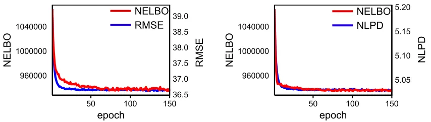
of airline delays, where we compare the convergence properties of our algorithm to models that leverage full knowledge of the likelihood (§9.7.1). The second large dataset considers an augmented version of the popular mnist dataset for handwritten digit recognition,
in-volving more than 8 million observations (§9.7.3). Finally, we showcase our algorithm on a non-standard inference problem concerning a seismic inversion task, where we show that our variational inference algorithm can yield solutions that closely match (non-scalable) sam-pling approaches (§9.8). Before proceeding with the experimental set-up, we give details of our implementation which uses gpus.
9.1. Implementation
We have implemented our savigpmethod in Python and all the code is publicly available
at https://github.com/Karl-Krauth/Sparse-GP. Most current mainstream implemen-tations of Gaussian process models do not support gpu computation, and instead opt to
offload most of the work to thecpu, with the notable exception of Matthews et al. (2017).
For example, neither of the popular packages gpml3 or gpy4 provide support for gpus.
This is despite the fact that matrix manipulation operations, which are easily paralleliz-able, are at the core of any Gaussian process model. In fact, the rate of progress between subsequent gpu models has been much larger than for cpus, thus ensuring that any gpu
implementation would run at an accelerated rate as faster hardware gets released.
With these advantages in mind, we provide an implementation of savigp that uses Theano (Al-Rfou et al., 2016), a library that allows users to define symbolic mathematical expressions that get compiled to highly optimized gpu cuda code. Any operation that
involved the manipulation of large matrices or vectors was done in Theano. Most of our experiments were either run on g2.2 awsinstances, or on a desktop machine with an Intel
core i5-4460 cpu, 8GB of ram, and agtx760 gpu.
Despite using a low-end outdated gpu, we found a time speed-up of 5x on average when
we offloaded work to the gpu. For example, in the case of the mnist-b dataset (used in
section 9.4), we averaged the time it took to compute ten gradient evaluations of theLelbo with respect to the posterior parameters over the entire training set, where we expressed the posterior as a full Gaussian and used a sparsity factor of 0.04. While it took 42.35 seconds, on average, per gradient computation when making use of the cpu only, it took
a mere 8.52 seconds when work was offloaded to the gpu. We expect the difference to be
even greater given a high-end current-generationgpu.
9.2. Details of the Experiments
Here we give details of our experimental evaluation concerning performance measures, in-ducing input learning, optimization methods, how to read the figures reported and the different model configurations explored.
9.2.1. Performance Measures
We evaluated the performance of the algorithm using non-probabilistic and probabilistic measures according to the type of learning problem we are addressing. The standardized squared error (sse) and the negative log predictive density (nlpd) were used in the case
of continuous-output problems. The error rate (er) and the negative log probability (nlp)
were used in the case of discrete-output problems. In the experiments using the airline dataset, we used the root mean squared error (rmse) instead of the sse to be able to
compare our method with previous work that usedrmse for performance evaluation.
9.2.2. Experimental Settings
In small-scale experiments, inducing inputs were placed on a subset of the training data in a nested fashion, so that experiments on less sparse models contained the inducing points of the sparser models. In medium-scale and large-scale experiments the location of the inducing points was initialized using thek-means clustering method. In all experiments the squared exponential covariance function was used.
9.2.3. Optimization Methods
Learning the model involves optimizing variational parameters, hyperparameters, likelihood parameters, and inducing inputs. These were optimized iteratively in a global loop. In every iteration, each set of parameters was optimized separately while keeping the other sets of parameters fixed, and this process was continued until the change in the objective function between two successive iterations was less than 10−6. For optimization in the batch settings, each set of parameters was optimized using l-bfgs, with the maximum number of global
iterations limited to 200. In the case of stochastic optimization, we used the adadelta
method (Zeiler, 2012) with parameters= 10−6and a decay rate of 0.95. The choice of this optimization algorithm was motivated by (and to be consistent with) the work of Hensman et al. (2013), who found this specific algorithm successful in the context of Gaussian process regression. We compare with the method of Hensman et al. (2013) in this context in §9.7.
9.2.4. Reading the Graphs
Dataset Ntrain Ntest D Likelihoodp(y|f) Model
mining 811 0 1 λyexp(−λ)/y! Log Gaussian Cox process boston 300 206 13 N(y;f, σ2) Standard regression
creep 800 1266 30 ∇yt(y)N(t(y);f, σ2) Warped Gaussian processes abalone 1000 3177 8 ∇yt(y)N(t(y);f, σ2) Warped Gaussian processes
cancer 300 383 9 1/(1 + exp(−f)) Binary classification usps 1233 1232 256 exp(fc)/Pi=1exp(fi) Multi-class classification
Table 1: Details of the datasets used in the small-scale experiments and their corresponding likelihood models. Ntrain, Ntest, D are the number of training points, test points and input dimensions respectively; ‘likelihood’ is the conditional likelihood used on each problem; and ‘model’ is the name of the model associated with that likelihood. ForminingNtest= 0 as only posterior inference is done (predictions on a test set are not made for this problem).
9.2.5. Model Configurations
We refer to the ratio of inducing points to training points as the sparsity factor (SF =M/N). For each sparsity factor, three different variations of savigp corresponding to (i) a full
Gaussian posterior, (ii) a diagonal Gaussian posterior, and (iii) a mixture of two diagonal Gaussian posteriors were tested, which are denoted respectively byfg,mog1, andmog2in
the graphs.
9.3. Small-scale Experiments
We testedsavigpon six small-scale datasets with different likelihood models. The datasets
are summarized in Table 9.3, and are the same as those used by Nguyen and Bonilla (2014a). For each dataset, the model was tested five times across different subsets of the data; except for the mining dataset where only training data were used for evaluation of the posterior distribution.
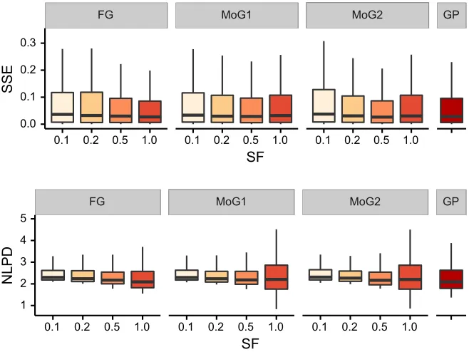
9.3.1. Standard Regression
The model was evaluated on thebostondataset (Bache and Lichman, 2013), which involves
a standard regression problem with a univariate Gaussian likelihood model, i.e.,p(yn|fn) =
N(yn|fn, σ2). Figure 1 shows the performance of savigp for different sparsity factors, as
well as the performance of exact Gaussian process inference (gp). As we can see, sse
increases slightly on sparser models. However, thesse of all the models (fg,mog1,mog2)
across all sparsity factors are comparable to the performance of exact inference (gp). In
terms of nlpd, as expected, the dense (SF = 1) fg model performs exactly like the exact
inference method (gp). In the sparse models, nlpd shows less variation in lower sparsity
factors (especially for mog1 and mog2), which can be attributed to the tendency of such
FG MoG1 MoG2 GP
0.0 0.1 0.2 0.3
0.1 0.2 0.5 1.0 0.1 0.2 0.5 1.0 0.1 0.2 0.5 1.0 SF
SSE
FG MoG1 MoG2 GP
1 2 3 4 5
0.1 0.2 0.5 1.0 0.1 0.2 0.5 1.0 0.1 0.2 0.5 1.0 SF
NLPD
Figure 1: The distributions of sse and nlpd for a regression problem with a univariate
Gaussian likelihood model on the boston housing dataset. Three approximate
posteriors insavigpare used: fg(full Gaussian),mog1(diagonal Gaussian), and mog2 (mixture of two diagonal Gaussians), along with various sparsity factors
(SF =M/N). The smaller thesfthe sparser the model, with SF = 1
correspond-ing to the dense model. gp corresponds to the performance of exact inference using standard Gaussian process regression.
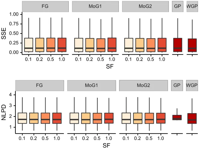
9.3.2. Warped Gaussian Process
In warped Gaussian processes, the likelihood function isp(yn|fn) =∇yt(yn)N(t(yn);fn, σ2), for some transformation t. We used the same neural-net style transformation as Snelson et al. (2003), and evaluated the performance of our model on two datasets: creep (Cole
et al., 2000), andabalone(Bache and Lichman, 2013). The results are compared with the
performance of exact inference for warped Gaussian processes (wgp) described by Snelson
et al. (2003), and also with the performance of exact Gaussian process inference with a univariate Gaussian likelihood model (gp). As shown in Figure 2, in the case of theabalone
dataset, the performance is similar across all the models (fg,mog1andmog2) and sparsity
factors, and is comparable to the performance of the exact inference method for warped Gaussian processes (wgp). The results on creepare given in Appendix K.1.
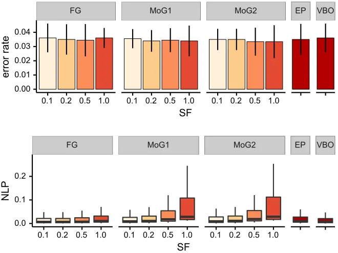
9.3.3. Binary Classification