A Spectral Algorithm for Inference in Hidden semi-Markov Models
Igor Melnyk [email protected]
IBM T. J. Watson Research Center Yorktown Heights, NY 10598, USA
Arindam Banerjee [email protected]
Department of Computer Science and Engineering University of Minnesota
Minneapolis, MN 55414, USA
Editor:Le Song
Abstract
Hidden semi-Markov models (HSMMs) are latent variable models which allow latent state persis-tence and can be viewed as a generalization of the popular hidden Markov models (HMMs). In this paper, we introduce a novel spectral algorithm to perform inference in HSMMs. Unlike expec-tation maximization (EM), our approach correctly estimates the probability of given observation sequence based on a set of training sequences. Our approach is based on estimating moments from the sample, whose number of dimensions depends only logarithmically on the maximum length of the hidden state persistence. Moreover, the algorithm requires only a few matrix inversions and is therefore computationally efficient. Empirical evaluations on synthetic and real data demonstrate the advantage of the algorithm over EM in terms of speed and accuracy, especially for large data sets.
Keywords: Graphical models, hidden semi-Markov model, spectral algorithm, tensor analysis, aviation safety
1. Introduction
Hidden semi-Markov models (HSMMs) are discrete latent variable models which allow temporal persistence of latent states, and can be viewed as a generalization of the popular hidden Markov models (HMMs) (Chiappa, 2014; Murphy, 2002; Yu, 2010). In HSMMs, the stochastic model for the unobservable process is defined by a semi-Markov chain: latent state at the next time step is determined by the current latent state as well as time elapsed since the entry into the current state. The ability to flexibly model such latent state persistence turns out to be useful in many application areas, including anomaly detection (Tan and Xi, 2008; Xie and Yu, 2009), activity recognition (van Kasteren et al., 2010), and speech synthesis (Zen et al., 2007). Such state persistence is in contrast to HMMs, which use a Markov chain over latent state transitions and hence have an implicit geometric distribution for the state duration (Rabiner, 1989).
Given a set of training sequences, one can formulate two distinct but related problems: learn-ing, i.e., estimating model parameters andinference, i.e., computing the probability of an observed and/or latent variable sequence. The methods proposed for learning HSMMs usually follow the ini-tial idea due to Rabiner (Rabiner, 1989) based on the modifications of the Baum-Welch algorithm (Baum and Petrie, 1966), which are all variants of the expectation maximization (EM) framework,
c
presented in (Dempster et al., 1977). Once the parameters are estimated, we can then perform in-ference using, e.g., the forward-backward algorithm of (Yu and Kobayashi, 2003). However, since EM, in general, has no global guarantees in estimating the parameters correctly and can suffer from slow convergence, such methods can be inefficient and/or inconsistent.
Bayesian nonparametric approaches based on hierarchical Dirichlet processes have also been proposed for HMMs (Fox et al., 2008) and HSMMs (Johnson and Willsky, 2013). Such models avoid the need to specify the number of latent states and can, in principle, learn it from data. How-ever, in practice, inference algorithms for such models are often sensitive to initialization and may suffer from slow convergence.
In recent years, there has been an increased interest in spectral algorithms, which provide com-putationally efficient, local-minimum-free, provably consistent inference and/or parameter estima-tion algorithms for latent variable models. For example, (Anandkumar et al., 2013a, 2014b, 2013c) have proposed spectral methods for learning the parameters of a wide class of tree-structured latent graphical models, including Gaussian mixture models, topic models, and latent Dirichlet alloca-tion. The main idea is based on a tensor decomposition of certain low order moments, computable directly from data, in order to extract the model parameters.
In many problems, however, the end goal is not the recovery of model parameters but statistical inference, i.e., computing the probability of a given test sequence, which may be doable without estimating the canonical model parameters. In this regard, (Hsu et al., 2012) have proposed an effi-cient spectral algorithm for inference in HMMs. It is based on the idea of expressing the probability of the observed sequence in a representation which does not depend on the model parameters and uses easily computable second and third order sample moments to perform inference. Although their work has been used in models on sequences and trees used in Natural Language Processing (NLP) and Reinforcement Learning (RL) (Boots and Gordon, 2010; Dhillon et al., 2011; Balle et al., 2011; Cohen et al., 2014), their approach is not easily extendable to general latent variable models. The work of (Parikh et al., 2011), on the other hand, introduced a spectral algorithm to perform inference in latent tree graphical models with arbitrary topology, and later in (Parikh et al., 2012) a general spectral inference framework for latent junction trees.
In this paper, we utilize the framework of (Parikh et al., 2012) and introduce a novel spectral algorithm for inference in HSMMs. Since we address a more specific problem than (Parikh et al., 2012), our results shed more light into the details of the spectral framework for HSMMs, allow for a sharper analysis, and yield a significantly more efficient algorithm than the general framework in (Parikh et al., 2012). There are two main technical contributions in this work:
• By exploiting thehomogeneityof HSMMs we make our proposed algorithm more efficient and accurate than the algorithm which directly follows from the recipe in (Parikh et al., 2012) for general graphs. In particular, our approach ensures that during the training phase the number of matrix multiplications and inverses is fixed and independent of the sequence length of the observations.
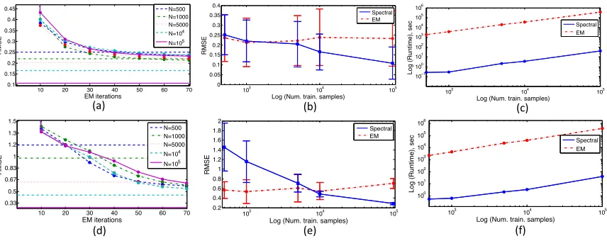
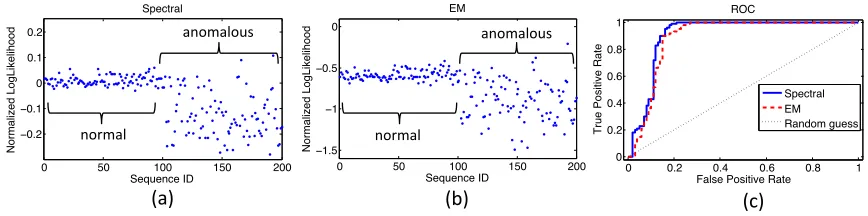
In experiments, comparing our method with EM on both synthetic and real data sets, two obser-vations stand out: (i) the spectral method gets similar or better performance than EM as the number of samples increases, and (ii) the spectral method is orders of magnitude faster than EM for the datasets we consider.
Few remarks are in order about the proposed algorithm. Note that our method does not estimate model parameters explicitly but rather learns alternative representation to perform inference on ob-servable variables. The idea of the obob-servable representations was first introduced with the name ‘observable operators models’ by (Jaeger, 2000) in the context of constructing learning algorithm for the identification of linearly dependent processes. Our formulation cannot be directly used to infer hidden states, although methods such as in (Mossel and Roch, 2005) can be potentially uti-lized to recover original HSMM parameters from the learned representation. Finally, we note that the similar ideas of using homogeneity of HMMs to improve algorithm’s efficiency has also been utilized in other related works, e.g., (Siddiqi et al., 2010; Hsu et al., 2012).
The rest of the paper is organized as follows: We introduce notation in Section 2. In Sec-tion 3, we present HSMM inference from a tensor product perspective and in SecSec-tion 4 introduce the spectral algorithm for inference. In Section 5, we present a careful technical analysis to establish logarithmic dependence of the number of modes in the tensor on maximum latent state persistence. We present experimental results in Section 6 and conclude in Section 7.
2. Notation and Preliminaries
In this section, we cover basic facts about tensor algebra. Detailed tutorials on tensors can be found in (Kiers, 2000) or (Kolda and Bader, 2009). A tensor is defined as a multidimensional array of data, which will be denoted by boldface Euler script letters, e.g., X
m1,...,mN ∈R
Im1×···×ImN, which
isN-mode tensor of dimensions Im1 × · · · ×ImN. A specific mode is denoted by the subscript
variablemi, whose dimension isImi.
Any tensor can be matrisized (or flattened) into a matrix. This mapping can be done in multiple ways, the only requirement is that the number of elements is preserved and the mapping is one-to-one. If we split the modes into two disjoint sets, one corresponding to rows and the other to columns, e.g.,{m1, . . . , mN}={p1, . . . , pK} ∪ {q1, . . . , qL}, then a matrisization ofXis denoted
by a corresponding capital boldface letter, e.g., X
p1,...,pKq1,...,qL∈R
Ip1···IpK×Iq1···IqL.
Tensor Multiplication. Multiplication of two tensors is performed along specific modes. For this, we flatten each tensor to a matrix, perform the usual matrix multiplication and transform the result back to a tensor. The multiplication is denoted by a symbol × with an optional subscript representing the modes along which the operation is performed, e.g.,:
Z
p1,...,pK,r1,...,rM
= X
p1,...,pK,q1,...,qL×q1,...,qL
Y
q1,...,qL,r1,...,rM
,
where Y
q1,...,qL,r1,...,rM ∈ R
Iq1×···×IqL×Ir1×···×IrM and the resulting tensor on the left hand side is
of the form Z
p1,...,pK,r1,...,rM ∈ R
Ip1×···×IpK×Ir1×···×IrM. Observe that in the above, we can flatten
the tensorsXandYin multiple different ways as long as the matrix multiplication remains valid. For example, we could assign the multiplication modes in both tensors to columns, in this case the matrix product becomesZ = XYT. Alternatively, the tensorY could be matrisized with the
X
p,q,r∈R
Ip×Iq×Ir N-mode tensor of dimensionsI
p×Iq×Ir
X
p,q,r∈R
IpIq×Ir Matricization of tensor X
p,q,rwithIpIqrows andIrcolumns
X
p,q,r×rr,s,tY Multiplication of tensorp,q,rX and tensorr,s,tY along moder
X
p,q,r×q,rp,q,rX
−1= I
p,p=Ip Inversion of tensorp,q,rX with respect to modesqandr
Xt Representation of a clique in a Junction tree
ot∈ {1, . . . , no} Observation variable in HSMM
xt∈ {1, . . . , nx} Latent state variable in HSMM
dt∈ {1, . . . , nd} Latent duration variable in HSMM
ORt :={ot+1, ot+2, . . .} Set of observations to the right of time stept
OLt :={. . . , ot−2, ot−1} Set of observations to the left of time stept
Table 1: Summary of some of the key notations used throughout the paper.
An important fact about tensor multiplication is that in a series of tensor multiplications the order is irrelevant (i.e., it is an associative operation) as long as the multiplication is performed along the matching modes, e.g,
X
sp×s
Y
tr×rZrs
=
X
sp×sZrs
×rY
tr.
If we let the matrisized tensors to beX∈RIp×Is,Y∈RIt×Ir andZ∈RIr×Is, then the above can
be verified to be true since
X(YZ)T = XZTYT.
To reduce clutter, in many places we will drop the multiplication subscripts. The implied modes of multiplication can then be inferred from the subscripts of the tensors. Specifically, when two tensors are multiplied, we first check their modes and then multiply along the modes which are common to both of them. For example, in the product X
pqr ×qsrY, the implied multiplication is
performed along the common modes, i.e.,qandr.
Tensor Inversion. We also discuss the operation of tensor inversion. Tensor inverse X−1 is always defined with respect to a certain subset of modes and can be written as follows:
X
p1,...,pK,q1,...,qL×
q1,...,qL X −1
p1,...,pK,q1,...,qL
= I
p1,...,pK,p1,...,pK
,
where the inversion is performed along the modesq1, . . . , qL, and I p1,...,pK,p1,...,pK
denotes an
iden-tity tensor, whose elements are everywhere zero, exceptI(i1, . . . , iK, i1, . . . , iK) = 1. To perform
inversion, we first convert tensor to a matrix, i.e., matrisized tensor. If the modes to be inverted along are associated with columns of the matrix, we compute the right matrix inverse, so that these modes get eliminated after the product. Otherwise, if those modes associated with rows, we com-pute left matrix inverse. Obviously, for the full rank square matrices both choices would produce the same result. For example, in the above equation the matrisized tensor might be of the form
X
p1,...,pKq1,...,qL ∈ R
the modesq1, . . . , qLare eliminated. If the matrisizedXhas full row rank, then the inverse can be
computed, otherwise we could only compute its pseudo-inverse. Tensorizing the matrixX−1gives
us the desired tensor inverse.
Mode Duplication. Observe that in the above, the tensor I
p1,...,pK,p1,...,pK
has duplicate modes.
In general, if a tensor has duplicate modes, the corresponding sub-tensor can be interpreted as a hyper-diagonal. For example, if for a tensor X
pq we construct a tensor pppqX , which has its mode
p duplicated three times, then for a fixed index i, the sub-tensor X(:,:,:, i) is a hypercube with elementsX(:, i)on the diagonal.
Mode duplication enables us to multiply several tensors along the same mode. For example, if we need to multiply tensorsX
sp,prYandZtpalong the modep, then a simple product of the form
X
sp×pprY×pZtp
cannot be done since any product of two tensors along the modep would eliminate it, preventing any further multiplications. In general, if there areN multiplications along the specific mode, then there are must be cumulatively2N number of times such a mode is encountered in the participating tensors. In our example, we might duplicate the modepin, say, tensorZto have
X
sp×p
Y
pr×ptppZ
=X
sp×pWprt=srtV,
so that there are two multiplications over mode p and cumulatively there are four times such a mode is encountered in the participating tensors. To reduce clutter, we sometimes do not explicitly show the duplicated variables in the subscripts; the implied mode repetition will be evident from the context or explicitly stated in cases when there is a confusion. For example, the identity tensor will often be written as I
p1,...,pK
.
Tensor rankFinally, we discuss the meaning of a tensor rank. A tensor can have multiple ranks and each of them is defined based on the rank of a particular matricization. For example, consider a tensor X
pqs. If we flatten it to a matrixX∈R
Ip×IqIs then it can have a rankr
1. On the other hand,
a matricization of the form X ∈ RIpIq×Is can have a rank r
2, and so on. In our derivations, the
particular rank we are referring to will be evident from the context.
In Table 2 we summarized some of the key notations used throughout the paper.
3. Problem Formulation
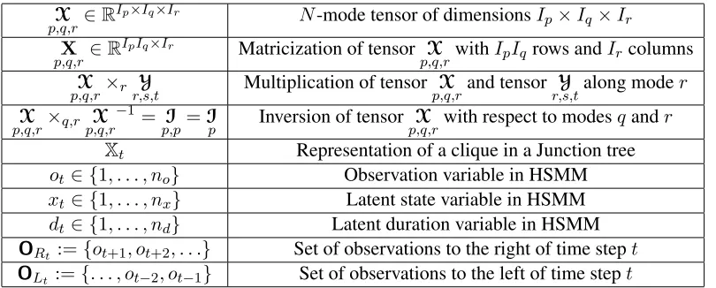
In this paper, we consider the problem of inference in HSMM1(see Figure 1). Unlike the popular HMM, which has a geometric probability for state persistence, i.e., the probability of persisting in the same state overttime steps decreases as πt, whereπ is the probability of persistence for one
time step, HSMM explicitly models state persistence. From a graphical model perspective, HSMM has three sets of variables: the observationsot∈ {1, . . . , no}, the latent statesxt∈ {1, . . . , nx}, and
another latent variabledt ∈ {1, . . . , nd}which determines the length of state persistence. HSMM
1. To reduce clutter, in the main paper we only consider the model for a general time stamptand ignore the initial
(t= 0) and final (t=T) steps of the model, whose representation differs slightly from what is shown in Figure 1.
x
to
td
td
t−1x
t−1o
t−1o
t−2x
t−2d
t−2Figure 1: Hidden Semi-Markov Model (HSMM) depicted as a dynamic Bayesian network. Here
ot∈ {1, . . . , no}denotes an observation at time stept,xt∈ {1, . . . , nx}is a latent state
anddt∈ {1, . . . , nd}is the length of state persistence at time stept.
is specified by three conditional probability tables (CPTs): the observation/emission probability p(ot|xt)and the state transition and the duration probabilities given by
p(dt|xt, dt−1) = (
p(dt|xt) ifdt−1= 1
δ(dt, dt−1−1) ifdt−1>1,
(1)
p(xt|xt−1, dt−1) = (
p(xt|xt−1) ifdt−1= 1
δ(xt, xt−1) ifdt−1>1,
(2)
whereδ(a, b)denotes the Dirac delta function:δ(a, b) = 1ifa=band 0 otherwise. In addition, one can consider suitable prior probabilitiesp(x0)andp(d0). In essence,dt works as a down counter
for state persistence. Whendt−1 >1, the model remains in the same statext=xt−1, while when
dt−1 = 1, one samples a new statext and the new duration in that statedt|xt. For our analysis,
we assumep(dt|xt, dt−1 = 1)to be a discrete distribution over{1, . . . , nd}wherenddenotes the
largest duration of state persistence.
The considered inference problem can be posed as follows: given a set of discrete sequences
{S1, . . . ,SN} drawn independently from the HSMM model, where each sequence is defined as
Si ={oi
1, . . . , oiTi}, i= 1, . . . , N, our goal is to compute the probabilityp(S
test)of any given test
sequenceStest = (otest
1 , . . . , otestT ). A traditional approach would be to estimate the CPTs using
the EM algorithm, and use the estimates to computep(Stest). However, the EM algorithm is not
guaranteed to estimate the parameters optimally, and hence the computation ofp(Stest) may be
incorrect. The focus of our work is to develop a provably correct spectral algorithm for computing the probabilityp(Stest).
3.1 HSMM in Tensor Notations
We start by considering the matrix forms of the HSMM parameters and writing the computations in tensor notation, as introduced in Section 2. Specifically, p(dt|xt, dt−1 = 1) is denoted as
D ∈ Rnd×nx, p(x
t|xt−1, dt−1 = 1)is denoted asX ∈ Rnx×nx, andp(ot|xt) asO ∈ Rno×nx.
otxt
xt
dtxtdt−1
xtxt−1dt−1
dt−1xt−1dt−2 xtdt−1
xt−1dt−2
xt−1xt−2dt−2
xt−1
ot−1xt−1 Ot
Xt
Dt
Ot−1
Xt−1
xt−1dt−1
Dt+1
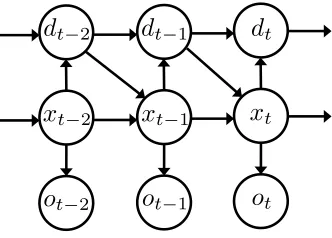
Figure 2: Junction Tree for Hidden Semi-Markov Model. The ovals represent cliques, which are denoted by capital blackboard bold variables; the rectangles denote separators. Symbols within the shapes represent the variables on which the corresponding potentials depend.
Assumptions
A1. Xis full rank and has non-zero probability of visiting any state from any other state. A2. Dhas a non-zero probability of any duration in any state.
A3. Ois full column rank and, as a consequence,nx≤no.
We provide some comments on the above assumptions. We note that the assumptionA1can be relaxed to allow zero entries (while still ensuring full rank structure) and thus prevent certain states to be directly reachable from other states; however, this would require more involved analysis based on the mixing time of the corresponding Markov chain (Levin et al., 2009), and is not pursued in this work. Also, observe that the assumption ofnx ≤no is needed in order to ensure that hidden
states are identifiable, although recent work is showing that such an assumption can be relaxed in some cases (Bailly et al., 2009; Anandkumar et al., 2013b). Intuitively, it means that the number of different observations coming from each state is large enough, so that one hidden state can be differentiated from the other.
To express the joint probabilityp(o1, . . . , oT)for any possible observation sequence in tensor
form, we utilize the junction tree algorithm (Barber, 2012). The resulting tree is shown in Figure 2 and it corresponds to the graphical model of HSMM in Figure 1. Recall, that the junction tree is a tree-structured representation of an arbitrary graph enabling efficient inference. It can be constructed by forming a maximal spanning tree from the cliques of the graph. The cliques then represent vertices in the junction tree and the edges connecting the vertices are labeled with variables common to two cliques it connects. The set of variables on the edges are referred to as separators. For example, in Figure 2 the cliques Xt andDt have two variables in common, xt−1 and dt−1, and
which define the sepatator betweenXtandDt.
We proceed by representing the clique CPTs of the junction tree as tensors. For example, the cliqueXt, containing the CPT ofp(xt|xt−1, dt−1)is represented as tensor X
xt|xt−1dt−1
. For ease of
exposition, the tensor’s modes are named based on the variables on which the tensor depends. We also keep the conditioning symbol|for clarity. Similarly, we represent the cliqueDtwith its CPT
p(dt|xt, dt−1)as tensor D
dt|xtdt−1
, andOtcontainingp(ot|xt)as tensor O ot|xt
.
If we denote the joint probability of the observed sequence p(o1, . . . , oT) as P o1,...,oT
then the
P
o1,...,oT
=Y t
D
dt−1|xt−1xt−1dt−2
×xt−1dt−1
X
xtxt|xt−1dt−1dt−1
×xt O
ot|xt
, (3)
where, for simplicity, we denoted byQtthe tensor product over multiple time steps.
Note that in (3) the neighboring tensors are multiplied along the modes which are the separator variables between two corresponding neighboring cliques in Figure 2. Therefore, as we discussed in Section 2, if a certain mode of a tensor is to participate multiple times in products with other tensor, the mode must be duplicated for the expression to remain correct. It can easily be seen from the junction tree that the number of times the mode is duplicated depends on the number of times such a variable appears in separators adjacent to the clique. For example, the tensor X
xtxt|xt−1dt−1dt−1
has
a modext−1 appearing once in the separator connectingXtandDtin Figure 2, whilextappears a
total of two times, once in the separator connectingXtandOt, and once in the separator connecting
XtandDt+1. Finally,dt−1 appears in the separator betweenDtandXt, and betweenDt+1andXt.
Applying the same reasoning to tensorsDandOresults in the expression (3).
3.2 Summary of Technical Results
In this work, we represent expression (3), which is defined in terms of unknown model parameters, in a differentobservable form, where all the factors can be estimated directly from data using certain sample moments without knowledge of model parameters. Such an observable form is derived in Sections 4.1 and 4.2. Based on the observable form, in Section 4.3 we propose a simple spectral algorithm which requires estimatingX,DandOfor all the time stampst. This estimation process is expensive as it involves costly tensor operations to be performed at each time indext. Moreover, the accurate estimation of these tensors requires large number of training sequences which might not be available, leading to inaccurate and unstable computations. However, exploiting the homogeneity property of HSMMs, i.e., the probability distributions represented by the above tensors are the same across all time t, we derive a computationally efficient and accurate spectral algorithm in Section 4.4 which requires the estimation of only three tensors for all the time stamps t. Although the computational complexity of the inference, i.e., the evaluation of expression (3), is not affected by the introduced modifications, the overall algorithm becomes faster and more accurate.
In Section 5 we return to the results of Sections 4.1 and establish the conditions under which the derived observable form can be computed from data. In particular, our analysis shows that the number of dimensions of the required sample moments (in the form of tensors, estimated from data and representing the co-occurrence frequency of certain observable variables), has logarithmic dependence on the longest state persistence nd. Such conclusion is in contrast to the analysis,
which would follow from the work of (Parikh et al., 2012), in which case the required number of dimensions in the estimated sample moments would have had linear dependence on nd. The
4. Spectral Algorithm for Inference in HSMM
In this Section we present the details of the spectral inference approach. In particular, in Sections 4.1 and 4.2 we derive observable tensor representation and show how to estimate each of its factors directly from data. Practical algorithms implementing these ideas are then derived in Sections 4.3 and 4.4.
4.1 Observable Tensor Representation
Observe that the computation of the joint probability in (3) requires knowledge of the unknown model parameters. Our goal is to change the tensor representation such that P
o1,...,oT
can be written
in terms of the quantities directly computable from data. To that end, we follow (Parikh et al., 2012) and between every two factors in (3) introduce an identity tensor with the modes corresponding to the modes along which the multiplication is performed. For example, consider a part of (3) after introducing identity tensors:
× I
xt−1dt−2×
xt−1dt−2 D dt−1|xt−1xt−1dt−2
×xt−1dt−1 I
xt−1dt−1× xt−1dt−1
X xtxt|xt−1dt−1dt−1
×xtI
xt×
xt O
otxt
×xtdt−1 I
xtdt−1×
, (4)
where all the identity tensors have duplicated modes which are not shown.
Now rewrite each of the identity tensors in (4) as a multiplication of some factor times its inverse. For example,
I
xt
= F
ωxtxt×ωxt
F−1
ωxtxt
,
for some invertible factor F
ωxtxt
, whose modes arextandωxt. Note that the choice of modextis
fixed and is determined by the modes of the identity tensor I
xt
, while the modeωxt is not fixed and
we have freedom in selecting it as convenient. Moreover, observe that since the tensor inversion is done along the mode ωxt and the matrixFhas its rows associated with modeωxt, we need to
ensure such a matrix has full column rank for the inverse to exist and for the productF−1Fto be the
identity matrix (see Section 2 for more details on tensor inversion). Based on the above discussion, we choose tensorFsuch that (i)ωxt are the observed variables, (ii) F
ωxtxt
is invertible, i.e., matrix
F, whose columns correspond toxt, has full column rank, and (iii) we interpret the factor F ωxtxt
as
corresponding to a conditional probability distribution, i.e.,p(ωxt|xt)and therefore write F
ωxt|xt
.
After expanding each of the identity tensors, regrouping the factors and recalling that in a series of tensor multiplication the order is irrelevant, we can identify three modified tensors:
˜
D
ωxt−1dt−2ωxt−1dt−1 = F
−1
ωxt−1dt−2|xt−1dt−2
×xt−1dt−2 D dt−1|xt−1xt−1dt−2
×xt−1dt−1 F ωxt−1dt−1|xt−1dt−1 ˜
X
ωxt−1dt−1ωxtωxtdt−1
= F−1
ωxt−1dt−1|xt−1dt−1
×xt−1dt−1
X
xtxt|xt−1dt−1dt−1
×xt F
ωxt|xt
×xtdt−1 F ωxtdt−1|xtdt−1 ˜
O
ωxtot
= F−1
ωxt|xt
×xt O
ot|xt
.
tensors from data. The right hand side in the above expressions depend on the unknown model parameters, whereas the tensors on the left do not correspond to valid probability distributions (due to the presence of inversesF−1), and so cannot be estimated from data using sample moments. For
example, D˜
ωxt−1dt−2ωxt−1dt−1 is not a tensor form ofp(ωxt−1dt−2, ωxt−1dt−1).
Next, we discuss the choice of the observable set ω in the factorsF. From Figure 2 we can see that there are three types of separators which depend onxt−1dt−1,xtdt−1andxt, consequently,
there are three types of identity tensors which we introduced in (4), i.e., I
xt−1dt−1
, I
xtdt−1
and I
xt
.
Therefore, we need to define three types of observable setsωxt−1dt−1,ωxtdt−1 andωxt. There are
multiple choices for these sets, one of them is ωxt−1dt−1 = ωxtdt−1 = {ot+1, ot+2, . . .} for all
t(see Figure 3 for an illustration). Ideally, we want these sets to be of minimal size, since they need to be estimated from observations. The detailed description of how many and which of these observations to select to get a minimal set is deferred until Section 5, where we also show that we can setωxt =ot.
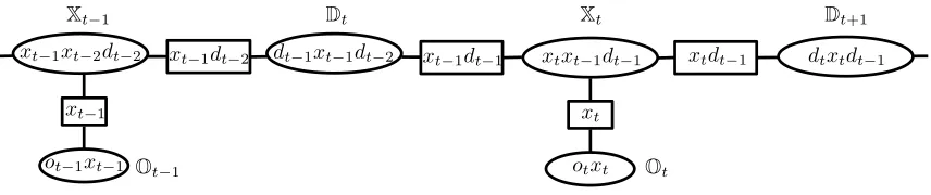
In what follows, we defineORt :={ot+1, ot+2, . . . , ot+τ}(see Figure 3) to emphasize that this
is a fixed set of observations whose lengthτ is yet to be determined, starting after time stamptand going to the right (or forward in time) in the graphical model in Figure 1. With these definitions, settingωxt−1dt−1 = ORt, ωxtdt−1 = ORt,ωxt−1dt−2 = ORt−1 andωxt = ot, we can now rewrite
(3) in the form:
P
o1,...,oT
=Y t
˜
D
ORt−1ORt×ORt
˜
X
ORtotORt×
ot O˜
otot
. (5)
Comparing (3) and (5) we see that the above equation expresses the joint probability distribution in the observable form. As noted above, we cannot yet use this formula in practice since we do not know how to compute the transformed tensors. In what follows, we show how to estimate such tensors directly from data, without the need for the model parameters.
4.2 Estimation of Observable Tensors
In this Section we express each of the tensors in (5) in forms which can be directly estimated from the observed sequences.
4.2.1 COMPUTATION OFTENSOR D˜ ORt−1ORt
Consider the tensor from Section 4.1
˜
D
ORt−1ORt= F
−1
ORt−1|xt−1dt−2×
xt−1dt−2 D
dt−1|xt−1xt−1dt−2×
xt−1dt−1 F
ORt|xt−1dt−1
, (6)
whose modes are the observable variablesORt−1 andORt. To estimate this tensor from data,
con-siderOLt−1, a set of the observed variables such thatOLt−1andORt−1are independent, conditioned
onxt−1dt−2 (see Figure 3):
p(OLt−1,ORt−1) =
X
xt−1dt−2
xt
xt−1
xt−2 xt+1
dt−2 dt−1 dt dt+1
ot−2 ot−1 ot ot+1
ORt
ORt−1
OLt−1
OLt
Figure 3: Conditional independence in HSMM. The figure depicts two sets of relationships: OLt
and ORt are independent conditioned on xt−1dt−1, similarly, OLt−1 and ORt−1 are
conditionally independent given xt−1dt−2. We defined OLt = {. . . , ot−2, ot−1} and ORt ={ot+1, ot+2, . . .}.
The above conditional independence relationship can be written in tensor form:
M
OLt−1ORt−1=OLt−1|Fxt−1dt−2×
xt−1dt−2 F
ORt−1|xt−1dt−2×
xt−1dt−2 K xt−1dt−2
, (8)
where tensorK represents the marginal p(xt−1, dt−2). Note that, though not shown, the modes
xt−1anddt−2need to appear twice inK, since it interacts with both other terms (see the discussion
on mode duplication in Section 2). The setOLt−1 is defined in a way similar toORt but with the
set of observations starting at time stampt−2 and going to the left (or backward in time), i.e.,
OLt−1 :={. . . , ot−3, ot−2}(see Figure 3).
Next, we express the inverse of the tensor F
ORt−1|xt−1dt−2
from (8) and substitute back to (6). For
this, we observe that in (6) the tensorF−1is inverted with respect to modeORt−1, therefore, we do
the following:
M
OLt−1ORt−1×ORt−1 F
−1
ORt−1|xt−1dt−2
= F
OLt−1|xt−1dt−2
×xt−1dt−2 I xt−1dt−2×
xt−1dt−2 K xt−1dt−2
F−1
ORt−1|xt−1dt−2
= M−1
OLt−1ORt−1×OLt−1 O F
Lt−1|xt−1dt−2
×xt−1dt−2 K xt−1dt−2
, (9)
where M−1
OLt−1ORt−1 is inverted with respect to modeOLt−1. Next, substituting (9) back to (6), we get
˜
D
ORt−1ORt= M
−1
OLt−1ORt−1×OLt−1O F
Lt−1|xt−1dt−2
×xt−1dt−2 K xt−1dt−2×
xt−1dt−2 D dt−1|xt−1xt−1dt−2
×xt−1dt−1 F
ORt|xt−1dt−1 = M−1
OLt−1ORt−1 ×OLt−1 O M
Lt−1ORt
, (10)
where we have eliminated all the latent variables by multiplying the last four terms on the first line. Observe that the tensors M
OLt−1ORt−1 andOLtM−1ORtrepresent valid joint probability distributions
˜
O otot
˜
O ot−1ot−1
ot
ot−1
�
M ot−1ot
−1× M ot−1ot
� �
M otot+1
−1× M otot+1
� �
M
OLtORt
−1× M OLtORtot
� �
M
OLt−1ORt−1
−1× M OLt−1ORt
� �
M
OLtORt
−1× M OLtORt+1
� �
M
OLt−1ORt−1
−1× M
OLt−1ORt−1ot−1
�
˜
X
ORt−1ot−1ORt−1 ORt−1
˜
X
ORtotORt
ORt
˜
D
ORt−1ORt
˜
D
ORtORt+1
ORt
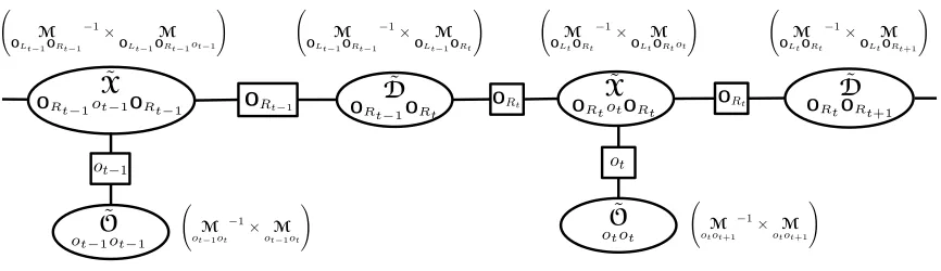
Figure 4: Graphical representation of the HSMM spectral algorithm for inference in Algorithm 1. As compared to junction tree in Figure 2, the cliques and separators are now defined in terms of the tensors, which are defined with respect to the observed data. The expressions in the parenthesis show the observable representation of the corresponding tensors.
defined with respect to unknown model parameters (as, for example, in (7)), we can readily estimate them from data. For example, M
OLt−1ORtis a tensor, where each entry is computed from the frequency
of co-occurrence of tuples of the observations{. . . , ot−3, ot−2, ot+1, ot+2, . . .}. Ideally, we want a
small number of observations since we need to estimate their co-occurrence frequency from the training data. A precise characterization of how many and which of these observations suffices for the analysis will be done in Section 5.
4.2.2 COMPUTATION OFTENSOR X˜ ORtotORt
The form of this tensor was established at the beginning of Section 4.2 to be:
˜
X
ORtotORt
= F−1
ORt|xt−1dt−1
×xt−1dt−1
X
xtxt|xt−1dt−1dt−1
×xt F
ot|xt
×xtdt−1 F
ORt|xtdt−1
. (11)
Consider the following conditional independence relationship (see Figure 3):
M
OLtORt=OLt|xFt−1dt−1×
xt−1dt−1 F
ORt|xt−1dt−1×
xt−1dt−1 K xt−1dt−1
, (12)
where K
xt−1dt−1
= K
xt−1dt−1xt−1dt−1
and we omitted the duplicated modes.
We express the inverse of tensor F
ORt|xt−1dt−1
from the above equation
F−1
ORt|xt−1dt−1
= M−1
OLtORt×OLt OLt|xFt−1dt−1
×xt−1dt−1 K xt−1dt−1
,
where tensor F
ORt|xt−1dt−1
is inverted with respect to modeORt, while M
OLtORtis inverted with respect
to modeOLt. Substituting back to (11), we get
˜ X
ORtotORt
= M−1
OLtORt×OLt OLt|xFt−1dt−1
×xt−1dt−1 K
xt−1dt−1×
xt−1dt−1
X xtxt|xt−1dt−1dt−1
×xt F
ot|xt
×xtdt−1 F
ORt|xtdt−1
Considering the last five factors and multiplying them together, we obtain
M
OLtORtot
= F
OLt|xt−1dt−1
×xt−1dt−1 K xt−1dt−1×
xt−1dt−1
X
xtxt|xt−1dt−1dt−1
×xt F
ot|xt
×xtdt−1 F
ORt|xtdt−1
.
Finally, (11) can now be written as
˜
X
ORtotORt
= M−1
OLtORt×OLt OLtMORtot
, (13)
where the right hand side can now be estimated directly from data, without the need for the model parameters.
4.2.3 COMPUTATION OFTENSOR O˜
otot
Finally, we consider the tensor
˜
O
otot
=F−1
ot|xt
×xt O
ot|xt
. (14)
The conditional independence relationship can take the form
M
otot+1 = F
ot|xt
×xt F
ot+1|xt ×xtKx
t
.
Expressing the inverse of F
ot|xt
F−1
ot|xt
=M−1
otot+1×ot+1
F
ot+1|xt ×xtKx
t
,
and substituting in (14), we get
˜
O
otot
=M−1
otot+1×ot+1
F
ot+1|xt ×xtK
xt ×xt
O
ot|xt
=M−1
otot+1×ot+1
M
otot+1
. (15)
4.3 Basic Version of Spectral Algorithm
The basic version of the spectral HSMM algorithm to compute P
o1,...,oT
entirely using the observed
variables can be described as a two step process: in the learning step, compute tensors D˜
ORt−1ORt,
˜
X
ORt−1otORt
, and O˜
otot
for eachtusing (10), (13) and (15) from the training data. In the inference step,
use (5) to computep(Stest). Algorithm 1 shows its basic version and Figure 4 shows the graphical
representation of this algorithm in terms of the transformed junction tree of Figure 2.
As an example, consider the learning step of the algorithm and the computation of tensor in (10), i.e.,
˜
D
ORt−1ORt = M
−1
OLt−1ORt−1×OLt−1 O M
Lt−1ORt
Algorithm 1Basic Spectral Algorithm for HSMM inference
Input:Training sequences:Si ={oi
1, . . . , oiTi}, i= 1, . . . , N.
Testing sequence:Stest ={otest
1 , . . . , otestT }. Output: p(Stest)
Learning phase: for alltdo
Estimate D˜
ORt−1ORt,
˜
X
ORtotORt
and O˜
otot
from data{S1, . . . ,SN}using equations (10), (13) and
(15).
end for
Inference phase:
p(Stest) = 1
fort=T down tot= 1do
p(Stest) =p(Stest)× D˜
ORt−1ORt×ORt
˜
X
ORtotORt×
ot O˜
otot
ot=otestt
end for
For a fixedt, we estimate each entry of M
OLt−1ORt−1 from the frequency of co-occurrence of tuples
of the observed symbols{. . . , ot−3, ot−2, ot+1, ot+2, . . .}in the given data set (the setsOLt−1 and ORt−1 were defined at the beginning of Section 4.2). Next, following our discussion after (9),
we invert M−1
OLt−1ORt−1 along the modesOLt−1. For this, we matrisize the tensor so that the modes
OLt−1 are associated with columns andORt−1 with rows in matrix M
ORt−1OLt−1 (see Section 2 for
the discussion on tensor matrisization and inversion). Finally, we compute the right inverse of the matrix to obtain M−1
ORt−1OLt−1, so thatORt−M1OLt−1 · M
−1
ORt−1OLt−1 =I
Similarly, we estimate the tensor M
OLt−1ORt using the corresponding co-occurrences of the
ob-served symbols. Matrisizing the result, so that the rows correspond to the modes OLt−1 and the
columns toORt, we get the matrix M
OLt−1ORt. The multiplication M
−1
ORt−1OLt−1 · OLtM−1ORt =
˜
D ORt−1ORt
produces a matrix, which is then converted to a tensor to get the final result in (10).
In the inference step we perform tensor multiplications for eachtrunning along the length of the testing sequence. The only nuance here is that before multiplying the tensor O˜
otot
with others,
the second modeot, whose dimension isnois collapsed into a scalar. This operation is denoted as ˜
O
otot
ot=otestt
, which means that based on the value of thetth symbol in testing sequence, we select
the column corresponding to the elementotest
t . For example, ifoO˜
tot ∈ R
10×10andotest
t = 3then
˜
O
otot
ot=otestt
∈R10×1, a third column in the original matrix.
Analyzing (10), (13) and (15), we see that the computational complexity of the learning phase of the algorithm is determined by the tensor inverses and multiplications. For example, if in (10) we de-note|OR|=|OL|=`(in Section 5 we will show that`=d1 +loglognndxe), then M
OLt−1ORt−1 ∈R
and M
OLt−1ORt∈R
n`
o×n`o. The computational complexity of the multiplications and inversions would
then be O(n3`
o ). Performing this computations for all tand assuming that the length of the
se-quences isT, would result inO n3` o T
. Additionally, withNtraining examples there will be a cost ofO(`N T)to estimate the sample momentsM, which is based on counting the co-occurrences of certain observable symbols. In the inference phase of the algorithm, we perform a series of tensor multiplications with the cost ofO(n3`
o T).
4.4 Efficient Version of Spectral Algorithm
Note that for large`the accurate estimation of tensorsMfor eachtwill require large number of training sequences which might not be available, leading to inaccurate and unstable computations. Observe, however, that for example the estimated sample-based tensors M
OLt−1ORt in (10) for eacht
estimate the same population quantity due to homogeneity of HSMM. Thus, a novel aspect of our work is the improvement of the accuracy and efficiency of the basic Algorithm 1 by exploiting the homogeneity property of HSMM and estimating the tensorsX,˜ D˜ andO˜ using all time steps, i.e., by pooling samples across differenttand averaging the estimates. Thus, we compute only three tensors across allt, as opposed to computing these tensors separately for eacht.
We show the details for computing the tensors D˜ in the batch form. The derivations for other tensorsX˜ andO˜ can be computed in a similar manner. Recall from (10) the form of D˜
ORt−1ORt, and
consider the following alternative expression, based on the sum over allt:
˜
D= X
t
M
OLt−1ORt−1
!−1 ×OL
X
t
M
OLt−1ORt
!
, (16)
whereOLdenotes a generic mode of the averaged tensorM, corresponding toOLt−1for allt. Note
that in practice, instead of summation, we use averaging to avoid numerical overflow problems, and the average is equivalent to the expression in (16) since the term T1 cancels out. Since
M
OLt−1ORt−1=OLt−1|Fxt−1dt−2×
xt−1dt−2 F
ORt−1|xt−1dt−2×
xt−1dt−2 K xt−1dt−2
, (17)
the first term inside brackets can be rewritten as:
X
t
F
OLt−1|xt−1dt−2×
xt−1dt−2 F
ORt−1|xt−1dt−2×
xt−1dt−2 K xt−1dt−2
(a)
= X
t
F
ORt−1|xt−1dt−2×
xt−1dt−2 F
OLt−1xt−1dt−2
(b)
= F
OR2|x2d1× X
t
F
OLt−1xt−1dt−2 !
, (18)
where in(a)we combined the two factors, i.e., F
OLt−1xt−1dt−2
= F
OLt−1|xt−1dt−2
×xt−1dt−2 K xt−1dt−2xt−1dt−2
and in(b) we used the homogeneity property of HSMM, i.e., the fact that F
ORt−1|xt−1dt−2
does not
depend on time stampt, and extracted one of the common factors, in fact, the first factor. Note
that the term F
OLt−1xt−1dt−2
, on the other hand, does depend ont since the factor K
xt−1dt−2
, which
Similarly, since
M
OLt−1ORt=OLt−1|xFt−1dt−2
×xt−1dt−2 K xt−1dt−2×
xt−1dt−2 D dt−1|xt−1xt−1dt−2
×xt−1dt−1 F
ORt|xt−1dt−1
,
(19)
rewrite the second term in (16) as
X
t
F
OLt−1|xt−1dt−2
×xt−1dt−2 K xt−1dt−2×
xt−1dt−2 D dt−1|xt−1xt−1dt−2
×xt−1dt−1 F
ORt|xt−1dt−1 =X
t
F
OLt−1xt−1dt−2×
xt−1dt−2 D dt−1|xt−1xt−1dt−2
×xt−1dt−1 F
ORt|xt−1dt−1
= X
t
F
OLt−1xt−1dt−2
!
× D
d2|x2x2d1
×x2d2 F
OR3|x2d2
, (20)
where we used the transformations similar as in (18), i.e., the fact that the factors D
dt−1|xt−1xt−1dt−2
and F
ORt|xt−1dt−1
are homogeneous, independent oft. Now if we multiply the inverse of (18) with
(20), we get
F−1
OR2|x2d1
× X
t
F
OLt−1xt−1dt−2
!−1
× X
t
F
OLt−1xt−1dt−2
!
× D
d2|x2x2d1
× F
OR3|x2d2
(21)
= F−1
OR2|x2d1
×x2d1 D d2|x2x2d1
×x2d2 F
OR3|x2d2 = D˜
OR2OR3
= D˜
ORt−1ORt, (22)
where in (21) we used the fact that the order in which tensors are multiplied is irrelevant and also the fact that the terms in parenthesis are invertible. This is due to the fact that the set of observations
OLt−1for alltis selected so as to make each of the summand invertible (see Section 5 for the details
about the choice ofOLt−1). Moreover, in (22) we used the definition of D˜
ORt−1ORt
˜
D
ORt−1ORt= F
−1
ORt−1|xt−1dt−2
× D
dt−1|xt−1dt−2
× F
ORt|xt−1dt−1
,
together with the homogeneity property of HSMM. We note that although the above derivations rely on the assumption of the existence of the matrix summation inverse in equation (21), the idea of ag-gregating observations from multiple time steps has also been utilized by other works, e.g., (Siddiqi et al., 2010; Anandkumar et al., 2014a) and shown to be very effective in practice, significantly improving the accuracy of corresponding algorithms.
We can conclude that the batch form of the tensor takes the form:
˜
D= X
t
M
OLt−1ORt−1
!−1 ×OL
X
t
M
OLt−1ORt
!
Algorithm 2Efficient Spectral Algorithm for HSMM inference
Input:Training sequences:Si ={oi
1, . . . , oiTi}, i= 1, . . . , N.
Testing sequence:Stest ={otest
1 , . . . , otestT }. Output: p(Stest)
Learning phase:
EstimateD˜,X˜ andO˜ from data{S1, . . . ,SN}using equations (23), (24) and (25). Inference phase:
p(Stest) = 1
fori=T down toi= 1do
p(Stest) =p(Stest)×D˜ ×X˜ ×O˜|
o=otest i
end for
Similar derivations can be carried out to obtain the rest of the tensors in the batch form:
˜
X= X
t
M
OLtORt
!−1 ×OL
X
t
M
OLtORtot !
, (24)
˜
O= X
t
M
otot+1
!−1 ×o
X
t
M
otot+1
!
. (25)
where in the last expression the modeo corresponds to the mode ott+1 after averaging of tensor
M
otot+1
for allt.
Analyzing (23), (24) and (25), we see that the computational complexity of the learning phase of the Algorithm 2 is nowO (n2`
o +`N)T
, mainly determined by the tensor additions and the estimation of the sample momentsM. The number of inverses and multiplications is now fixed and independent of sequence lengthT. Specifically, there will be only three tensor multiplications and inversions for a total cost of O(n3`
o )(as opposed to T tensor multiplications and inversions as in
Algorithm 1). The computational complexity of the inference phase isO(n3`
o T), which is the same
as for Algorithm 1.
Note that such a batch tensor computation significantly improves the accuracy of the resulting spectral algorithm. In part, this is due to the fact that we now use more data to estimate the tensors as compared to the original form (5). The estimates obtained in this form have lower variance, which in turn ensures that the inverses we compute in (23), (24) and (25) are more stable and accurate.
5. Rank Analysis of Observable Tensors
In Section 4.2.1, when we derived the equations (10), (13) and (15), we glossed over the question of the existence of tensor inverses M−1
OLt−1ORt−1, M
−1
OLtORt andM
−1
otot+1
. In this section, our task is to analyze
the rank structure of these tensors and impose restrictions on the setsOLandORto ensure that the
to get
˜
D
ORt−1ORt= F
−1
ORt−1|xt−1dt−2×
F−1
OLt−1|xt−1dt−2× K−1
xt−1dt−2× K
xt−1dt−2× F
OLt−1|xt−1dt−2×
D
dt−1|xt−1xt−1dt−2× F
ORt|xt−1dt−1
,
where we dropped the multiplication subscripts and some of the duplicated modes, which can be inferred from the context. Observe that in order for the above equation to produce (6), the terms in the middle must multiply out into identity tensor
I
xt−1dt−2
= K−1
xt−1dt−2×
xt−1dt−2 K xt−1dt−2
I
xt−1dt−2
= F−1
OLt−1|xt−1dt−2
×OLt−1 F OLt−1|xt−1dt−2
. (26)
Moreover, recall that F
ORt−1|xt−1dt−2
was originally introduced as part of the identity tensor
I
xt−1dt−2
= F−1
ORt−1|xt−1dt−2
×ORt−1 F ORt−1|xt−1dt−2
, (27)
therefore, we can conclude that for (10) to exist, the identity statements in (26) and (27) must be sat-isfied. These statements have implications for the ranks of K
xt−1dt−2
, F
OLt−1|xt−1dt−2
and F
ORt−1|xt−1dt−2
,
which in turn determine the length of the observation sequencesOLt−1 andORt−1.
Since K
xt−1dt−2
represents a distributionp(xt−1dt−2), its matrisized version is a diagonal matrix
with p(xt−1dt−2) on the diagonal. Using assumptionsA1 and A2, it can be concluded that the
diagonal elements in this matrix are non-zero and it has ranknxnd, it is thus invertible and so the
first equation in (26) is satisfied.
Next, consider the second equation in (26) and recall from Section 2 that if we matrisize the
tensor as F
OLt−1|xt−1dt−2
∈ Rn
|OLt
−1|
o ×nxnd thenFmust have full column rank n
xnd for the proper
inverse to exist, implyingn|OLt−1|
o ≥ nxnd. Similarly, F
ORt−1|xt−1dt−2
in (27) must have ranknxnd.
As a consequence of the above, the tensor
M
OLt−1ORt−1=OLt−1|Fxt−1dt−2
× F
ORt−1|xt−1dt−2
× K
xt−1dt−2
(28)
will have ranknxndand, in general, is rank-deficient.
The argument above can also be used to show that M
OLtORt has rank nxnd since in (12) the
tensors K
xt−1dt−1
, F
OLt|xt−1dt−1
and F
ORt|xt−1dt−1
all have ranknxnd. Similarly, M otot+1
will have ranknx
because in (15) the rank of the participating tensorsK
xt
, F
ot+1|xt
and F
ot|xt
isnx. In particular, note that
the tensor F
ot|xt
is the observation matrixO ∈Rno×nx of the model and it has rankn
xaccording to
assumptionA3. This conclusion also justifies our choice forωxt =otat the end of Section 4.1.
The key unknowns now are the sets of the observed variables OR and OL that must be
ap-propriately selected for the corresponding tensors to have rank nxnd. Recall that we defined
ORt−1 = {ot, ot+1, . . .}. As one of the new key results of our work, we established that if we
select the observationsotnon-sequentially with gaps that grow exponentially with the state sizenx
ot
nd nd
ORt−1
OLt−1
ot+19
ot+17
ot+11
ot−2
ot−13
ot−21ot−19
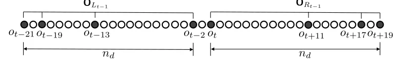
Figure 5: Observations required to estimate M
OLt−1ORt−1 from data for HSMM with nx = 3and
nd= 20.
Theorem 1 Let the number of observations be|ORt−1|=`and define the set of indices
S = maxt, t+ (nd−1)−(nix−1) |i= 0, . . . , `−1 , such thatORt−1 = {ok|k ∈ S}then
the rank of tensor F
ORt−1|xt−1dt−2
ismin[n`
x, nxnd].
As a consequence of this result, to achieve the rank nxnd we will require` = d1 + loglognndxe
observations, since we need to ensuren`
x ≥ nxndand we want the minimal`which satisfies this.
The span of the selected observations is nd, while their number is only logarithmic in nd. For
example, consider the estimation of tensor M
OLt−1ORt−1 for an HSMM withnx = 3 andnd = 20.
In this case`= 4andORt−1 ={ot, ot+11, ot+17, ot+19}andOLt−1 ={ot−21, ot−19, ot−13, ot−2},
where the set OLt−1 is defined similar to ORt−1 in Theorem 1 but for the indices to the left of
time stampt−1. Figure 5 illustrates this example. We note that the requirement for the span of the selected observations to be nd, which is a maximum state persistence, is to ensure that for a
given time stampt, we select the observations far enough to the right and left of it so that those observations are likely to be sampled from different hidden states.
In order to prove the above Theorem, we will focus our analysis on the tensor F
ORt+1|xtdt
instead
of F
ORt−1|xt−1dt−2
. This specific choice was only done to ensure the compactness in our notations,
however the HSMM homogeneity property enables us to transfer this result for tensors for anyt. Note that
F
ORt+1|xtdt
= F
ORt−1|xt−2dt−2
= F
ORt−1|xt−1dt−2×
xt−1dt−2 X xt−1dt−2|xt−2dt−2
,
where the first equality is due to the homogeneity property of the model and in the second equality we embedded the HSMM transition matrix into tensor X
xt−1dt−2|xt−2dt−2
with modedt−2 duplicated.
It can be shown that the matricized tensor X
xt−1dt−2|xt−2dt−2
∈ Rnxnd×nxnd has rankn
xnd, i.e., it is
full rank. Therefore, the rank structure of F
ORt+1|xtdt
determines the rank structure of F
ORt−1|xt−1dt−2
.
The rest of Section 5 is devoted to the proof of Theorem 1. We first establish the rank structure
of tensor F
ORt+1|xtdt
for sequential set of observationsORt+1 and then analyze the rank structure for
5.1 Rank Structure of Tensor F
ORt+1|xtdt
Define byXRt+1 ={xt+2, xt+3, . . .}, the sequence of hidden states corresponding to observations
ORt+1 ={ot+2, ot+3, . . .}. Then using conditional independence property of the graphical model
in Figure 1, namely, that the variablesORt+1andxtdtare independent givenXRt+1, we can write:
F
ORt+1|xtdt
= Q
ORt+1|XRt+1×XRt+1T|xtdt
, (29)
for some tensorsQandT, representing the appropriate probability distributions.
Denoting`=|ORt+1|=|XRt+1|, it can be verified, that the matrisized form ofQin (29) can be
written asQ=⊗`O ∈Rn
`
o×n`x, i.e., a Kronecker product of the observation matrixOwith itself`
times. According to the assumptionA3,rank(O) =nx andnx ≤no, and using the rank property
of the Kronecker product, we infer thatrank(Q) =n` x.
Combining the above conclusion with the fact that the matrisized form of the other two tensors in (29) isF∈Rn`
o×nxndandT∈Rn`x×nxnd, to ensure invertibility ofF, we need to select a set of
variablesXRt+1 so thatrank
T XRt+1|xtdt
= nxndwith the condition thatn`x ≥ nxnd. Thus, the
problem of the analysis of the rank structure of tensor F
ORt+1|xtdt
translates to the problem of rank
structure of matrix T XRt+1|xtdt
. In what follows, we assume thatXRt+1 = {xt+2, . . . , xt+`+1}are
sequential and so we would be interested in determining`which makesrank T XRt+1|xtdt
=nxnd.
Later, the sequential assumption will be removed and we show how to select such variables in a more efficient way.
5.1.1 COMPUTATION OFFACTORT
In order to study the rank structure of T XRt+1|xtdt
we will have to understand the mechanism how
this matrix is constructed and how the rank changes as the size of XRt+1 increases. We start by
considering the following conditional independence relationships from the model in Figure 1:
p(xt+3, xt+2|xt+1, dt+1) = X
dt+2
p(xt+3|xt+2, dt+2)p(dt+2|xt+2, dt+1)p(xt+2|xt+1, dt+1) (30)
p(xt+3, xt+2, xt+1|xt, dt) =
X
dt+1
p(xt+3, xt+2|xt+1, dt+1)p(dt+1|xt+1, dt)p(xt+1|xt, dt). (31)
Using the model’s homogeneity property, we see that the quantity underlined in expression (30) is the same as the one in (31). Moreover, equation (30) can then be thought of as transforming p(xt+1|xt, dt) intop(xt+2, xt+1|xt, dt), while the expression in (31), in effect, transforms
proba-bilityp(xt+2, xt+1|xt, dt)intop(xt+3, xt+2, xt+1|xt, dt). Thus (30) and (31) encode the following
chain of transformations:
Based on the above considerations, we can rewrite (30) and (31) in the tensor form as follows:
T
xt+3,xt+2|xt+1,dt+1
= T
xt+3,xt+2|xt+2,dt+2×
xt+2dt+2 V xt+2,dt+2|xt+1dt+1
(32)
T
xt+3,xt+2,xt+1|xt,dt
= T
xt+3,xt+2,xt+1|xt+1,dt+1
×xt+1dd+1 V xt+1,dt+1|xtdt
, (33)
where V
xt+2,dt+2|xt+1,dt+1
= V
xt+1,dt+1|xt,dt
= D
xt+1,dt+1|xt+1,dt×
xt+1dt X
xt+1,dt|xt,dt
. The homogeneity
property allows us to rewrite the above as
T
xt+2,xt+1|xt,dt
= T
xt+1,xt|xt,dt
×V (34)
T
xt+3,xt+2,xt+1,xt+1|xt,dt
= T
xt+2,xt+1|xt,dt×
V. (35)
Our next step is to represent the above tensor equations in the matrix form. First, consider tensor V, its matricized form can be written as:
V= D
xt+1,dt+1|xt+1,dt
X
xt+1,dt|xt,dt
(36)
where D
xt+1,dt+1|xt+1,dt
∈Rnxnd×nxnd and X
xt+1,dt|xt,dt
∈Rnxnd×nxnd. Next, consider the equations
(34) and (35), its matrix version is of the form:
T
xt+2,xt+1|xt,dt
= T
xt+1,xt|xt,dt
V (37)
T
xt+3,xt+2,xt+1|xt,dt
= T
xt+2,xt+1,xt|xt,dt
V, (38)
here the sizes of the matrices are T
xt+1,xt|xt,dt ∈Rn2
x×nxnd, T
xt+2,xt+1|xt,dt ∈Rn2
x×nxnd, and similarly
T
xt+2,xt+1,xt|xt,dt ∈R
n3
x×nxnd, and matrix T
xt+3,xt+2,xt|xt,dt ∈R
n3
x×nxnd.
Summarizing the above derivations, we can describe the following algorithmic approach for
analyzing T
XRt+1|xtdt
as XRt+1 increases. We begin with T xt+1|xt,dt
= [X I · · · I] ∈ Rnx×nxnd,
where the first blockX ∈ Rnx×nx corresponds tod
t = 1, and the subsequent(nd−1)blocks of
I ∈ Rnx×nx correspond tod
t > 1for which xt+1 = xt. We then use (37) to get T xt+2,xt+1|xt,dt
.
However, notice that in (37) the matrix T
xt+1,xt|xt,dt
has a duplicated modext, therefore, we need to
restructure T
xt+1|xt,dt
, which can be accomplished with:
T0
xt+1,xt|xt,dt
= T
xt+1|xt,dt
E,
where E = [I · · · I] ∈ Rnx×nxnd and denotes a Khatri-Rao product (row-wise Kronecker
product)2. Then, we use (38) to transform T
xt+2,xt+1|xt,dt
into T
xt+3,xt+2,xt+1|xt,dt
where, again a
2. LetP=
p1 p2 .. . pn
∈Rm×nandQ∈Rk×nthenPQ=
p1⊗Q p2⊗Q
.. .
pn⊗Q
Algorithm 3Computation of T XRt+1|xtdt
Input:p(dt|xt, dt−1)andp(xt|xt−1, dt−1)- duration and transition distributions,`- the number
of sequential hidden states represented byXRt+1. Initialization:
p(xt+1|xt, dt)→ T
xt+1|xt,dt
p(dt+1|xt+1, dt)→ D
xt+1,dt+1|xt+1,dt
p(xt+1|xt, dt)→ X
xt+1,dt|xt,dt
V= D
xt+1,dt+1|xt+1,dt
X
xt+1,dt|xt,dt
, E= [I· · ·I]
fori= 1to`−1do
T0
xt+i, ... ,xt+1,xt|xt,dt
= T
xt+i, ... ,xt+1|xt,dt
E (39)
T
xt+i+1, ... ,xt+2,xt+1|xt,dt
= T0
xt+i, ... ,xt+1,xt|xt,dt
V (40)
end for
preliminary step is to restructure the matrix as follows:
T0
xt+2,xt+1,xt|xt,dt
= T
xt+2,xt+1|xt,dt
E.
Algorithm 3 summarizes the above constructions for a general case.
The following Theorem characterizes the rank structure of matrix T XRt+1|xtdt
in the output of the
Algorithm 3. The proof can be found in Appendix A.1.
Theorem 2 The rank of the output matrix T XRt+1|xtdt
in Algorithm 3 ismin(`nx, nxnd).
Applying now Theorem 2 to equation (29) in matrix form
F ORt+1|xtdt
= Q
ORt+1|XRt+1×
T XRt+1|xtdt
,
whererank(Q) =n`
xwe can now conclude the following result:
Corollary 3 To achieve the full column rank for F ORt+1|xtdt
∈Rn`
o×nxnd, i.e. to ensure that the rank
of tensor F
ORt+1|xtdt
Algorithm 4Efficient computation of T XRt+1|xtdt
Input:p(dt|xt, dt−1)andp(xt|xt−1, dt−1)- duration and transition distributions,`- the number
of sequential hidden states represented byXRt+1 Initialization:
p(xt+1|xt, dt)→ T
xt+1|xt,dt
p(dt+1|xt+1, dt)→ D
xt+1,dt+1|xt+1,dt
p(xt+1|xt, dt)→ X
xt+1,dt|xt,dt
V= D
xt+1,dt+1|xt+1,dt
X
xt+1,dt|xt,dt
, E= [I· · ·I]
c= 1
fori= 1to`−1do
T=T V (41)
ifi== (nx)c−1ori==`−1do
T=T E (42)
end if
c=c+ 1
end for
5.1.2 EFFICIENT COMPUTATION OFFACTORT
In Corollary 3 we established that the number of observations inORt+1 ={ot+2, ot+3, . . . , ot+`+1}
is`=nd. Therefore, the sizes of the estimated quantitiesD˜ ∈ Rn
nd
o ×nndo andX˜ ∈Rnndo ×nndo ×no
in Algorithm 3 will have exponential dependency onnd. When maximum state persistence is large,
the estimation of such quantity becomes impractical. Fortunately, we can modify Algorithm 3 to significantly reduce the number of observations. The idea is to apply the step (40) multiple times in-between the applications of step (39). Recall that in the previous construction we established that ` = ndconsecutive observations are sufficient, e.g.,ORt+1 = {ot+2, . . . , ot+`+1}. In contrast, in
the proposed approach, every time we add an observation, sayot+τ, we skip certain numberδ of
time steps before adding another observationot+τ+δ, so that the observations are non-consecutive.
As we illustrate next, the span of these non-consecutive observations is still nd but the number
of them is only logarithmic innd. The proposed approach still achieves the full rank structure of
F ORt+1|xtdt
but with smaller number of data points. Algorithm 4, which is a simple modification of