The Implicit Bias of Gradient Descent on Separable Data
Daniel Soudry [email protected]
Elad Hoffer [email protected]
Mor Shpigel Nacson [email protected]
Department of Electrical Engineering,Technion Haifa, 320003, Israel
Suriya Gunasekar [email protected]
Nathan Srebro [email protected]
Toyota Technological Institute at Chicago Chicago, Illinois 60637, USA
Editor:Leon Bottou
Abstract
We examine gradient descent on unregularized logistic regression problems, with homogeneous linear predictors on linearly separable datasets. We show the predictor converges to the direction of the max-margin (hard margin SVM) solution. The result also generalizes to other monotone decreasing loss functions with an infimum at infinity, to multi-class problems, and to training a weight layer in a deep network in a certain restricted setting. Furthermore, we show this convergence is very slow, and only logarithmic in the convergence of the loss itself. This can help explain the benefit of continuing to optimize the logistic or cross-entropy loss even after the training error is zero and the training loss is extremely small, and, as we show, even if the validation loss increases. Our methodology can also aid in understanding implicit regularization in more complex models and with other optimization methods.
Keywords: gradient descent, implicit regularization, generalization, margin, logistic regression
1. Introduction
It is becoming increasingly clear that implicit biases introduced by the optimization algorithm play a crucial role in deep learning and in the generalization ability of the learned models (Neyshabur et al., 2014, 2015; Zhang et al., 2017; Keskar et al., 2017; Neyshabur et al., 2017; Wilson et al., 2017). In particular, minimizing the training error, without explicit regularization, over models with more parameters and capacity than the number of training examples, often yields good generalization. This is despite the fact that the empirical optimization problem being highly underdetermined. That is, there are many global minima of the training objective, most of which will not generalize well, but the optimization algorithm (e.g.gradient descent) biases us toward a particular minimum thatdoes
generalize well. Unfortunately, we still do not have a good understanding of the biases introduced by different optimization algorithms in different situations.
We do have an understanding of the implicit regularization introduced by early stopping of stochastic methods or, at an extreme, of one-pass (no repetition) stochastic gradient descent (Hardt et al., 2016). However, as discussed above, in deep learning we often benefit from implicit bias even when optimizing the training error to convergence (without early stopping) using stochastic or batch methods. For loss functions with attainable, finite minimizers, such as the squared loss, we have some
c
understanding of this: in particular, when minimizing an underdetermined least squares problem using gradient descent starting from the origin, it can be shown that we will converge to the minimum Euclidean norm solution. However, the logistic loss, and its generalization the cross-entropy loss which is often used in deep learning, do not admit finite minimizers on separable problems. Instead, to drive the loss toward zero and thus minimize it, the norm of the predictor must diverge toward infinity.
Do we still benefit from implicit regularization when minimizing the logistic loss on separable data? Clearly the norm of the predictor itself is not minimized, since it grows to infinity. However, for prediction, only the direction of the predictor,i.e.the normalizedw(t)/kw(t)k, is important. How doesw(t)/kw(t)kbehave ast→ ∞when we minimize the logistic (or similar) loss using gradient descent on separable data,i.e., when it is possible to get zero misclassification error and thus drive the loss to zero?
In this paper, we show that even without any explicit regularization, for all linearly separa-ble datasets, when minimizing logistic regression prosepara-blems using gradient descent, we have that w(t)/kw(t)kconverges to theL2maximum margin separator,i.e.to the solution of the hard margin SVM for homogeneous linear predictors. This happens even though neither the normkwk, nor the margin constraint, are part of the objective or explicitly introduced into optimization. More generally, we show the same behavior for generalized linear problems with any smooth, monotone strictly decreasing, lower bounded loss with an exponential tail. Furthermore, we characterize the rate of this convergence, and show that it is rather slow, wherein for almost all datasets, the distance to the max-margin predictor decreasing only asO(1/log(t)), and in some degenerate datasets, the rate further slows down toO(log log(t)/log(t)). This explains why the predictor continues to improve even when the training loss is already extremely small. We emphasize that this bias is specific to gradient descent, and changing the optimization algorithm,e.g.using adaptive learning rate methods such as ADAM (Kingma and Ba, 2015), changes this implicit bias.
2. Main Results
Consider a dataset{xn, yn}Nn=1, withxn∈Rdand binary labelsyn∈ {−1,1}. We analyze learning
by minimizing an empirical loss of the form
L(w) =
N X
n=1
`ynw>xn
. (1)
wherew∈Rdis the weight vector. To simplify notation, we assume that all the labels are positive:
∀n: yn= 1— this is true without loss of generality, since we can always re-defineynxnasxn.
We are particularly interested in problems that are linearly separable, and the loss is smooth strictly decreasing and non-negative:
Assumption 1 The dataset is linearly separable:∃w∗such that∀n: w>∗xn>0.
Assumption 2 `(u)is a positive, differentiable, monotonically decreasing to zero1, (so∀u: `(u)>
0, `0(u) < 0, limu→∞`(u) = limu→∞`0(u) = 0), a β-smooth function,i.e. its derivative isβ -Lipshitz andlimu→−∞`0(u)6= 0.
Assumption 2 includes many common loss functions, including the logistic, exp-loss2and probit losses. Assumption 2 implies thatL(w)is aβσmax2 (X)-smooth function, whereσmax(X)is the maximal singular value of the data matrixX∈Rd×N.
Under these conditions, the infimum of the optimization problem is zero, but it is not attained at any finitew. Furthermore, no finite critical pointwexists. We consider minimizing eq. 1 using Gradient Descent (GD) with a fixed learning rateη,i.e.,with steps of the form:
w(t+ 1) =w(t)−η∇L(w(t)) =w(t)−η
N X
n=1
`0
w(t)>xn
xn. (2)
We do not require convexity. Under Assumptions 1 and 2, gradient descent converges to the global minimum (i.e.to zero loss) even without it:
Lemma 1 Let w(t) be the iterates of gradient descent (eq. 2) with η < 2β−1σ−2
max(X) and
any starting pointw(0). Under Assumptions 1 and 2, we have: (1)limt→∞L(w(t)) = 0, (2)
limt→∞kw(t)k=∞, and (3)∀n: limt→∞w(t)>xn=∞.
ProofSince the data is linearly separable,∃w∗ which linearly separates the data, and therefore
w>∗∇L(w) =
N X
n=1
`0w>xn
w>∗xn.
For any finitew, this sum cannot be equal to zero, as a sum of negative terms, since∀n: w>∗xn>0
and∀u: `0(u) <0. Therefore, there are no finite critical pointsw, for which∇L(w) =0. But gradient descent on a smooth loss with an appropriate stepsize is always guaranteed to converge to a critical point:∇L(w(t))→0(see,e.g. Lemma 10 in Appendix A.4, slightly adapted from Ganti (2015), Theorem 2). This necessarily implies thatkw(t)k → ∞while∀n: w(t)>xn>0for large
enought—since only then`0w(t)>xn
→ 0. Therefore,L(w) → 0, so GD converges to the global minimum.
The main question we ask is: can we characterize the direction in whichw(t)diverges? That is, does the limitlimt→∞w(t)/kw(t)kalways exist, and if so, what is it?
In order to analyze this limit, we will need to make a further assumption on the tail of the loss function:
Definition 2 A function f(u) has a “tight exponential tail”, if there exist positive constants c, a, µ+, µ−, u+andu−such that
∀u > u+:f(u)≤c(1 + exp (−µ+u))e−au
∀u > u−:f(u)≥c(1−exp (−µ−u))e−au.
Assumption 3 The negative loss derivative−`0(u)has a tight exponential tail (Definition 2).
For example, the exponential loss`(u) = e−u and the commonly used logistic loss`(u) = log (1 +e−u)both follow this assumption witha=c= 1. We will assumea=c= 1— without loss of generality, since these constants can be always absorbed by re-scalingxnandη.
We are now ready to state our main result:
Theorem 3 For any dataset which is linearly separable (Assumption 1), anyβ-smooth decreas-ing loss function (Assumption 2) with an exponential tail (Assumption 3), any stepsize η <
2β−1σmax−2 (X) and any starting point w(0), the gradient descent iterates (as in eq. 2) will be-have as:
w(t) = ˆwlogt+ρ(t) , (3)
wherewˆ is theL2max margin vector (the solution to the hard margin SVM): ˆ
w= argmin w∈Rd
kwk2 s.t.w>xn≥1, (4)
and the residual grows at most askρ(t)k=O(log log(t)), and so
lim
t→∞
w(t) kw(t)k =
ˆ w kwˆk.
Furthermore, for almost all data sets (all except measure zero), the residualρ(t)is bounded.
Proof Sketch We first understand intuitively why an exponential tail of the loss entail asymptotic convergence to the max margin vector: Assume for simplicity that`(u) =e−uexactly, and examine
the asymptotic regime of gradient descent in which ∀n : w(t)>xn → ∞, as is guaranteed by
Lemma 1. Ifw(t)/kw(t)kconverges to some limitw∞, then we can writew(t) =g(t)w∞+ρ(t)
such thatg(t) → ∞, ∀n :x>nw∞ > 0, andlimt→∞ρ(t)/g(t) = 0. The gradient can then be
written as:
−∇L(w) =
N X
n=1 exp
−w(t)>xn
xn= N X
n=1 exp
−g(t)w>∞xn
exp
−ρ(t)>xn
xn. (5)
Asg(t)→ ∞and the exponents become more negative, only those samples with the largest (i.e., least negative) exponents will contribute to the gradient. These are precisely the samples with the smallest marginargminnw∞>xn, aka the “support vectors”. The negative gradient (eq. 5) would then
asymptotically become a non-negative linear combination of support vectors. The limitw∞will then
be dominated by these gradients, since any initial conditions become negligible askw(t)k → ∞ (from Lemma 1). Therefore,w∞will also be a non-negative linear combination of support vectors,
and so will its scalingwˆ =w∞/ minnw>∞xn
. We therefore have:
ˆ w=
N X
n=1
αnxn ∀n
αn≥0andwˆ>xn= 1
OR
αn= 0andwˆ>xn>1
(6)
These are precisely the KKT conditions for the SVM problem (eq. 4) and we can conclude thatwˆ is indeed its solution andw∞is thus proportional to it.
To prove Theorem 3 rigorously, we need to show thatw(t)/kw(t)khas a limit, thatg(t) = log (t)and to bound the effect of various residual errors, such as gradients of non-support vectors and the fact that the loss is only approximately exponential. To do so, we substitute eq. 3 into the gradient descent dynamics (eq. 2), withw∞ = ˆwbeing the max margin vector andg(t) = logt.
We then show that, except when certain degeneracies occur, the increment in the norm ofρ(t)is bounded byC1t−ν for someC1 >0andν >1, which is a converging series. This happens because the increment in the max margin term,wˆ [log (t+ 1)−log (t)]≈wˆt−1, cancels out the dominant
Degenerate and Non-Degenerate Data Sets An earlier conference version of this paper (Soudry et al., 2018) included a partial version of Theorem 3, which only applies to almost all data sets, in which case we can ensure the residualρ(t)is bounded. This partial statement (for almost all data sets) is restated and proved as Theorem 9 in Appendix A. It applies,e.g.with probability one for data sampled from any absolutely continuous distribution. It does not apply in “degenerate” cases where some of the support vectorsxn(for whichwˆ>xn = 1) are associated with dual variables
that are zero (αn = 0) in the dual optimum of 4. As we show in Appendix B, this only happens
on measure zero data sets. Here, we prove the more general result which applies for all data sets, including degenerate data sets. To do so, in Theorem 13 in Appendix C we provide a more complete characterization of the iteratesw(t)that explicitly specifies all unbounded components even in the degenerate case. We then prove the Theorem by plugging in this more complete characterization and showing that the residual is bounded, thus also establishing Theorem 3.
Parallel Work on the Degenerate Case Following the publication of our initial version, and while preparing this revised version for publication, we learned of parallel work by Ziwei Ji and Matus Tel-garsky that also closes this gap. Ji and TelTel-garsky (2018) provide an analysis of the degenerate case,
es-tablishing converges to the max margin predictor by showing that
w(t)
kw(t)k −kwwˆˆk
=O
q
log logt
logt
. Our analysis provides a more precise characterization of the iterates, and also shows the convergence is actually quadratically faster (see Section 3). However, Ji and Telgarsky go even further and provide a characterization also when the data is non-separable butw(t)still goes to infinity.
More Refined Analysis of the Residual In some non-degenerate cases, we can further characterize the asymptotic behavior ofρ(t). To do so, we need to refer to the KKT conditions (eq. 6) of the SVM problem (eq. 4) and the associated support vectorsS = argminnwˆ>xn. We then have the
following Theorem, proved in Appendix A:
Theorem 4 Under the conditions and notation of Theorem 3, for almost all datasets, if in addition the support vectors span the data (i.e.rank (XS) = rank (X), whereXSis a matrix whose columns are only those data pointsxns.t.wˆ>xn= 1), thenlimt→∞ρ(t) = ˜w, wherew˜ is a solution to
∀n∈ S : ηexp−x>nw˜=αn (7)
Analogies with Boosting Perhaps most similar to our study is the line of work on understanding AdaBoost in terms its implicit bias toward largeL1-margin solutions, starting with the seminal work of Schapire et al. (1998). Since AdaBoost can be viewed as coordinate descent on the exponential loss of a linear model, these results can be interpreted as analyzing the bias of coordinate descent, rather then gradient descent, on a monotone decreasing loss with an exact exponential tail. Indeed, with small enough step sizes, such a coordinate descent procedure does converge precisely to the maximumL1-margin solution (Zhang et al., 2005; Telgarsky, 2013). In fact, Telgarsky (2013) also generalizes these results to other losses with tight exponential tails, similar to the class of losses we consider here.
Also related is the work of Rosset et al. (2004). They considered the regularization pathwλ=
arg minL(w) +λkwkppfor similar loss functions as we do, and showed thatlimλ→0wλ/kwλkpis
proportional to the maximumLp margin solution. That is, they showed how adding infinitesimalLp
predictor.3 However, Rosset et al. do not consider the effect of the optimization algorithm, and instead add explicit regularization. Here we are specifically interested in the bias implied by the algorithmnotby adding (even infinitesimal) explicit regularization. We see that coordinate descent gives rise to the maxL1 margin predictor, while gradient descent gives rise to the maxL2 norm predictor. In Section 4.3 and in follow-up work (Gunasekar et al., 2018) we discuss also other optimization algorithms, and their implied biases.
Non-homogeneous linear predictors In this paper we focused on homogeneous linear predictors of the formw>x, similarly to previous works (e.g., Rosset et al. (2004); Telgarsky (2013)). Specifi-cally, we did not have the common intercept term:w>x+b. One may be tempted to introduce the intercept in the usual way,i.e., by extending all the input vectorsxnwith an additional010component.
In this extended input space, naturally, all our results hold. Therefore, we converge in direction to the
L2max margin solution (eq. 4) in the extended space. However, if we translate this solution to the originalxspace we obtain
argmin w∈Rd,b∈
R
kwk2+b2 s.t.w>xn+b≥1,
which is not theL2max margin (SVM) solution
argmin w∈Rd,b∈R
kwk2 s.t.w>xn+b≥1,
where we do not have ab2penalty in the objective.
3. Implications: Rates of convergence
The solution in eq. 3 implies that w(t)/kw(t)kconverges to the normalized max margin vec-torwˆ/kwˆk.Moreover, this convergence is very slow— logarithmic in the number of iterations. Specifically, our results imply the following tight rates of convergence:
Theorem 5 Under the conditions and notation of Theorem 3, for any linearly separable data set, the normalized weight vector converges to the normalized max margin vector inL2norm
w(t) kw(t)k −
ˆ w kwˆk
=O
log logt
logt
, (8)
with this rate improving toO(1/log(t))for almost every dataset; and in angle
1− w(t)
>
ˆ w kw(t)k kwˆk =O
log logt
logt
2!
, (9)
with this rate improving toO(1/log2(t))for almost every dataset; and the margin converges as
1 kwˆk−
minnx>nw(t)
kw(t)k =O
1 logt
. (10)
On the other hand, the loss itself decreases as
L(w(t)) =O
1
t
. (11)
3. In contrast, with non-vanishing regularization (i.e.,λ >0),arg minwL(w) +λkwkppis generallynota max margin
All the rates in the above Theorem are a direct consequence of Theorem 3, except for avoiding thelog logtfactor for the degenerate cases in eq. 10 and eq. 11 (i.e., establishing that the rates 1/logtand1/talways hold)—this additional improvement is a consequence of the more complete characterization of Theorem 13. Full details are provided in Appendix D. In this appendix, we also provide a simple construction showing all the rates in Theorem 5 are tight (except possibly for the log logtfactors).
The sharp contrast between the tight logarithmic and1/trates in Theorem 5 implies that the convergence ofw(t)to the max-marginwˆ can be logarithmic in the loss itself, and we might need to wait until the loss is exponentially small in order to be close to the max-margin solution. This can help explain why continuing to optimize the training loss, even after the training error is zero and the training loss is extremely small, still improves generalization performance—our results suggests that the margin could still be improving significantly in this regime.
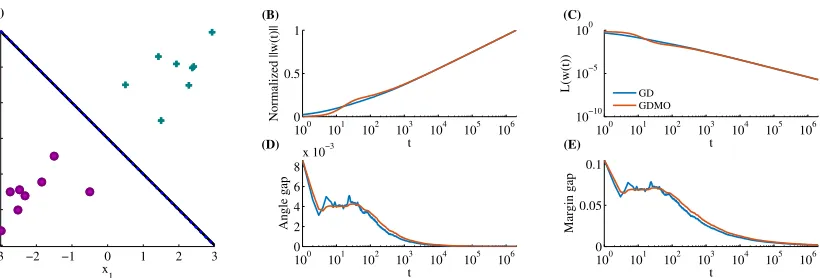
A numerical illustration of the convergence is depicted in Figure 1. As predicted by the theory, the norm kw(t)k grows logarithmically (note the semi-log scaling), and w(t) converges to the max-margin separator, but only logarithmically, while the loss itself decreases very rapidly (note the log-log scaling).
An important practical consequence of our theory, is that although the margin ofw(t)keeps improving, and so we can expect the population (or test) misclassification error ofw(t)to improve for many datasets, the same cannot be said about the expected population loss (or test loss)! At the limit, the direction ofw(t)will converge toward the max margin predictorw. Althoughˆ wˆ has zero training error, it will not generally have zero misclassification error on the population, or on a test or a validation set. Since the norm ofw(t)will increase, if we use the logistic loss or any other convex loss, the loss incurred on those misclassified points will also increase. More formally, consider the logistic loss`(u) = log(1+e−u)and define also the hinge-at-zero lossh(u) = max(0,−u). Sincewˆ classifies all training points correctly, we have that on the training setPN
n=1h( ˆw>xn) = 0. However,
on the population we would expect some errors and soE[h( ˆw>x)]>0. Sincew(t)≈wˆlogtand
`(αu)→αh(u)asα→ ∞, we have:
E[`(w(t)>x)]≈E[`((logt) ˆw>x)]≈(logt)E[h( ˆw>x)] = Ω(logt). (12)
That is, the population loss increases logarithmically while the margin and the population misclassifi-cation error improve. Roughly speaking, the improvement in misclassifimisclassifi-cation does not out-weight the increase in the loss of those points still misclassified.
The increase in the test loss is practically important because the loss on a validation set is frequently used to monitor progress and decide on stopping. Similar to the population loss, the validation loss will increase logarithmically witht, if there is at least one sample in the validation set which is classified incorrectly by the max margin vector (since we would not expect zero validation error). More precisely, as a direct consequence of Theorem 3 (as shown on Appendix D):
Corollary 6 Let`be the logistic loss, andV be an independent validation set, for which∃x∈ V
such thatx>wˆ <0. Then the validation loss increases as
Lval(w(t)) =X x∈V
`w(t)>x= Ω(log(t)).
100 101 102 103 104 105 106 0
0.5 1
Normalized ||w(t)||
t
(B)
100 101 102 103 104 105 106
10−10
10−5
100
L(w(t))
t
(C)
100 101 102 103 104 105 106
0 2 4 6 8
x 10−3
Angle gap
t
(D)
100 101 102 103 104 105 106
0 0.05 0.1
Margin gap
t
(E)
−3 −2 −1 0 1 2 3
−3 −2 −1 0 1 2 3
x
1
x2
(A)
GD GDMO
Figure 1: Visualization of or main results on a synthetic dataset in which theL2max margin vector ˆ
wis precisely known. (A)The dataset (positive and negatives samples (y = ±1) are respectively denoted by0+0and0◦0), max margin separating hyperplane (black line), and the asymptotic solution of GD (dashed blue). For both GD and GD with momentum (GDMO), we show:(B)The norm ofw(t), normalized so it would equal to1at the last iteration, to facilitate comparison. As expected (eq. 3), the norm increases logarithmically; (C)the training loss. As expected, it decreases as t−1 (eq. 11); and(D&E)the angle and margin gap ofw(t)fromwˆ (eqs. 9 and 10). As expected, these are logarithmically decreasing to zero.Implementation details:The dataset includes four support vectors: x1 = (0.5,1.5),x2 = (1.5,0.5)withy1 = y2 = 1, andx3 = −x1, x4 = −x2 with
y3 = y4 = −1 (the L2 normalized max margin vector is thenwˆ = (1,1)/
√ 2 with margin equal to√2), and12other random datapoints (6from each class), that are not on the margin. We used a learning rateη = 1/σmax2 (X), whereσmax2 (X)is the maximal singular value ofX, momentumγ = 0.9for GDMO, and initialized at the origin.
kw(t)kgetting larger, and in fact the model might be getting better (increasing the margin and possibly decreasing the error rate).
4. Extensions
4.1. Multi-Class Classification with Cross-Entropy Loss
So far, we have discussed the problem of binary classification, but in many practical situations we have more then two classes. For multi-class problems, the labels are the class indices yn ∈
[K], {1, . . . , K}and we learn a predictorwkfor each classk∈ [K]. A common loss function
in multi-class classification is the following cross-entropy loss with a softmax output, which is a generalization of the logistic loss:
L {wk}k∈[K]
=−
N X
n=1
log exp w
> ynxn
PK
k=1exp w>kxn
!
(13)
What do the linear predictorswk(t)converge to if we minimize the cross-entropy loss by gradient
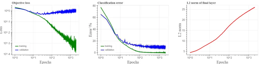
Figure 2: Training of a convolutional neural network on CIFAR10 using stochastic gradient descent with constant learning rate and momentum, softmax output and a cross entropy loss, where we achieve8.3%final validation error. We observe that, approximately: (1) The training loss decays as at−1, (2) theL2norm of last weight layer increases logarithmically, (3) after a while, the validation loss starts to increase, and (4) in contrast, the validation (classification) error slowly improves.
again, the predictors diverge to infinity and the loss converges to zero. Furthermore, we prove the following Theorem:
Theorem 7 For almost all multiclass datasets (i.e., except for a measure zero) which are linearly separable (i.e. the constraints in eq. 15 below are feasible), any starting pointw(0)and any small enough stepsize, the iterates of gradient descent on 13 will behave as:
wk(t) = ˆwklog(t) +ρk(t), (14)
where the residualρk(t)is bounded andwˆkis the solution of the K-class SVM:
argminw1,...,wk
K X
k=1
||wk||2s.t.∀n,∀k=6 yn:w>ynxn≥w
>
kxn+ 1. (15)
4.2. Deep networks
So far we have only considered linear prediction. Naturally, it is desirable to generalize our results also to non-linear models and especially multi-layer neural networks.
Even without a formal extension and description of the precise bias, our results already shed light on how minimizing the cross-entropy loss with gradient descent can have a margin maximizing effect, how the margin might improve only logarithmically slow, and why it might continue to improve even as the validation loss increases. These effects are demonstrated in Figure 2 and Table 1 which portray typical training of a convolutional neural network using unregularized gradient descent4. As can be seen, the norm of the weight increases, but the validation error continues decreasing, albeit very slowly (as predicted by the theory), even after the training error is zero and the training loss is extremely small. We can now understand how even though the loss is already extremely small, some sort of margin might be gradually improving as we continue optimizing. We can also observe how the validation loss increases despite the validation error decreasing, as discussed in Section 3.
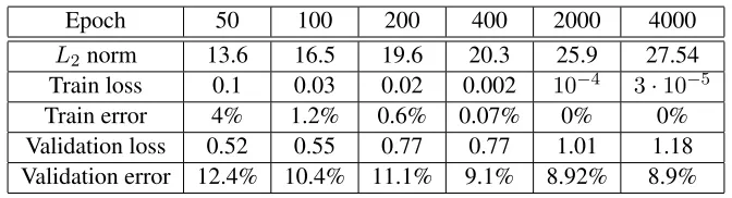
Epoch 50 100 200 400 2000 4000
L2norm 13.6 16.5 19.6 20.3 25.9 27.54 Train loss 0.1 0.03 0.02 0.002 10−4 3·10−5 Train error 4% 1.2% 0.6% 0.07% 0% 0% Validation loss 0.52 0.55 0.77 0.77 1.01 1.18 Validation error 12.4% 10.4% 11.1% 9.1% 8.92% 8.9%
Table 1: Sample values from various epochs in the experiment depicted in Fig. 2.
As an initial advance toward tackling deep network, we can point out that for several special cases, our results may be directly applied to multi-layered networks. First, somewhat trivially, our results may be applied directly to the last weight layer of a neural network if the last hidden layer becomes fixed and linearly separable after a certain number of iterations. This can become true, either approximately, if the input to the last hidden layer is normalized (e.g., using batch norm), or exactly, if the last hidden layer is quantized (Hubara et al., 2018).
Second, as we show next, our results may be applied exactly on deep networks if only a single weight layer is being optimized, and, furthermore, after a sufficient number of iterations, the activation units stop switching and the training error goes to zero.
Corollary 8 We examine a multilayer neural network with component-wise ReLU functionsf(z) = max [z,0], and weights{Wl}Ll=1. Given inputxnand targetyn ∈ {−1,1}, the DNN produces a scalar output
un=WLf(WL−1f(· · ·W2f(W1xn))) and has loss`(ynun), where`obeys assumptions 2 and 3.
If we optimize a single weight layerwl= vec W>l
using gradient descent, so thatL(wl) =
PN
n=1`(ynun(wl))converges to zero, and∃t0 such that∀t > t0 the ReLU inputs do not switch
signs, thenwl(t)/kwl(t)kconverges to
ˆ
wl= argmin
wl
kwlk2 s.t. ynun(wl)≥1.
ProofWe examine the output of the network given a single inputxn, fort > t0. Since the ReLU inputs do not switch signs, we can writevl, the output of layerl, as
vl,n= l Y
m=1
Am,nWmxn,
where we definedAl,nforl < Las a diagonal 0-1 matrix, which diagonal is the ReLU slopes at
layerl, samplen, andAL,n= 1. Additionally, we define
δl,n=Al,n l+1
Y
m=L
Wm>Am,n; ˜xl,n=δl,n⊗ul−1,n.
Using this notation we can write
un(wl) =vL,n= L Y
m=1
100 101 102 103 104 105 106 0
0.5 1
Normalized ||w(t)||
t
(B)
100 101 102 103 104 105 106 10−20
10−10 100
L(w(t))
t
(C)
GD GDMO ADAM
100 101 102 103 104 105 106 0
0.05 0.1 0.15
Angle gap
t
(D)
100 101 102 103 104 105 106 0
1 2
Margin gap
t
(E)
−50 0 50
−50 0 50
x1
x2 (A)
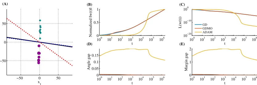
Figure 3: Same as Fig. 1, except we multiplied allx2 values in the dastaset by20, and also train using ADAM. The final weight vector produced after2·106 epochs of optimization using ADAM (red dashed line) does not converge to L2 max margin solution (black line), in contrast to GD (blue dashed line), or GDMO.
This implies that
L(wl) = N X
n=1
`(ynun(wl)) = N X
n=1
`ynx˜>l,nwl
,
which is the same as the original linear problem. Since the loss converges to zero, the dataset {x˜l,n, yn}Nn=1must be linearly separable. Applying Theorem 3, and recalling thatu(wl) = ˜x>l wl
from eq. 16, we prove this corollary.
Importantly, this case is non-convex, unless we are optimizing the last layer. Note we assumed ReLU functions for simplicity, but this proof can be easily generalized for any other piecewise linear constant activation functions (e.g., leaky ReLU, max-pooling).
Lastly, in a follow-up work (Gunasekar et al., 2018b), given a few additional assumptions, extended our results to linear predictors which can be written as a homogeneous polynomial in the parameters. These results seem to indicate that, in many cases, GD operating on exp-tailed loss with positively homogeneous predictors aims to a specific direction. This is the direction of the max margin predictor minimizing theL2 norm in the parameter space. It is not yet clear how to generally translate such an implicit bias in the parameter space to the implicit bias in the predictor space — except in special cases, such as deep linear neural nets, as we have shown in (Gunasekar et al., 2018b). Moreover, in non-linear neural nets, there are many equivalent max-margin solutions which minimize theL2norm of the parameters. Therefore, it is natural to expect that GD would have additional implicit biases, which select a specific subset of these solutions.
4.3. Other optimization methods
and constructing learning methods attuned to the inductive biases we expect. Can we characterize the implicit bias and convergence rate in other optimization methods?
In Figure 1 we see that adding momentum does not qualitatively affect the bias induced by gradient descent. In Figure 4 in Appendix F we also repeat the experiment using stochastic gradient descent, and observe a similar asymptotic bias (this was later proved in Nacson et al. (2018)). This is consistent with the fact that momentum, acceleration and stochasticity do not change the bias when using gradient descent to optimize an under determined least squares problem. It would be beneficial, though, to rigorously understand how much we can generalize our result to gradient descent variants, and how the convergence rates might change in these cases.
On the other hand, as an example of how changing the optimization algorithm does change the bias, consider adaptive methods, such as AdaGrad (Duchi et al., 2011) and ADAM (Kingma and Ba, 2015). In Figure 3 we show the predictors obtained by ADAM and by gradient descent on a simple data set. Both methods converge to zero training error solutions. But although gradient descent converges to theL2max margin predictor, as predicted by our theory, ADAM does not. The implicit bias of adaptive methods has in fact been a recent topic of interest, with Hoffer et al. (2017) and Wilson et al. (2017) suggesting they lead to worse generalization, and Wilson et al. (2017) providing examples of the differences in the bias for linear regression problems with the squared loss. Can we characterize the bias of adaptive methods for logistic regression problems? Can we characterize the bias of other optimization methods, providing a general understanding linking optimization algorithms with their biases?
In a follow-up paper (Gunasekar et al., 2018) provided initial answers to these questions. Gu-nasekar et al. (2018) derived a precise characterization of the limit direction of steepest descent for general norms when optimizing the exp-loss, and show that for adaptive methods such as Adagrad the limit direction can depend on the initial point and step size and is thus not as predictable and robust as with non-adaptive methods.
4.4. Other loss functions
In this work we focused on loss functions with exponential tail and observed a very slow, logarithmic convergence of the normalized weight vector to theL2max margin direction. A natural question that follows is how does this behavior change with types of loss function tails. Specifically, does the normalized weight vector always converge to theL2max margin solution? How is the convergence rate affected? Can we improve the convergence rate beyond the logarithmic rate found in this work? In a follow-up work Nacson et al. (2018) provided partial answers to these questions. They proved that the exponential tail has the optimal convergence rate, for tails for which`0(u) is of the formexp(−uν) withν > 0.25. They then conjectured, based on heuristic analysis, that the exponential tail is optimal among all possible tails. Furthermore, they demonstrated that polynomial or heavier tails do not converge to the max margin solution. Lastly, for the exponential loss they proposed a normalized gradient scheme which can significantly improve convergence rate, achieving
O(log(t)/√t).
4.5. Matrix Factorization
matrix factorization can be viewed as a two-layer network with linear activations, this is perhaps the simplest deep model one can study in full, and can thus provide insight and direction to studying more complex neural networks. Gunasekar et al. conjectured, and provided theoretical and empirical evidence, that gradient descent on the factorization for an under-determined problem converges to the minimum nuclear norm solution, but only if the initialization is infinitesimally close to zero and the step-sizes are infinitesimally small. With finite step-sizes or finite initialization, Gunasekar et al. could not characterize the bias.
The follow-up paper (Gunasekar et al., 2018) studied this same problem with exponential loss instead of squared loss. Under additional assumptions on the asymptotic convergence of update directions and gradient directions, they were able to relate the direction of gradient descent iterates on the factorized parameterization asymptotically to the maximum margin solution with unit nuclear norm. Unlike the case of squared loss, the result for exponential loss are independent of initialization and with only mild conditions on the step size. Here again, we see the asymptotic nature of exponential loss on separable data nullifying the initialization effects thereby making the analysis simpler compared to squared loss.
5. Summary
We characterized the implicit bias induced by gradient descent on homogeneous linear predictors when minimizing smooth monotone loss functions with an exponential tail. This is the type of loss commonly being minimized in deep learning. We can now rigorously understand:
1. How gradient descent, without early stopping, induces implicitL2regularization and converges to the maximumL2margin solution, when minimizing for binary classification with logistic loss, exp-loss, or other exponential tailed monotone decreasing loss, as well as for multi-class classification with cross-entropy loss. Notably, even though the logistic loss and the exp-loss behave very different on non-separable problems, they exhibit the same behaviour for separable problems. This implies that the non-tail part does not affect the bias. The bias is also independent of the step-size used (as long as it is small enough to ensure convergence) and is also independent on the initialization (unlike for least square problems).
2. The convergence of the direction of gradient descent updates to the maximum L2 margin solution, however is very slow compared to the convergence of training loss, which explains why it is worthwhile continuing to optimize long after we have zero training error, and even when the loss itself is already extremely small.
3. We should not rely on plateauing of the training loss or on the loss (logistic or exp or cross-entropy) evaluated on a validation data, as measures to decide when to stop. Instead, we should look at the0–1error on the validation dataset. We might improve the validation and test errors even when when the decrease in the training loss is tiny and even when the validation loss itself increases.
importantly, we hope that our analysis can open the door to further analysis of different optimization methods or in different models, including deep networks, where implicit regularization is not well understood even for least square problems, or where we do not have such a natural guess as for gradient descent on linear problems. Analyzing gradient descent on logistic/cross-entropy loss is not only arguably more relevant than the least square loss, but might also be technically easier.
Acknowledgments
Appendix
Appendix A. Proof of Theorems 3 and 4 for almost every dataset
In the following sub-sections we first prove Theorem 9 below, which is a version of Theorem 3, specialized for almost every dataset. We then prove Theorem 4 (which is already stated for almost every dataset).
Theorem 9 For almost every dataset which is linearly separable (Assumption 1), anyβ-smooth decreasing loss function (Assumption 2) with an exponential tail (Assumption 3), any stepsize η < 2β−1σmax−2 (X)and any starting pointw(0), the gradient descent iterates (as in eq. 2) will behave as:
w(t) = ˆwlogt+ρ(t) , (17)
wherewˆ is theL2max margin vector
ˆ
w= argmin w∈Rd
kwk2 s.t.∀n: w>xn≥1,
the residualρ(t)is bounded, and so
lim
t→∞
w(t) kw(t)k =
ˆ w kwˆk. In the following proofs, for any solutionw(t), we define
r(t) =w(t)−wˆlogt−w˜,
wherewˆ andw˜ follow the conditions of Theorems 3 and 4,i.e. wˆ is theL2is the max margin vector defined above, andw˜ is a vector which satisfies eq. 7:
∀n∈ S : ηexp−x>nw˜=αn, (18)
where we recall that we denotedXS ∈Rd×|S|as the matrix whose columns are the support vectors,
a subsetS ⊂ {1, . . . , N}of the columns ofX= [x1, . . . ,xN]∈Rd×N.
In Lemma 12 (Appendix B) we prove that for almost every datasetαis uniquely defined, there are no more thendsupport vectors andαn6= 0,∀n∈ S. Therefore, eq. 18 is well-defined in those
cases. If the support vectors do not span the data, then the solutionw˜ to eq. 18 might not be unique. In this case, we can use any such solution in the proof.
We furthermore denote the minimum margin to a non-support vector as:
θ= min
n /∈Sx >
nwˆ >1, (19)
and byCi,i,ti (i ∈ N) various positive constants which are independent oft. Lastly, we define
P1 ∈Rd×das the orthogonal projection matrix5to the subspace spanned by the support vectors (the
columns ofXS), andP¯1 =I−P1as the complementary projection (to the left nullspace ofXS).
5. This matrix can be written asP1=XSX+S, whereM †
A.1. Simple proof of Theorem 9
In this section we first examine the special case that`(u) =e−uand take the continuous time limit of gradient descent:η→0, so
˙
w(t) =−∇L(w(t)).
The proof in this case is rather short and self-contained (i.e., does not rely on any previous results), and so it helps to clarify the main ideas of the general (more complicated) proof which we will give in the next sections.
Recall we defined
r(t) =w(t)−log (t) ˆw−w˜ . (20) Our goal is to show thatkr(t)kis bounded, and thereforeρ(t) = r(t) + ˜wis bounded. Eq. 20 implies that
˙
r(t) = ˙w(t)−1
twˆ =−∇L(w(t))−
1
twˆ (21)
and therefore
1 2
d
dtkr(t)k
2 = ˙r>(t)r(t)
=
N X
n=1 exp
−x>nw(t)
x>nr(t)−1 twˆ
>
r(t)
=
" X
n∈S
exp−log (t) ˆw>xn−w˜>xn−x>nr(t)
x>nr(t)− 1 twˆ
>r(t)
#
+
X
n6∈S/
exp−log (t) ˆw>xn−w˜>xn−x>nr(t)
x>nr(t)
, (22)
where in the last equality we used eq. 20 and decomposed the sum over support vectors S and non-support vectors. We examine both bracketed terms. Recall thatwˆ>xn= 1forn∈ S, and that
we defined (in eq. 18)w˜ so thatP
n∈Sexp −w˜>xn
xn= ˆw. Thus, the first bracketed term in eq.
22 can be written as
1
t
X
n∈S
exp
−w˜>xn−x>nr(t)
x>nr(t)−1 t
X
n∈S
exp
−w˜>xn
x>nr(t)
=1
t
X
n∈S
exp−w˜>xn exp
−x>nr(t)−1x>nr(t)≤0, (23)
since∀z, z(e−z−1)≤ 0. Furthermore, since∀z e−zz ≤1andθ = argminn /∈Sx>nwˆ >1(eq.
19), the second bracketed term in eq. 22 can be upper bounded by
X
n6∈S/
exp
−log (t) ˆw>xn−w˜>xn
exp
−x>nr(t)
x>nr(t)≤ 1 tθ
X
n6∈S/
exp
−w˜>xn
. (24)
Substituting eq. 23 and 24 into eq. 22 and integrating, we obtain, that∃C, C0such that
∀t1,∀t > t1 :kr(t)k2− ||r(t1)||2 ≤C
Z t
t1
dt tθ ≤C
sinceθ >1(eq. 19). Thus, we showed thatr(t)is bounded, which completes the proof for the special case.
A.2. Complete proof of Theorem 9
Next, we give the proof for the general case (non-infinitesimal step size, and exponentially-tailed functions). Though it is based on a similar analysis as in the special case we examined in the previous section, it is somewhat more involved since we have to bound additional terms.
First, we state two auxiliary lemmata, that are proven below in appendix sections A.4 and A.5:
Lemma 10 LetL(w)be aβ-smooth non-negative objective. Ifη <2β−1, then, for anyw(0), with the GD sequence
w(t+ 1) =w(t)−η∇L(w(t)) (25)
we have thatP∞
u=0k∇L(w(u))k
2<∞
and thereforelimt→∞k∇L(w(t))k2= 0.
Lemma 11 We have
∃C1, t1 : ∀t > t1 : (r(t+ 1)−r(t))>r(t)≤C1t−min(θ,1+1.5µ+,1+0.5µ−). (26)
Additionally,∀1 >0,∃C2, t2, such that∀t > t2, if
kP1r(t)k ≥1, (27)
then the following improved bound holds
(r(t+ 1)−r(t))>r(t)≤ −C2t−1 <0. (28) Our goal is to show thatkr(t)kis bounded, and thereforeρ(t) =r(t) + ˜wis bounded. To show this, we will upper bound the following equation
kr(t+ 1)k2 =kr(t+ 1)−r(t)k2+ 2 (r(t+ 1)−r(t))>r(t) +kr(t)k2 (29) First, we note that first term in this equation can be upper-bounded by
kr(t+ 1)−r(t)k2
(1)
= kw(t+ 1)−wˆlog (t+ 1)−w˜ −w(t) + ˆwlog (t) + ˜wk2
(2)
= k−η∇L(w(t))−wˆ [log (t+ 1)−log (t)]k2 =η2k∇L(w(t))k2+kwˆk2log2 1 +t−1
+ 2ηwˆ>∇L(w(t)) log 1 +t−1
(3)
≤ η2k∇L(w(t))k2+kwˆk2t−2 (30)
where in(1)we used eq. 20, in(2)we used eq. 2, and in(3)we used∀x >0 : x≥log (1 +x)>0, and also that
ˆ
w>∇L(w(t)) =
N X
n=1
`0w(t)>xn
ˆ
sincewˆ>xn≥1(from the definition ofw) andˆ `0(u)≤0.
Also, from Lemma 10 we know that
k∇L(w(t))k2=o(1) and
∞
X
t=0
k∇L(w(t))k2<∞. (32)
Substituting eq. 32 into eq. 30, and recalling that at−ν power series converges for anyν >1, we can findC0such that
kr(t+ 1)−r(t)k2 =o(1) and
∞
X
t=0
kr(t+ 1)−r(t)k2 =C0 <∞. (33)
Note that this equation also implies that∀0
∃t0 :∀t > t0 :|kr(t+ 1)k − kr(t)k|< 0. (34) Next, we would like to bound the second term in eq. 29. From eq. 26 in Lemma 11, we can find
t1, C1such that∀t > t1:
(r(t+ 1)−r(t))>r(t)≤C1t−min(θ,1+1.5µ+,1+0.5µ−). (35) Thus, by combining eqs. 35 and 33 into eq. 29, we find
kr(t)k2− kr(t1)k2
=
t−1
X
u=t1 h
kr(u+ 1)k2− kr(u)k2i
≤C0+ 2
t−1
X
u=t1
C1u−min(θ,1+1.5µ+,1+0.5µ−)
which is a bounded, since θ > 1(eq. 19) and µ−, µ+ > 0(Definition 2). Therefore,kr(t)kis bounded.
A.3. Proof of Theorem 4
All that remains now is to show thatkr(t)k →0ifrank (XS) = rank (X), and thatw˜ is unique
givenw(0). To do so, this proof will continue where the proof of Theorem 3 stopped, using notations and equations from that proof.
Sincer(t)has a bounded norm, its two orthogonal componentsr(t) =P1r(t) + ¯P1r(t)also have bounded norms (recall thatP1,P¯1were defined in the beginning of appendix section A). From eq. 2,∇L(w)is spanned by the columns ofX. Ifrank (XS) = rank (X), then it is also spanned
by the columns ofXS, and soP¯1∇L(w) = 0. Therefore,P¯1r(t)is not updated during GD, and remains constant. Sincew˜ in eq. 20 is also bounded, we can absorb this constantP¯1r(t)intow˜ without affecting eq. 7 (since∀n∈ S : x>nP¯1r(t) = 0). Thus, without loss of generality, we can assume thatr(t) =P1r(t).
We define the set
By contradiction, we assume that the complementary set is not finite,
¯
T ={t >max [t2, t0] :kr(t)k ≥1} .
Additionally, the set T is not finite: if it were finite, it would have had a finite maximal point
tmax∈ T, and then, combining eqs. 28, 29, and 33, we would find that∀t > tmax
kr(t)k2− kr(tmax)k2 =
t−1
X
u=tmax h
kr(u+ 1)k2− kr(u)k2i≤C0−2C2
t−1
X
u=tmax
u−1 → −∞,
which is impossible sincekr(t)k2≥0. Furthermore, eq. 33 implies that
t X
u=0
kr(u+ 1)−r(t)k2 =C0−h(t)
whereh(t)is a positive monotone function decreasing to zero. Lett3, tbe any two points such that
t3 < t,{t3, t3+ 1, . . . t} ⊂T¯, and(t3−1)∈ T. For all sucht3andt, we have
kr(t)k2 ≤ kr(t3)k2+
t−1
X
u=t3 h
kr(u+ 1)k2− kr(u)k2i
=kr(t3)k2+
t−1
X
u=t3 h
kr(u+ 1)−r(u)k2+ 2 (r(u+ 1)−r(u))>r(u)i
≤ kr(t3)k2+h(t3)−h(t−1)−2C2
t−1
X
u=t3
u−1
≤ kr(t3)k2+h(t3). (36)
Also, recall that t3 > t0, so from eq. 34, we have that |kr(t3)k − kr(t3−1)k| < 0. Since
kr(t3−1)k< 1(fromT definition), we conclude thatkr(t3)k ≤1+0. Moreover, sinceT¯ is an infinite set, we can chooset3as large as we want. This implies that∀2 >0we can findt3such that
2> h(t3), sinceh(t)is a monotonically decreasing function. Therefore, from eq. 36,∀1, 0, 2,
∃t3 ∈T¯ such that
∀t > t3 : kr(t)k2 ≤1+0+2. This implies thatkr(t)k →0.
Lastly, we note that sinceP¯1r(t)is not updated during GD, we have thatP¯1( ˜w−w(0)) = 0. This setsw˜ uniquely, together with eq. 7.
A.4. Proof of Lemma 10
Lemma 10 LetL(w)be aβ-smooth non-negative objective. Ifη <2β−1, then, for anyw(0), with the GD sequence
w(t+ 1) =w(t)−η∇L(w(t)) (25)
we have thatP∞
u=0k∇L(w(u))k
2
This proof is a slightly modified version of the proof of Theorem 2 in (Ganti, 2015). Recall a well-known property ofβ-smooth functions:
f(x)−f(y)− ∇f(y)
>
(x−y)
≤
β
2 kx−yk 2 .
(37)
From theβ-smoothness ofL(w)
L(w(t+ 1))≤ L(w(t)) +∇L(w(t))>(w(t+ 1)−w(t)) + β
2kw(t+ 1)−w(t)k 2
=L(w(t))−ηk∇L(w(t))k2+βη 2
2 k∇L(w(t))k 2
=L(w(t))−η
1−βη 2
k∇L(w(t))k2
Thus, we have
L(w(t))− L(w(t+ 1))
η
1−βη2
≥ k∇L(w(t))k2
which implies
t X
u=0
k∇L(w(u))k2 ≤
t X
u=0
L(w(u))− L(w(u+ 1))
η
1− βη2
= L(w(0))− L(w(t+ 1))
η
1− βη2
.
The right hand side is upper bounded by a finite constant, sinceL(w(0))<∞and0≤ L(w(t+ 1)). This implies
∞
X
u=0
k∇L(w(u))k2<∞,
and thereforek∇L(w(t))k2→0.
A.5. Proof of Lemma 11
Recall that we definedr(t) = w(t)−wˆ logt−w, with˜ wˆ andw˜ follow the conditions of the Theorems 3 and 4,i.e,wˆ is theL2max margin vector and (eq. 4), and eq. 7 holds
∀n∈ S : ηexp
−x>nw˜
=αn.
Lemma 11 We have
∃C1, t1 : ∀t > t1 : (r(t+ 1)−r(t))>r(t)≤C1t−min(θ,1+1.5µ+,1+0.5µ−). (26)
Additionally,∀1 >0,∃C2, t2, such that∀t > t2, if
kP1r(t)k ≥1, (27)
then the following improved bound holds
From Lemma 1, ∀n : limt→∞w(t)>xn =∞. In addition, from assumption 3 the negative
loss derivative−`0(u) has an exponential taile−u (recall we assumea = c = 1without loss of generality). Combining both facts, we have positive constantsµ−, µ+,t−andt+such that∀n
∀t > t+:−`0
w(t)>xn
≤1 + exp−µ+w(t)>xn
exp−w(t)>xn
(38)
∀t > t−:−`0
w(t)>xn
≥1−exp−µ−w(t)>xn
exp−w(t)>xn
(39)
Next, we examine the expression we wish to bound, recalling thatr(t) =w(t)−wˆ logt−w:˜ (r(t+ 1)−r(t))>r(t)
= (−η∇L(w(t))−wˆ [log (t+ 1)−log (t)])>r(t)
=−η
N X
n=1
`0w(t)>xn
x>nr(t)−wˆ>r(t) log 1 +t−1
= ˆw>r(t)
t−1−log 1 +t−1
−ηX
n /∈S
`0w(t)>xn
x>nr(t) (40)
−ηX
n∈S
h
t−1exp−w˜>xn
+`0w(t)>xn i
x>nr(t)
where in last line we used eqs. 6 and 7 to obtain
ˆ w=X
n∈S
αnxn=η X
n∈S
exp−w˜>xn
xn.
We examine the three terms in eq. 40. The first term can be upper bounded by
ˆ
w>r(t)
t−1−log 1 +t−1
≤maxhwˆ>r(t),0i
t−1−log 1 +t−1
(1)
≤max
h
ˆ
w>P1r(t),0
i
t−2
(2)
≤
(
kwˆk1t−2 ,if kP1r(t)k ≤1
o t−1 ,if kP1r(t)k> 1
(41)
where in(1)we used thatP¯1wˆ = ¯P1XSα= 0from eq. 6, and in(2)we used thatwˆ>r(t) =o(t),
since
ˆ
w>r(t) = ˆw> w(0)−η
t X
u=0
∇L(w(u))−wˆ log (t)−w˜
!
≤wˆ>(w(0)−w˜ −wˆ log (t))−ηt min 0≤u≤twˆ
>∇L
(w(u)) =o(t)
where in the last line we used that∇L(w(t)) =o(1), from Lemma 10.
Next, we upper bound the second term in eq. 40. From eq. 38∃t0+, such that∀> t0 > t0+,
Therefore,∀t > t0+:
−ηX
n /∈S `0
w(t)>xn
x>nr(t)
≤ −η X
n /∈S:x> nr(t)≥0
`0w(t)>xn
x>nr(t)
(1)
≤η X
n /∈S:x> nr(t)≥0
2 exp−w(t)>xn
x>nr(t)
(2)
≤η X
n /∈S:x> nr(t)≥0
2t−x>nwˆ exp
−w˜>xn−x>nr(t)
x>nr(t)
(3)
≤η X
n /∈S:x> nr(t)≥0
2t−x>nwˆ exp
−w˜>xn
(4)
≤ηNexp
−min
n w˜
>
xn
t−θ (43)
where in (1) we used eq. 42, in(2) we usedw(t) = ˆwlogt+ ˜w+r(t), in (3)we used
xe−x≤1andx>nr(t)≥0,and in(4)we usedθ >1, from eq. 19. Lastly, we will bound the sum in the third term in eq. 40
−ηX
n∈S
h
t−1exp−w˜>xn
+`0w(t)>xn i
x>nr(t) . (44)
We examine each termnin this sum, and divide into two cases, depending on the sign ofx>nr(t). First, ifx>nr(t)≥0, then termnin eq. 44 can be upper bounded∀t > t+, using eq. 38, by
ηt−1exp−w˜>xn h
1 +t−µ+exp−µ
+w˜>xn
exp−x>nr(t)−1ix>nr(t) (45) We further divide into cases:
1. Ifx>nr(t)
≤C0t−0.5µ+, then we can upper bound eq. 45 with
ηexp−(1 +µ+) min
n w˜
>x n
C0t−1−1.5µ+. (46)
2. Ifx>nr(t)
> C0t−0.5µ+, then we can findt00+> t0+to upper bound eq. 45∀t > t00+:
ηt−1e−w˜>xn
h
1 +t−µ+e−µ+w˜>xn
exp −C0t−0.5µ+
−1
i
x>nr(t) (1)
≤ηt−1e−w˜>xnh1 +t−µ+e−µ+w˜>xn 1−C
0t−0.5µ+ +C02t−µ+
−1ix>nr(t) ≤ηt−1e−w˜>xn
1−C0t−0.5µ+ +C02t−µ+
e−µ+minn w˜ >xn
t−µ+−C
0t−0.5µ+ +C02t−µ+
x>nr(t)
(2)
≤0,∀t > t00+ (47)
3. Ifx>nr(t)
≥2, then we definet000+ > t00+such thatt000+ >exp minnw˜>xn e0.52−1 −1/µ+
, and therefore∀t > t000+, we have 1 +t−µ+exp −µ
+w˜>xn
e−2 < e−0.52 .
This implies that∀t > t000+we can upper bound eq. 45 by −ηexp−max
n w˜
>x n
1−e−0.52
2t−1. (48)
Second, ifx>nr(t)<0, we again further divide into cases: 1. Ifx>nr(t)
≤C0t−0.5µ−, then, since−`0
w(t)>xn
>0, we can upper bound termnin eq. 44 with
ηt−1exp
−w˜>xn x
> nr(t)
≤ηexp
−min
n w˜
>
xn
C0t−1−0.5µ− (49)
2. Ifx>nr(t)
> C0t−0.5µ−, then, using eq. 39 we upper bound termnin eq. 44 with
ηh−t−1e−w˜>xn−`0w(t)>xn i
x>nr(t) ≤ηh−t−1e−w˜>xn+1−exp−µ−w(t)>xn
exp−w(t)>xn i
x>nr(t)
=ηt−1e−w˜>xnh1−exp−r(t)>xn 1− h
t−1e−w˜>xnexp−r(t)>xn
iµ−i
x
> nr(t)
(50)
Next, we will show that∃t0−> t−such that the last expression is strictly negative∀t > t0−.
LetM > 1be some arbitrary constant. Then, sinceht−1e−w˜>xnexp−r(t)>xn
iµ−
=
exp−µ−w(t)>xn
→0from Lemma 1,∃tM >max(t−, M e−w˜
>xn
)such that∀t > tM,
ifexp
−r(t)>xn
≥M >1then
exp−r(t)>xn 1− h
t−1e−w˜>xnexp−r(t)>xn
iµ−
≥M0 >1. (51)
Furthermore, if∃t > tM such thatexp
r(t)>xn
< M, then
exp−r(t)>xn 1− h
t−1e−w˜>xnexp−r(t)>xn
iµ−
>exp
−r(t)>xn 1− h
t−1e−w˜>xnM
iµ−
. (52)
which is lower bounded by
1 +C0t−0.5µ−
1−t−µ−he−w˜>xnMiµ− ≥1 +C0t−0.5µ−−t−µ−
h
e−w˜>xnM
iµ−
−t−1.5µ−he−w˜>xnMiµ−C
0
sincex>nr(t)
> C0t−0.5µ−,xn>r(t) <0andex ≥ 1 +x. In this case last line is strictly
larger than1for sufficiently larget. Therefore, after we substitute eqs. 51 and 52 into 50, we find that∃t0−> tM > t−such that∀t > t0−, termkin eq. 44 is strictly negative
η
h
−t−1e−w˜>xk−`0
w(t)>xk i
3. Ifx>kr(t)
≥2 , which is a special case of the previous case ( x>kr(t)
> C0t−0.5µ−) then
∀t > t0−, either eq. 51 or 52 holds. Furthermore, in this case,∃t00−> t0−andM00>1such that
∀t > t00−eq. 52 can be lower bounded by
exp (2)
1−ht−1e−w˜>xkM
iµ−
> M00 >1.
Substituting this, together with eq. 51, into eq. 50, we can findC00 >0such we can upper bound termkin eq. 44 with
−C00t−1,∀t > t00−. (54)
To conclude, we chooset0 = max
t000+, t00−
:
1. IfkP1r(t)k ≥1(as in Eq. 27), we have that
max
n∈S
x
> nr(t)
2 (1)
≥ 1
|S|
X
n∈S
x
> nP1r(t)
2 = 1
|S|
X
> SP1r(t)
2 (2)
≥ 1
|S|σ
2
min(XS)21 (55)
where in(1)we usedP>1xn = xn ∀n ∈ S, in(2)we denoted byσmin(XS), the minimal
non-zero singular value of XS and used eq. 27. Therefore, for some k,
x>kr
≥ 2 ,
q
|S|−1σ2min(XS)21. In this case, we denoteC000as the minimum betweenC00 (eq. 54) and
ηexp −maxnw˜>xn
1−e−0.52
2 (eq. 48). Then we find that eq. 44 can be upper bounded by−C000t−1+o t−1,∀t > t0, given eq. 27. Substituting this result, together with eqs. 41 and 43 into eq. 40, we obtain∀t > t0
(r(t+ 1)−r(t))>r(t)≤ −C000t−1+o t−1
.
This implies that∃C2 < C000and∃t2 > t0such that eq. 28 holds. This implies also that eq. 26 holds forkP1r(t)k ≥1.
2. Otherwise, ifkP1r(t)k< 1, we find that∀t > t0, each term in eq. 44 can be upper bounded by either zero (eqs. 47 and 53), or terms proportional tot−1−1.5µ+ (eq. 46) ort−1−0.5µ−, (eq. 49). Combining this together with eqs. 41, 43 into eq. 40 we obtain (for some positive constantsC3,C4,C5, andC6)
(r(t+ 1)−r(t))>r(t)≤C3t−1−1.5µ++C4t−1−0.5µ−+C5t−2+C6t−θ. Therefore,∃t1 > t0andC1such that eq. 26 holds.
Appendix B. Generic solutions of the KKT conditions in eq. 6
Lemma 12 For almost all datasets there is a uniqueαwhich satisfies the KKT conditions (eq. 6):
ˆ w=
N X
n=1
αnxn ∀n
αn≥0andwˆ>xn= 1
OR
αn= 0andwˆ>xn>1
For almost every setX, no more thandpointsxncan be on the same hyperplane. Therefore,
since all support vectors must lie on the same hyperplane, there can be at mostdsupport vectors, for almost everyX.
Given the set of support vectors,S, the KKT conditions of eq. 6 entail thatαn= 0ifn /∈ S and
1=X>Swˆ =X>SXSαS, (56)
where we denotedαS asα restricted to the support vector components. For almost every setX,
sinced≥ |S|,X>SXS∈R|S|×|S|is invertible. Therefore,αShas the unique solution
X>SXS
−1
1=αS. (57)
This implies that∀n ∈ S,αnis equal to a rational function in the components ofXS,i.e.,αn =
pn(XS)/qn(XS), wherepnandqnare polynomials in the components ofXS. Therefore, ifαn= 0,
thenpn(XS) = 0, so the components ofXSmust be at a root of the polynomialpn. The roots of the
polynomialpnhave measure zero, unless∀XS : pn(XS) = 0. However,pncannot be identically
equal to zero, since, for example, ifX>S =I|S|×|S|,0|S|×(d−|S|)
, thenX>SXS =I|S|×|S|, and so
in this case∀n∈ S,αn= 16= 0, from eq. 57.
Therefore, for a givenS, the event that "eq. 56 has a solution with a zero component" has a zero measure. Moreover, the union of these events, for all possibleS, also has zero measure, as a finite union of zero measures sets (there are only finitely many possible setsS ⊂ {1, . . . , N}). This implies that, for almost all datasetsX,αn = 0only ifn /∈ S. Furthermore, for almost all datasets
the solutionαis unique: for each dataset,Sis uniquely determined, and givenS , the solution eq. 56 is uniquely given by eq. 57.
Appendix C. Completing the proof of Theorem 3 for zero measure cases
In the preceding Appendices, we established Theorem 4, which only applied when all support vectors are associated with non-zero coefficients. This characterizes almost all data sets,i.e.all except for measure zero. We now turn to presenting and proving a more complete characterization of the limit behaviour of gradient descent, which covers all data sets, including those degenerate data sets not covered by Theorem 4, thus establishing Theorem 3.
In order to do so, we first have to introduce additional notation and a recursive treatment of the data set. We will define a sequence of data setsP¯mXS¯mobtained by considering only a subsetS¯m of the points, and projecting them using the projection matrixP¯m. We start, form = 0, with the
full original data set,i.e.S¯0 ={1, . . . , N}andP¯0=Id×d. We then definewˆmas the max margin
predictor forP¯m−1XS¯m−1,i.e.:
ˆ
wm= argmin
w∈Rd
kwk2 s.t.w>P¯m−1xn≥1∀n∈S¯m−1. (58)
In particular,wˆ1is the max margin predictor for the original data set. We then denoteSm+the indices
of non-support vectors for 58,Smthe indices of support vector of 58 with non-zero coefficients for
of support vector with zero coefficients. That is:
Sm+=nn∈S¯m−1|wˆm>P¯m−1xn>1 o
S=
m =
n
n∈S¯m−1|wˆm>P¯m−1xn= 1 o
= ¯Sm\ S+
m
Sm =
(
n∈ S=
m|∃α∈RN≥0 :wˆm = N X
k=1
αkP¯m−1xk, αn>0,∀i /∈ Sm=: αi = 0 )
¯
Sm =Sm=\ Sm. (59)
The problematic degenerate case, not covered by the analysis of Theorem 4, is when there are support vectors with zero coefficients,i.e., when S¯m 6= ∅. In this case we recurse on these
zero-coefficient support vectors (i.e., on S¯m), but only consider their components orthogonal to the
non-zero-coefficient support vectors (i.e., not spanned by points inSm). That is, we project using: ¯
Pm = ¯Pm−1
Id−XSmX
† Sm
(60)
where we denotedA†as the Moore-Penrose pseudo-inverse ofA. We also denotePm =Id−P¯m.
This recursive treatment continues as long asS¯m 6=∅, defining a sequencewˆmof max margin
predictors, for smaller and lower dimensional data setsP¯m−1XS¯m−1. We stop when
¯
Sm =∅and
denote the stopping stageM—that is,M is the minimalmsuch thatS¯m=∅. Our characterization
will be in terms of the sequencewˆ1, . . . ,wˆM. As established in Lemma 12 of Appendix B, for
almost all data sets we will not have support vectors with non-zero coefficients, and so we will have
M = 1, and so the characterization only depends on the max margin predictorwˆ1of the original data set. But, even for the measure zero of data sets in whichM >1, we provide the following more complete characterization:
Theorem 13 For all datasets which are linearly separable (Assumption 1) and given aβ-smooth loss function (Assumption 2) with an exponential tail (Assumption 3), gradient descent (as in eq. 2) with step sizeη <2β−1σmax−2 (X)and any starting pointw(0), the iterates of gradient descent can be written as:
w(t) =
M X
m=1 ˆ
wmlog◦m(t) +ρ(t), (61)
wherelog◦m(t) =
mtimes
z }| {
log log· · ·log (t),wˆm is theL2max margin vector defined in eq. 58, and the
residualρ(t)is bounded.
C.1. Auxiliary notation
We say that a functionf :N→Ris absolutely summable ifP∞t=1|f(t)|<∞, and then we denote
f(t)∈L1. Furthermore, we define
r(t) =w(t)−
M X
m=1
"
ˆ
wmlog◦m(t) + ˜wm+ m−1
X
k=1 ˇ wk,m
Qm−1
r=k log ◦r(t)
#
˜ w=
M X
m=1
˜ wm.
We define,∀m≥1,w˜mas the solution of
∀m≥1 :∀n∈ Sm: η X
n∈Sm
exp −
m X
k=1 ˜ w>kxn
!
¯
Pm−1xn= ˆwm, (62)
such that
Pm−1w˜m= 0 and ¯Pmw˜m = 0. (63)
The existence and uniqueness of the solution,w˜mare proved in appendix section C.4.
Lastly, we define,∀m > k≥1,wˇk,mas the solution of
X
n∈Sm
exp−w˜>xn
Pm−1xn= m−1
X
k=1
X
n∈Sk
exp−w˜>xn
xnx>n
wˇk,m (64)
such that
Pk−1wˇk,m= 0 andP¯kwˇk,m= 0. (65)
The existence and uniqueness of the solutionwˇk,mare proved in appendix section C.5.
Together, eqs. 62-65 entail the existence of a unique decomposition,∀m≥1 :
ˆ wm=η
X
n∈Sm
exp−w˜>xn
xn−η m−1
X
k=1
X
n∈Sk
exp−w˜>xn
xnx>n
wˇk,m (66)
given the constraints in eqs. 63 and 65 hold.
C.2. Proof of Theorem 13
In the following proofs, for any solutionw(t), we define
τ(t) =
M X
m=2 ˆ
wmlog◦m(t) + M X
m=1
m−1
X
k=1
ˇ wk,m
Qm−1
r=k log ◦r(t)
noting that
kτ(t+ 1)−τ(t)k ≤ Cτ tlog (t) and
r(t) =w(t)−wˆ1log (t)−w˜ −τ(t) (67) wherew˜ follow the conditions of Theorem 13. Our goal is to show thatkr(t)kis bounded. To show this, we will upper bound the following equation
First, we note that∃t0such that∀t > t0the first term in this equation can be upper bounded by
||r(t+ 1)−r(t)||2
(1)
= ||w(t+ 1)−wˆ1log (t+ 1)−τ(t+ 1)−w(t) + ˆw1log (t) +τ(t)||2 (2)
= || −η∇L(w(t))−wˆ1(log (t+ 1)−log (t))−(τ(t+ 1)−τ(t))||2 =η2||∇L(w(t))||2+kwˆ1k2log2 1 +t−1
+kτ(t+ 1)−τ(t)k2 + 2η∇L(w(t))> wˆ1log 1 +t−1
+τ(t+ 1)−τ(t)
+ 2 ˆw>1(τ(t+ 1)−τ(t)) log 1 +t−1
(3)
≤ η2||∇L(w(t))||2+kwˆ1k2t−2+Cτ2t−2log−2(t) + 2Cτkwˆ1kt−2log−1(t) ,∀t > t0 (69) where in (1) we used eq. 67, in (2) we used eq. 2 and in (3) we used∀x >0 : x≥log (1 +x)>0, and also using`0(w(t)>xn)<0for large enought, we have that
ˆ
w1log 1 +t−1+τ(t+ 1)−τ(t)
>
∇L(w(t))≤
N X
n=1
`0(w(t)>xn)
ˆ
w1>xnlog 1 +t−1−
kxnkCτ0
tlog (t)
(70) which is negative for sufficiently larget0(sincelog 1 +t−1
decreases ast−1, which is slower then 1/(tlog (t))),∀n: ˆw1>xn≥1and`0(u)≤0.
Also, from Lemma 10 we know that:
k∇L(w(t))k2 =o(1)and
∞
X
u=0
k∇L(w(u))k2 <∞ (71)
Substituting eq. 71 into eq. 69, and recalling thatt−ν1log−ν2(t)converges for anyν
1 >1and any
ν2, and so
κ0(t),||r(t+ 1)−r(t)||2 ∈L1. (72)
Also, in the next subsection we will prove that
Lemma 14 Letκ1(t)andκ2(t)be functions inL1, then
(r(t+ 1)−r(t))>r(t)≤κ1(t)kr(t)k+κ2(t) (73) Thus, by combining eqs. 73 and 72 into eq. 68, we find
kr(t+ 1)k2 ≤κ0(t) + 2κ1(t)kr(t)k+ 2κ2(t) +kr(t)k2
On this result we apply the following lemma (withφ(t) = kr(t)k,h(t) = 2κ1(t), andz(t) =
κ0(t) + 2κ2(t)), which we prove in appendix C.6:
Lemma 15 Letφ(t), h(t), z(t)be three functions fromNtoR≥0, andC1, C2, C3be three positive
constants. Then, ifP∞
t=1h(t)≤C1 <∞, and
φ2(t+ 1)≤z(t) +h(t)φ(t) +φ2(t) (74)
we have
φ2(t+ 1)≤C2+C3
t X
u=1
and obtain that
kr(t+ 1)k2≤C2+C3
t X
u=1
(κ0(u) + 2κ2(u))≤C4<∞,
since we assumed that∀i= 0,1,2 : κi(t)∈L1. This completes our proof.
C.3. Proof of Lemma 14
Before we prove Lemma 14, we prove the following auxilary Lemma:
Lemma 16 Consider the functionf(t) =t−ν1(log(t))−ν2(log log(t))−ν3. . .(log◦M(t))−νM+1. If
∃m0 ≤M + 1such thatνm0 >1and for allm 0< m
0,νm0 = 1, thenf(t)∈L1.
ProofTo prove Lemma 16, we will show that the improper integeralRt∞
1 f(t)dtfor anyt1 >0is
bounded,i.e.,∀t1 >0,
R∞
t1 f(t)dt < C. Using the integeral test for convergence (or Maclaurin–
Cauchy test) this in turn implies that∀t1 >0,P∞t1 f(t)< C, and thusf(t)∈L1.
First, ifm0 >1, thenν1 =ν2. . .=νm0−1 = 1andνm0 = 1 +for some >0. Using change
of variablesy = log◦(m0−1)(t), we have
dy= t
m0−2 Y
r=1
log◦r(t)
!−1
dt=t−ν1 m0−2
Y
r=1
(log◦r(t))−νr+1dt
and for allm > m0,
log◦(m−1)(t)
−νm
=
log◦(m−m0)(y)
−νm
≤(log(y))|νm|. Thus, denoting ˜
ν =PM+1
m=m0+1|νm|andlog
◦(m0−1)(t
1) =y1, we have
Z ∞
t1
f(t)dt=
Z ∞
y1
y−νm0
M+1
Y
m=m0+1
log◦m−m0(y)−νm
d(y)≤
Z ∞
y1
(log(y))ν˜
y1+ dy. (76)
For m0 = 1, we have ν1 = 1 +for some > 0, and for m > 1,
log◦(m−1)(t)
−νm
≤ (log(t))|νm|. Thus, denoting,ν˜=PM+1
m=2 |νm|, we have
R∞
t1 f(t)dt≤
R∞
t1
(log(t))ν˜
t1+ dt. Thus, for anym0, we only need to show that for allt1 >0, >0andν >˜ 0,
R∞
t1
(log(t))˜ν
t1+ dt <∞. Let us now look at Rt∞
1
(log(t))ν˜
t1+ dt. using u = (log(t))
˜
ν
and dv = t1+1, we have du = ˜
νt−1(log(t))ν˜−1andv=−t1. Using integration by parts,
R
udv=uv−R
vdu, we have
Z
(log(t))ν˜
t1+ dt=−
(log(t))˜ν
t +
¯
ν
Z
(log(t))ν˜−1