AUTUMN 2016, Vol II, No II, JOURNAL OF HYDRAULIC STRUCTURES Shahid Chamran University of Ahvaz
Journal of Hydraulic Structures J. Hydraul. Struct., 2016; 2(2):1-21
DOI: 10.22055/jhs.2016.12848
Groundwater Level Forecasting Using Wavelet and Kriging
Taher Rajaee1 Vahid Nourani 2 Fatemeh Pouraslan3
Abstract
In this research, a hybrid wavelet-artificial neural network (WANN) and a geostatistical method were proposed for spatiotemporal prediction of the groundwater level (GWL) for one month ahead. For this purpose, monthly observed time series of GWL were collected from September 2005 to April 2014 in 10 piezometers around Mashhad City in the Northeast of Iran. In temporal forecasting, an artificial neural network (ANN) and a WANN were trained for each piezometer. Kriging was used in spatial estimations. The comparison of the prediction accuracy of these two models illustrated that the WANN was more efficacious in prediction of GWL for one month ahead. Thereafter, in order to predict GWL in desired points in the study area, the kriging method was used and a Gaussian model was selected as the best variogram model. Ultimately, the WANN with coefficient of determination and root mean square error and mean absolute error, 0.836 and 0.335 and 0.273 respectively, in temporal forecasting and Gaussian model with root mean square, 0.253 as the best fitted model on Kriging method for spatial estimating were suitable choices for spatiotemporal GWL forecasting. The obtained map of groundwater level showed that the groundwater level was higher in the areas of plain located in mountainside areas. This fact can show that outcomes are respectively correct.
Keywords: Artificial neural network, wavelet, kriging, spatiotemporal prediction, groundwater level
Received: 15 September 2016; Accepted: 20 November 2016
1. Introduction
Most areas of the world are categorized as warm and arid areas; therefore, given the lack of precipitation and surface water, potable water and/or agricultural waters are only restricted to
1Associate Professor, Department of Civil Eng., University of Qom, Qom, Iran, E-mail addresses:
[email protected]; [email protected].
2 Professor, Department of Water Resources Engineering, Faculty of Civil Engineering, University of
Tabriz, Tabriz, Iran. E-mail addresses: [email protected].
3 M.Sc. in Hydraulic Structures, Department of Civil Eng., University of Qom, Qom, Iran, E-mail
AUTUMN 2016, Vol II, No II, JOURNAL OF HYDRAULIC STRUCTURES Shahid Chamran University of Ahvaz
groundwater resources. The prediction of GWL is a complex phenomenon and usually needs a lot of data and a long response time. Prediction of GWL is important for effective management of GWL such as aquifer development, contaminated remediation aquifer or performance assessment of planned water supply projects. Studies have been conducted to reduce the complexities of the problem in terms of developing practical techniques that do not require dwelling on algorithms and theories (Rajaee., 2011; Rajaee & Broumand, 2015; Ravansalar & Rajaee, 2015). Numerous studies with many methods and models for modelling of GWL have been reported, which are based on various theories (Yang et al., 2009; Shiri & Kisi, 2011; Yoon et al., 2011; Mohammadi, 2008; Nourani et al., 2011). One of these physical theories is based on numerical models that establish a governing equation simplifying the physics of flow in the subsurface and solve it with proper initial and boundary conditions (Yoon et al., 2011). This model requires various hydrological and geological patterns (Nakhaee & Saberinasr., 2012). The other models for prediction of GWL such as the Time Series model, the integrated time series model (Yang et al., 2009), autoregressive moving average model (Zhou et al., 2008; Kisi, 2010), the seasonal autoregressive moving average model (Gemitzi & Stefanopoulos, 2011; Zhou et al., 2008), the periodic autoregressive model, and the threshold autoregressive model (Wang et al., 2009) have been suggested in the past decades.
In the field of water resources and environmental engineering, artificial neural network (ANN) models have recently been applied to contamination modelling in shallow groundwaters (Sahoo et al., 2006), studying the ANN model for prediction of suspended sediment concentration (SSC) belonging to rivers (Rajaee et al., 2009) and forecasting the ozone episode days (Tsai et al., 2009). The ANN was used by Aziz & Wong (1992) to estimate aquifer parameters of groundwater. Lallahem et al (2005) used ANN to assess water tables in fractured media. Daliakopoulos et al (2005) investigated seven different types of network architectures and training algorithms for GWL forecasting in Messara valley with a neural network. The experiment results showed that a standard feed forward neural network trained with the Levenberg-Marquardt algorithm provided the best result. Nourani et al. (2008) evaluated the feasibility of using an ANN methodology for estimating the GWLs. The efficiency of the spatio-temporal ANN (STANN) model has beem compared with two hybrid neural-geostatistics (NG) and multivariate time series-geostatistics (TSG) models. The results showed that the ANNs provided the most accurate predictions in comparison with the other models. In a comparative assessment, Sahoo & Jha (2013) concluded that the ANN technique was superior to the multiple linear regression (MLR) technique in predicting the spatio-temporal distribution of the groundwater levels in a basin. In another research, Maiti & Tiwari (2014) compared the ANNs, the Bayesian neural networks and the adaptive neuro-fuzzy inference system (ANFIS) in GWL prediction. The results showed that the Bayesian neural networks (BNN) optimized by SCG models performed better than both the ANFIS and ANN optimized by a scaled conjugate gradient (SCG) (ANN.SCG).
If the input data are non-stationary, the accuracy of the neural networks decreases. One of the methods proposed to resolve this subject was wavelet analysis which has been applied to a number of problems in water resources and environmental engineering such as river flow modelling (Pasquini & Depetris, 2007). A non-stationary signal can be decomposed into a certain number of stationary signals by a wavelet transform. Then ANN is combined with the wavelet transform to improve the prediction accuracy (Zhou et al., 2008). Rajaee (2010) proposed a model by combining the wavelet analysis and neuro-fuzzy approach to predict the daily suspended sediments.
AUTUMN 2016, Vol II, No II, JOURNAL OF HYDRAULIC STRUCTURES Shahid Chamran University of Ahvaz
signal, gives considerable insight into the physical form of the data. Using hybrid wavelet-ANN (WANN) model to predict natural phenomena is a new method. Shoaib et al (2014) compared different wavelet-based neural network models for the rainfall-runoff modelling. Nourani et al (2014) focused on defining hybrid modelling. They explained advantages of such combined models, as well as the history and potential future of their application in hydrology to predict important processes of the hydrologic cycle. Adamowski & chen (2011) have shown that the combined model is much more precise than classical models like ANN and autoregressive integrated moving average (ARMIA). Nakhaee & Saberinasr (2012) used combined the Wavelet-ANN model and its application in prediction of GWL fluctuations. For a better and more precise analysis, the forecasted results of the model were compared with the observed data not only in the validation stage but also in the test stage. Nourani et al (2009) used a combined neural-wavelet model for prediction of Ligvanchai watershed precipitation and the obtained results showed that the proposed model could predict both short- and long-term precipitation events.
A very useful tool for a precise and detailed study to elucidate the behaviour of GWL fluctuations in both spatial and temporal scales is geostatistics (Rouhani & Wackernagel, 1990). Reghunath et al., (2005) and Kumar et al (2005) have emphasized the use of geostatistics for a better management and conservation of water resources and sustainable development of any area. They have reported that geostatistical methods are good tools for water resources management and can be effectively used to derive the long-term trends of a groundwater. Abedian et al (2013) used a geostatistical method. They optimized monitoring network of water tables by geostatistical methods. In designing such a network, it is necessary to pay attention to the distribution of variables all over the aquifer so that variables represent a whole picture of the aquifer correctly. Using geostatistical methods, a water table network was optimized for the aquifer. At the end of this study, the network was optimized by deleting a piezometer and adding two other ones. Kholgi & Hosseini (2009) investigated in interpolation of GWL in an unconfined aquifer in the north of Iran using Neuro-fuzzy and Ordinary Kriging.
The current research is a new application of Wavelet-ANN-Kriging hybrid model which at first uses a multi-scale signal for prediction of GWL in ten piezometers for one step later inside and environs of Mashhad City in Iran, and interpolation of GWL in places where there is not any piezometer, especially in areas of city where the construction of a piezometer is not possible.
The rest of the paper is organized as follows. The location of the piezometer and statistical analysis are presented in Section 2. The methods used in this study are proposed in Section 3. Section 4 presents the model application for a real world problem. The results and discussion are presented in Section 5. Summary and conclusion will be the topics of Section 6.
2. Study area and statistical analysis
The data were collected from ten piezometers inside and environs of Mashhad City in northeast of Iran (between 36° 06′ 36′′ -and 36° 30′51′′ -latitude and 59° 23′ 33′′ -and 59° 49′45′′ longitude). The locations of piezometers around Mashhad are shown in Fig. 1. The
area of this region is 1753.99 km2. The data from September 2005 to April 2013 (90 months), and the data from May 2013 to April 2014 (12 months) were used as the training and testing sets in the neural network, respectively. Data were recorded on a monthly basis. Table 1 shows the names and locations of these piezometers and Fig. 2 shows the time series of this data.
2.1. Statistical analysis
AUTUMN 2016, Vol II, No II, JOURNAL OF HYDRAULIC STRUCTURES Shahid Chamran University of Ahvaz
autocorrelation coefficient ( 𝑅1 ), lag 2 days autocorrelation coefficient ( 𝑅2 ), lag 3
daysautocorrelation coefficient (𝑅3), and lag 4 days autocorrelation coefficient (𝑅4).
Table1. Locations of piezometers and their features
Number of piezometer
Name of piezometer
UTM
X Y
1 Park mellat 727074 4022183 2 Dastgardan 747169 4015173
3 Shaye 736649 4029939
4 Sahloddin 759118 4043741 5 Khajerabie 736060 4024928
6 Askarie 714338 4041204
7 Ghalehsakhtema n
741811 4015488
8 Ghasemabad 722497 4026449 9 Arazijimabad 752913 3999822 10 Konhbist 753998 4021361
Fig. 1 Location of piezometers in Iran and the study area.
AUTUMN 2016, Vol II, No II, JOURNAL OF HYDRAULIC STRUCTURES Shahid Chamran University of Ahvaz
which present the same statistical population (Masters, 1993). In general, Table 2 to 5 illustrates relatively similar statistical characteristics between the training and testing sets.
980 982 984 986 988
1 12 23 34 45 56 67 78 89 100
GW
L
(
m
)
time (month) Piezometer number 1
Observed groundwater…
872 874 876 878
1 12 23 34 45 56 67 78 89
10
0
GW
L
(
m
)
time (month)
Piezometer number 2 Observed…
874 879 884 889
1 12 23 34 45 56 67 78 89 100
GW
L
(
m
)
time (month) Piezometer number 3
Observed groundwater…
992 994 996 998
1 12 23 34 45 56 67 78 89 100
GW
L
(
m
)
time (month) Piezometer number 4
Observed groundwater…
942 944 946 948 950
1 12 23 34 45 56 67 78 89
10
0
GW
L
(
m
)
time (month) Piezometer number 5
Observed groundwater…
986 991 996 1001
1 12 23 34 45 56 67 78 89 100
GW
L
(
m
)
time (month) Piezometer number 6
AUTUMN 2016, Vol II, No II, JOURNAL OF HYDRAULIC STRUCTURES Shahid Chamran University of Ahvaz
Fig. 2 Monthly changes in GWL in the period time for each piezometer
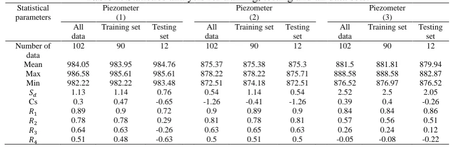
Table 2. Statistics analysis for training, testing and all data sets. Statistical parameters Piezometer (1) Piezometer (2) Piezometer (3) All data
Training set Testing set
All data
Training set Testing set
All data
Training set Testing set Number of
data
102 90 12 102 90 12 102 90 12
Mean 984.05 983.95 984.76 875.37 875.38 875.3 881.5 881.81 879.94 Max 986.58 985.61 985.61 878.22 878.22 875.71 888.58 888.58 882.87 Min 982.22 982.22 983.48 872.51 874.18 872.51 876.52 876.97 876.52
𝑆𝑑 1.13 1.14 0.76 0.54 1.14 0.54 2.52 2.5 2.05
Cs 0.3 0.47 -0.65 -1.26 -0.41 -1.26 0.39 0.4 -0.26
𝑅1 0.89 0.9 0.72 0.9 0.89 0.9 0.84 0.84 0.86
𝑅2 0.78 0.78 0.29 0.81 0.78 0.81 0.57 0.56 0.51
𝑅3 0.64 0.63 -0.26 0.63 0.65 0.63 0.26 0.24 0.12
𝑅4 0.51 0.48 -0.63 0.5 0.51 0.5 -0.05 -0.08 -0.22
Table 3. Statistics analysis for training, testing and all data sets.
Statistical parameters Piezometer (4) Piezometer (5) Piezometer (6) All data
Training set Testing set
All data
Training set Testing set
All data
Training set Testing set Number of
data
102 90 12 102 90 12 102 90 12
Mean 995.24 995.44 993.79 944.62 944.36 946.54 993.51 994 989.86 880
885 890
1 12 23 34 45 56 67 78 89
10 0 GW L ( m ) time (month) Piezometer number 7
Observed ground… 976 978 980 982 984 986 988 990 992 994 996 998
1 12 23 34 45 56 67 78 89 100
GW L ( m ) time (month) Piezometer number 8
Observed groundwater…
903 908 913
1 12 23 34 45 56 67 78 89 100
GW L ( m ) time (month) Piezometer number 9
Observed groundwater…
859 860 861 862
1 12 23 34 45 56 67 78 89 100
GW L ( m ) time (month) Piezometer number 10
AUTUMN 2016, Vol II, No II, JOURNAL OF HYDRAULIC STRUCTURES Shahid Chamran University of Ahvaz
Max 998.36 998.36 994.51 949.53 949.53 947.55 1000.92 1000.92 991.61 Min 992.83 992.83 993.04 942.51 942.51 945.22 987.51 987.51 988.64
𝑆𝑑 1.39 1.36 0.44 1.85 1.8 0.72 3.6 3.54 0.95
Cs 0.27 0.11 -0.22 1.14 1.6 -0.27 0.3 0.12 -0.3
𝑅1 0.96 0.96 0.96 0.93 0.92 0.91 0.97 0.98 0.92
𝑅2 0.9 0.89 0.83 0.85 0.83 0.74 0.94 0.94 0.74
𝑅3 0.82 0.8 -0.61 0.76 0.72 0.52 0.91 0.9 0.57
𝑅4 0.75 0.72 -0.27 0.67 0.62 0.28 0.87 0.86 -0.42
Table 4. Statistics analysis for training, testing and all data sets.
Statistical parameters
Piezomet er (7)
Piezomet er (8)
Piezomet er (9) All data Training
set
Testing set
All data Training set
Testing set All data Training set
Testing set Number of
data
102 90 12 102 90 12 102 90 12
Mean 885.04 884.7 887.65 985.1 984.75 987.71 993.51 994 989.86 Max 893.25 893.25 889.31 1039.31 997.06 1039.31 1000.92 1000.92 991.61 Min 881.27 881.27 884.25 978.39 978.39 982.46 987.51 987.51 988.64
𝑆𝑑 3.07 3.04 1.83 7.45 5.42 16.26 3.6 3.54 0.95
Cs 1.27 1.65 -0.89 4.02 0.76 3 0.3 0.12 -0.3
𝑅1 0.92 0.93 0.75 0.4 0.95 0.98 0.97 0.98 0.92
𝑅2 0.8 0.81 0.33 0.36 0.9 0.96 0.94 0.94 0.74
𝑅3 0.69 0.67 -0.17 0.51 0.84 0.93 0.91 0.9 0.57
𝑅4 0.57 0.54 -0.64 0.49 0.79 0.91 0.87 0.86 -0.42
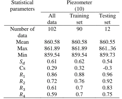
Table 5. Statistics analysis for training, testing and all data sets.
Statistical parameters
Piezometer (10) All
data
Training set
Testing set Number of
data
102 90 12
Mean 860.58 860.58 860.55 Max 861.89 861.89 861..36 Min 859.54 859.54 859.73
𝑆𝑑 0.61 0.62 0.54
Cs 0.29 0.32 -0.3
𝑅1 0.86 0.88 0.96
𝑅2 0.72 0.76 0.92
𝑅3 0.61 0.7 0.83
𝑅4 0.59 0.7 0.75
According to Table 2 to 5, the results show that piezometer (8) has a higher standard deviation compared with other piezometers and the difference between testing and training data is more than those of other piezometers.
Almost for all piezometers except piezometer (8), skewness coefficients were low for both training and testing sets. This is appropriate for modelling, because a high skewness coefficient has a considerable negative effect on the ANN performance (Altun et al., 2007).
Piezometer (8) had the most difference between all data, training and testing data.
There are more differences in lag 3 months and 4 months autocorrelation coefficient for piezometers (1), (4), (6), (7) and (9) between all data, training and testing data.
Overall, Table 2 to 5 shows a relative similarity between testing and training data and it is suitable for ANN performance. The results of our study showed that, these slight differences did not have a serious impact.
AUTUMN 2016, Vol II, No II, JOURNAL OF HYDRAULIC STRUCTURES Shahid Chamran University of Ahvaz
mapping of the variables were used. For the x variable, the scaled value x_n was computed as follows:
𝑥𝑛=(𝑥(𝑥−𝑥𝑚𝑖𝑛)
𝑚𝑎𝑥−𝑥𝑚𝑖𝑛) (1)
3. Methods
3.1. Artificial neural network analysis
The first fundamental concepts related to neural computing were developed by McCulloch and Pitts (1943). Artificial neural networks were inspired by biological findings related to the behaviour of the brain as a network of units called neurons (Rumelhart et al., 1986). A common three-layered feed-forward neural network is comprised of multiple elements, called nodes, and connection pathways that link them (Haykin, 1999). These networks contain an input layer, a hidden layer and an output layer. The input layer consists of nodes representing different input variables; the hidden layer consists of many hidden nodes; and the output layer consists of output variables. The net input to unit i is:
𝑦𝑖 = ∑𝑝𝑗=1𝑤𝑖𝑗𝑥𝑖+ 𝜃𝑖 (2)
Where 𝑤𝑗𝑖= (𝑤1, 𝑤2, … 𝑤𝑝𝑖) is the weight vector of unit 𝑖 and 𝑝 is the number of neurons in
the above layer of unit 𝑖, 𝑥𝑖 is the output from unit 𝑗 and 𝜃𝑖 is the bias of unit 𝑖. This weighted sum 𝑦𝑖, which is called the incoming signal of unit 𝑖, is then passed through a transfer function. A recommended literature for the ANN approach could be Masters (1993).
3.2. Wavelet analysis
Wavelet is a small wave energy of which is restricted to a short period of time and it is an efficient method for signals that are non-stationary, and have short-lived transient components, features at different scales, or singularities (Hsu & Li., 2010). Wavelet transform is a modern tool and a signal processing technique. It has shown a higher performance compared to the Fourier transform. The Wavelet transform performs the decomposition of a signal into a group of functions (Cohen & Kovacevic, 1996):
𝜓𝑗,𝑘(𝑥) = 2𝑗⁄2𝜓𝑗,𝑘(2𝑗𝑥 − 𝑘) (3)
Where 𝜓𝑗,𝑘(𝑥) is produced from a mother wavelet 𝜓(𝑥) which is dilated by 𝑗 and translated by 𝑘. The mother wavelet has to satisfy the condition.
∫ ψ(x)dx = 0 (4)
The discrete wavelet function of a signal f(x) can be calculated asfollows:
𝑐𝑗,𝑘 = ∫ 𝑓(𝑥)𝜓−∞∞ 𝑗,𝑘∗ (𝑥)𝑑𝑥 (5)
f(x) = ∑ cj,k j,kψj,k(x) (6)
Where, 𝑐𝑗,𝑘is the approximate coefficient of a signal. The mother wavelet is formulated from the scaling function 𝜑(𝑥) as:
φ(𝑥) = √2 ∑ ℎ0(𝑛)𝜑(2𝑥 − 𝑛) (7)
AUTUMN 2016, Vol II, No II, JOURNAL OF HYDRAULIC STRUCTURES Shahid Chamran University of Ahvaz
Where ℎ1(𝑛) = (−1)𝑛ℎ0(1 − 𝑛) . Different sets of coefficients ℎ0(𝑛) canbe found corresponding to wavelet bases with various characteristics.In the DWT, coefficients ℎ0(𝑛)play a critical role (Gupta & Gupta., 2007).
3.3. Geostatistics analysis
Geostatistics was originally developed for estimation of ore reserves in mining (Einax & Soldt., 1999). The main tool in geostatistics is the variogram, which expresses the spatial dependence between neighbouring observations. Prior to the geostatistical estimation, we require a model that enables us to compute a variogram value for any possible sampling interval. The most commonly used models are spherical, exponential, Gaussian, and pure nugget effect (Isaaks & Srivastava, 1989). The variogram quantifies the relationship between the variance and the distance between sampling pairs by the following equation (Isaaks & Srivastava, 1989, Kitanidis, 1997):
γ(h) = 1
2N(h)∑ (Z(xi+ h) − Z(xi)) 2 N(h)
i=1 (9)
Where 𝑁(ℎ) is the number of data pairs within a given class of distances and directions. And 𝑍(𝑥𝑖) and 𝑍(𝑥𝑖 + ℎ) are observations of the variable Z at spatial locations 𝑥𝑖 and 𝑥𝑖+ ℎ.
One of the geostatistics methods is the kriging technique. Only a brief description of the Kriging method is employed in this research.
3.3.1. Kriging
Kriging technique is an exact interpolation estimator 𝑍(𝑥0)used to find the best linear
unbiased estimator of a second estimator of a second order stationary. The general form of kriging equation is:
Z(x0) = ∑ni=1λiZ(xi) (10)
Where Z(𝑥0) is Kriging estimate at location𝑥0; Z(𝑥𝑖) is sampledvalue at 𝑥𝑖;𝜆𝑖 is
weighting factor for Z(𝑥𝑖); and 𝑖 = 1, . . . , 𝑛 inwhich n denotes to the numbers of samples.
4. Model application
The method proposed in this study consists of three distinct stages to achieve the best result.
For temporal GWL estimating at the first stage,
an ANN was trained and tested for each piezometer for time series modelling of the water level. The model predicted GWL of the piezometers for the next month.In the next stage, the WANN model was used. In this method, the decomposed GWL time series are entered into the ANN method for prediction of GWL one month ahead. At the end of these two-stages, the best result of these two methods were selected. And in the last stage, the spatial (GWL) was forecasted in the study area with the kriging technique.
4.1 model evaluation
Some performance evaluation criteria such as correlation coefficient are unsuitable for model evaluation (Legates & McCabe; 1999). One of the suitable criteria proposed by such researches is that a perfect evaluation of a model performance should include at least one ‘goodness-of-fit’ or relative error measure (e.g. coefficient of determination (R2)); this
AUTUMN 2016, Vol II, No II, JOURNAL OF HYDRAULIC STRUCTURES Shahid Chamran University of Ahvaz
were used to assess the effectiveness of each model. The best fit between the observed and calculated values would have R2=1, RMSE=0 and MAE=0.
R2 = 1 −∑ni=1(GWLi(measured)−GWLi(predicted))2
∑ni=1(GWLi(measured)−GWLi(mean))2
(11)
MAE =∑ni=1|GWLi(measued)−GWLi(predicted)|
n (12)
RMSE = √∑ni=1(GWLi(measured)−GWLi(predicted))2
n (13)
Where n is the number of the data points.
4.2. Application of ANN
In this study, a three-layered feed forward neural network (FFNN) with a back propagation (BP) algorithm (Masters., 1993; Haykin, 1999) was used. This algorithm is a gradient descent procedure and consists of one input layer, one hidden layer, and one output layer. The BP algorithm was employed to minimize a least-square objective function (error function). The Levenberg–Marquardt (LM) algorithm (Haykin., 1999) was used to train ANN models. The LM method is a modification of the classic Newton algorithm for finding an optimum solution to a minimization problem (Nouraniet al., 2011). The Sigmoid and Tansig (Schmitz et al., 2006) functions were used as activation functions in the hidden and output layer nodes to make the ANN model more effective. The Sigmoid function is differentiable, continuous, and monotonically increasing in its domain and it is the most frequently employed function. The numbers of the hidden layer nodes and training epochs (the training iteration number) are determined by trial and error in the test scenarios. Firstly, the training phase is completed; then, the testing phase begins using the optimum values found for the number of neurons in each input layer and hidden layer.
The artificial neural network model used in this study was the Nonlinear Auto Regressive (NAR) model
.
NAR neural networks can be trained to predict a time series from the past values of that series.4.3. Application of WANN
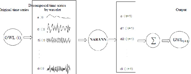
In the WANN model, the decomposed GWL time series was linked to the ANN method for the prediction of GWL one month ahead. The proposed WANN model for the prediction of GWL is shown in Fig. 3.
AUTUMN 2016, Vol II, No II, JOURNAL OF HYDRAULIC STRUCTURES Shahid Chamran University of Ahvaz
Correlation analysis (that is considered in ANN model inputs) provides information on the global functioning of GWL time series, but cannot take the temporal variability of the time series into account, which often leads to a nonlinear and nonstationary functioning of the presses. Therefore, the wavelet approach was presented to focus on the non-stationary properties of time series. The unknown periodical characteristics of GWL time series could be detected using theWANN model (Rajaee., 2011).
Firstly, GWL time series were decomposed to some multi-frequently time series by a discrete wavelet transform; then at the next step, decomposed time series at different scales were entered into the ANN for predicting GWL one month ahead. In wavelet analysis, selecting an appropriate wavelet function called “mother wavelet” is an important step. In this study, the sensitivity of the decomposed level is investigated. The GWL time series was decomposed to 1,2,3,4 levels; for example, the level 4 decomposition of the GWL signal yields five sub-signals (approximation at level 4 and detail at levels 1, 2 and 3) by a different kind of transform (i.e. Haar wavelet (a simple wavelet), Daubechies-2 (db2) wavelet (a most popular wavelet) (Mallat., 1989)
(
.4.4 Application of kriging
In this stage, in order to estimate GWL one month ahead at unsample spatial locations such as locations without piezometers or locations with no possibility of direct observation of GWL, the results of the two previous stages were used. At the first step of this stage, the data normalized by Eq. (1) were used in the kriging methods, and the variogram of these data were calculated. The varigram provided a way to study the influence of the factors that may affect the influence of other factors that determine whether the spatial correlation varies only with distance (the isotropic case) or with direction and distance (the anisotropic case). Variogram maps provide a visual picture of semivariance in every compass direction. If there is anisotropy, this allows one to easily find the appropriate principal axis for defining the anisotropic variogram model (Nourani et al., 2011). Thereafter, a suitable experimental varigram (i.e. spherical, Gaussian, exponential etc.) was determined by using weighted least-squares (Myers, 1982).
5. Result and discussion
AUTUMN 2016, Vol II, No II, JOURNAL OF HYDRAULIC STRUCTURES Shahid Chamran University of Ahvaz
Table 6. 𝑅2, MAE and RMSE values in GWL prediction by ANN models in a testing period.
piezometer ANN structures 𝑅2 RMSE MAE P1 1-3-1 0.401 0.388 0.251 P2 1-5-1 0.676 0.21 0.292 P3 1-3-1 0.63 1.244 1.015 P4 1-4-1 0.696 0.232 0.203 P5 1-3-1 0.439 0.514 0.445 P6 1-3-1 0.699 0.496 0.367 P7 1-3-1 0.668 1.007 0.882 P8 1-4-1 0.744 0.277 0.224 P9 1-4-1 0.445 0.215 0.17 P10 1-3-1 0.722 0.27 0.224
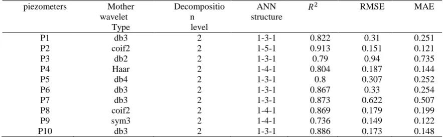
For the performance evaluation of the WANN in prediction of GWL, a dataset normalized by Eq. (1) was decomposed into sub-series using a discrete wavelet transform. One of the important steps in this stage is the determination of mother wavelet type and optimum decomposition level. The nature of the phenomenon and the type of the time series are important factors for selecting the mother wavelet. The functions of the mother wavelet have different types. In this research different kinds of the mother wavelet (e.g. Haar, Daubechies, Symlets, Coiflets, Biorthogonal, Reverse biorthogonal) were tested to achieve the best results.
After determining the mother wavelet, selecting the appropriate level of decomposition was the next step; to achieve this purpose, the following experimental formula was used to determine the level of optimum decomposition:
l = int[log(𝑛)] (14)
Where n is the length of the time series, int[] stands for the integer function and log() is the common logarithm (Wang & Ding, 2003).
The results showed that the level 2 can be considered as an appropriate decomposition level, and by increasing the decomposition level, in levels greater than 2, the model performance decreased because high decomposition levels lead to a large number of parameters with complex nonlinear relationships in the ANN approach (Rajaee., 2011).
For each piezometer, the obtained sub-signals were separately applied to the network. Finally, the sum of the predicted values showed the end result for each piezometer. In the next stage, the obtained results from wavelet transform were linked to the ANN method for prediction of GWL one month ahead.. The results of the WANN model for the existing piezometers are presented in Table 7.
Table 7. 𝑅2, RMSE and MAE in GWL prediction by the WANN model in the testing period.
piezometers Mother wavelet
Type
Decompositio n level
ANN structure
𝑅2 RMSE MAE
AUTUMN 2016, Vol II, No II, JOURNAL OF HYDRAULIC STRUCTURES Shahid Chamran University of Ahvaz
Table 7 shows quite suitable results. However, gaining accurate results requires precise information about effective factors. It can be concluded that the groundwater level depends on various factors which are not based on accurate statistics and it becomes a complex process because of the interference of different phenomena. This relationship cannot be written in the in the form of a mathematical equation, even though there is enough statistical information about these factors. The cause of this phenomena cannot be stated clearly due to the complexity and nonlinearity of the models of neural network.
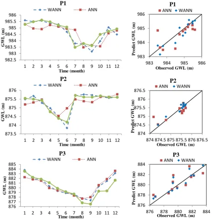
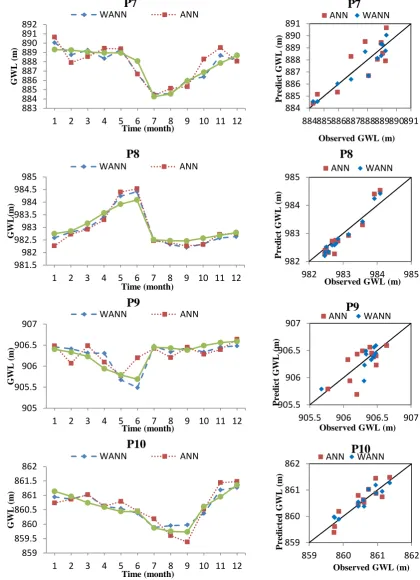
The results of the ANN and WANN models are presented in Fig. 5, which demonstrates the capability of the ANN model and, according to the scatter-plots, a comparison between WANN and ANN model showed a better performance of the WANN model.
982.5 983 983.5 984 984.5 985 985.5 986
1 2 3 4 5 6 7 8 9 10 11 12
G W L (m ) Time (month)
P1
WANN ANN 983 984 985 986983 984 985 986
Pre d ict G W L (m )
Observed GWL (m)
P1
ANN WANN 873.5 874 874.5 875 875.5 8761 2 3 4 5 6 7 8 9 10 11 12
G W L (m ) Time (month)
P2
WANN ANN 874 874.5 875 875.5 876 876.5874 874.5 875 875.5 876 876.5
Pre d ict G W L (m )
Observed GWL (m)
P2
ANN WANN 876 877 878 879 880 881 882 883 884 8851 2 3 4 5 6 7 8 9 10 11 12
G W L (m ) Time (month)
P3
WANN ANN 876 878 880 882 884876 878 880 882 884
Pre d ict G W L (m )
Observed GWL (m)
P3
AUTUMN 2016, Vol II, No II, JOURNAL OF HYDRAULIC STRUCTURES Shahid Chamran University of Ahvaz
992.5 993 993.5 994 994.5 995
1 2 3 4 5 6 7 8 9 10 11 12
G W L (m ) Time (month)
P4
Series1 Series2 992.5 993 993.5 994 994.5 995992.5 993 993.5 994 994.5 995
Pre d ict G W L (m )
Observed GWL (m)
P4
ANN WANN 944.5 945 945.5 946 946.5 947 947.5 9481 2 3 4 5 6 7 8 9 10 11 12
G W L (m ) Time (month)
P5
WANN ANN 944.5 945.5 946.5 947.5 948.5944.5 945.5 946.5 947.5 948.5
Pre d ict G W L (m )
Observed GWL (m)
P5
ANN WANN 988 988.5 989 989.5 990 990.5 991 991.5 9921 2 3 4 5 6 7 8 9 10 11 12
G W L (m ) Time (month)
P6
WANN ANN 988 989 990 991 992988 989 990 991 992
Pre d ict G W L (m )
Observed GWL (m)
P6
AUTUMN 2016, Vol II, No II, JOURNAL OF HYDRAULIC STRUCTURES Shahid Chamran University of Ahvaz
Fig 4. Comparisons between the measured and predicted GWL based on the testing data.
883 884 885 886 887 888 889 890 891 892
1 2 3 4 5 6 7 8 9 10 11 12
G W L (m ) Time (month)
P7
WANN ANN 884 885 886 887 888 889 890 891 884885886887888889890891 Pre d ict G W L (m )Observed GWL (m)
P7
ANN WANN 981.5 982 982.5 983 983.5 984 984.5 9851 2 3 4 5 6 7 8 9 10 11 12
GW L(m ) Time (month)
P8
WANN ANN 982 983 984 985982 983 984 985
Pre d ict G W L (m )
Observed GWL (m)
P8
ANN WANN 905 905.5 906 906.5 9071 2 3 4 5 6 7 8 9 10 11 12
G W L (m ) Time (month)
P9
WANN ANN 905.5 906 906.5 907905.5 906 906.5 907
Pre d ict G W L (m )
Observed GWL (m)
P9
ANN WANN 859 859.5 860 860.5 861 861.5 8621 2 3 4 5 6 7 8 9 10 11 12
G W L (m ) Time (month)
P10
WANN ANN 859 860 861 862859 860 861 862
Pre d icte d G W L (m )
Observed GWL (m)
P10
AUTUMN 2016, Vol II, No II, JOURNAL OF HYDRAULIC STRUCTURES Shahid Chamran University of Ahvaz
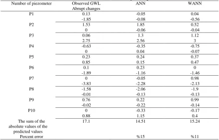
Anticipated maximum and minimum points of GWL are important in the design of hydraulic structures, and it can be a good feature of the hydrological model. Table 8 compares the performance of these two models. According to this table, in this part, the WANN model has better results, too.
Table 8. Performance of models to forecast the peak of groundwater level.
Number of piezometer Observed GWL Abrupt changes
ANN WANN
P1 0.13 -0.05 0.04
-1.85 -0.08 -0.56
P2 1.53 1.85 0.52
0 -0.06 -0.04
P3 0.06 1.3 1.12
2.75 2.56 3
P4 -0.63 -0.35 -0.75
0 0.04 -0.07
P5 0.23 0.24 0.37
0.85 0.15 0.47
P6 0.1 0.23 0
-1.89 -1.16 -1.46
P7 0 -0.05 0.98
-3.83 -2.28 -2.13
P8 -1.58 -2.06 -1.9
-0.01 -0.13 -0.13
P9 0.76 0.22 0.99
-0.02 -0.22 -0.14
P10 0 -0.33 -0.17
0.88 1.15 0.4
The sum of the absolute values of the
predicted values
17.1 14.51 15.24
Percent error %15 %11
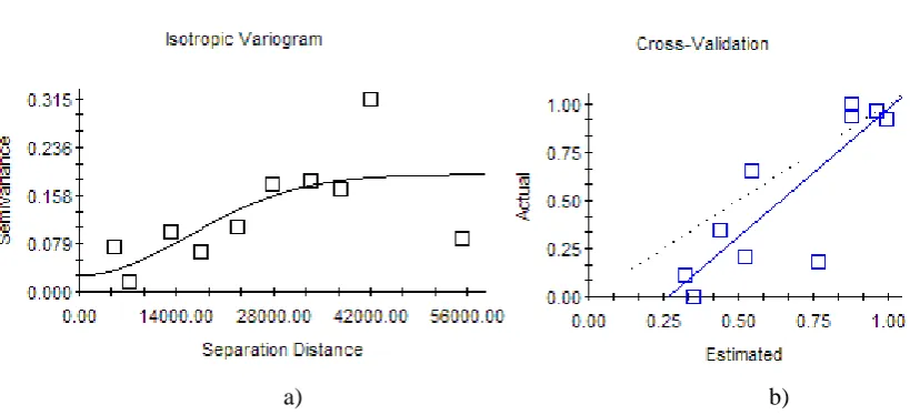
According to the best results obtained in the previous steps, the best variogram of the data was plotted using the values of the GWLs at different piezometers. An appropriate variogram model was plotted by fitting such variogram models. The geostatistical model, which leads to the least RMSE was selected by comparing the observed GWL values with the values estimated by variogram models (Nourani et al, 2011).
The results of the best-fitted model are presented in Table 9; this model is selected based on the least values of RMSE and RSS among other models.
Table 9.Rresults of different variogram models.
Model RMSE
Spherical 0.260 *Gaussian 0.253 Exponential 0.268 Linear 1.005
AUTUMN 2016, Vol II, No II, JOURNAL OF HYDRAULIC STRUCTURES Shahid Chamran University of Ahvaz
a) b)
Fig 5. (a) Selected variogram model. (b) Cross validation results.
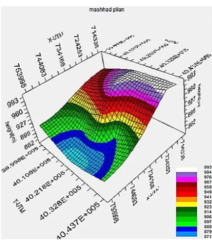
Table 10 shows real groundwater level and the percent error compared to the predicted value. Ultimately, the best results of the previous stages for one month ahead are shown in Fig.7. Fig.7 shows the groundwater level in the study area according to the legend of figure.
Table 10.Compare groundwater level forecasting with real groundwater level
Number of piezometer Groundwater level forecasting in one month
ahead (m)
Percent error
P1 984.9 0.13
P2 875.63 0.34
P3 884.98 0.08
P4 994.17 0.04
P5 947.24 0.43
P6 987.85 0.01
P7 888.77 0.91
P8 982.58 0.28
P9 906.53 0.35
P10 861.35 0.14
Estimation of GWL is dependent on many factors. There is not accurate statistics for these factors. Dependence on many various factors causes a complicate relationship. According to the results of the temporal forecasting, good results of hybrid model wavelet-artificial neural network and also due to the obtained delays, this model has established a relationship with achieved delays.
AUTUMN 2016, Vol II, No II, JOURNAL OF HYDRAULIC STRUCTURES Shahid Chamran University of Ahvaz
Fig 7. groundwater level forecasting in study area
6. Summary and conclusion
In the current study, an attempt was made to investigate the capability of the proposed hybrid empirical models for spatiotemporal GWL forecasting. This model was applied for Mashhad City and its environs in the Northeast Iran at Khorasan Razavi Province. Firstly, for temporal forecasting stage by comparison of the prediction accuracies of ANN and WANN models indicated that the proposed WANN model with coefficient of determination and root mean square error and mean absolute error, 0.836 and 0.335 and 0.273 respectively, showed better results. GWL signals were decomposed into sub-signals with different scales, and this decomposed GWL time series was used as input data to the ANN models for prediction of GWL one month ahead. The results showed that the right choice of the mother wavelet and optimum decomposed level lead to a more precise prediction, and increasing the decomposition level, lead to low efficiency.
Then, in the spatial estimation stage, the kriging method was applied to the outputs from the WANN models to estimate GWL in the environs of Mashhad City one month ahead, especially in unsampled locations. A Gaussian model with 0.253 in RMSE had the best result among other variograms.
In order to extend the presented model, adding some forecasting sub-models for modelling the input hydrological parameters of the model such as temperature or precipitation intensity or evapotranspiration or using other interpolation methods in geostatistics like Cokriging or Spline or Inverse Distance Weighting (IDW) is recommended for future researches.
References
1. Rajaee, T., 2011. Wavelet and ANN combination model for prediction of daily suspended sediment load in rivers. Science of the Total Environment, 409: 2917–2928.
AUTUMN 2016, Vol II, No II, JOURNAL OF HYDRAULIC STRUCTURES Shahid Chamran University of Ahvaz
3. Ravansalar, M., Rajaee, T., 2015. Evaluation of Wavelet Performance via an ANN-Based Electrical Conductivity Prediction model. Environmental Monitoring and Assessment 187:366. DOI 10.1007/s10661-015-4590-7.
4. Yang, Z.P., Lu, W.X., Long, Y.Q., Li, P., 2009. Application and comparison of two prediction models for groundwater levels: A case study in Western Jilin Province, China. Journal of Arid Environments, 73: 487–492.
5. Shiri, J., Kisi, O., 2011. Comparison of genetic programming with neuro-fuzzy systems for predicting short-term water table depth fluctuations. Computers and Geosciences, 37: 1692-1701.
6. Yoon, H., Jun, S., Hyun, Y., Bae, G., Lee, K., 2011. A comparative study of artificial neural networks and support vector machines for predicting groundwater levels in a coastal aquifer. Journal of Hydrology, 396: 128–138.
7. Mohammadi, K., 2008. Groundwater table estimation using MODFLOW and artificial neural networks. Water Science and Technology Library 68, no. 2: 127-138.
8. Nourani, V., Goli Ejlali, R, and Alami, M.T., 2011. Spatiotemporal Groundwater Level Forecasting in Coastal Aquifers by Hybrid Artificial Neural Network-Geostatistics Model: A Case Study. Environmental Engineering Science, 28(3): 217-228.
9. Nakhaei, M., Saberi Nasr, A., 2012. A combined Wavelet- Artificial Neural Network model and its application to the prediction of groundwater level fluctuations. Geopersia, 2 (2): 77-91.
10. Zhou, H.C., Peng, Y., Liang, G.H., 2008. The research of monthly discharge predictor-corrector model based on wavelet decomposition. Water ResourcesManagement, 22: 217– 227.
11. Kisi, O., 2010. Wavelet regression model for short-term streamflow forecasting. Journal of Hydrology 389: 344–353.
12. Gemitzi, A., Stefanopoulos, K., 2011. Evaluation of the effects of climate and man intervention on ground waters and their dependent ecosystems using time series analysis. Journal of Hydrology 403: 130–140.
13. Wang, W., Jin, J., Li, Y, 2009. Prediction of inflow at three gorges dam in Yangtze river with wavelet network model. Water Resources Management, 23: 2791–2083.
14. Sahoo GB, Ray C, Mehnert E, Keefer DA., 2006. Application of artificial neural networks toassess pesticide contamination in shallow groundwater. Sci Total Environ, 367:234–51. 15. Rajaee T, Mirbagheri SA, Zounemat-Kermani M, Nourani V., 2009. Daily suspended
sedimentconcentration simulation using ANN and neuro-fuzzy models. Sci Total Environ, 407:4916–27.
16. Tsai CH, Chang LC, Chiang HC., 2009. Forecasting of ozone episode days by cost-sensitiveneural network methods. Sci Total Environ. 407:2124–35.
17. Aziz, A.R.A., Wang, K.F.V., 1992. Neural networks approach the determination of aquifer parameter. Groundwater, 30(2): 164-166.
18. Lallahem, S., Mania, J., Hani, A., Najjar, Y., 2005.On the use of neural networks to evaluate groundwater levels in fractured media. Journal of Hydrology, 307: 92–111.
19. Daliakopoulos, I.N., Coulibaly, P., Tsanis, I.K., 2005. Groundwater level forecasting using artificial neural networks. Journal of Hydrology, 309: 229–240.
AUTUMN 2016, Vol II, No II, JOURNAL OF HYDRAULIC STRUCTURES Shahid Chamran University of Ahvaz
21. Sahoo, S., Jha, MK., 2013. Groundwater-level prediction using multiple linear regression and artificial neural network techniques: a comparative assessment. Hydrogeology Journal. 21(8): 1865-1887.
22. Maiti, S., Tiwari, R. K., 2014. A comparative study of artificial neural networks, Bayesian neural networks and adaptive neuro-fuzzy inference system in groundwater level prediction. Environmental Earth Sciences. 71(7): 3147-3160.
23. Pasquini A, Depetris P., 2007. Discharge trends and flow dynamics of South American riversdraining the southern Atlantic seaboard: an overview. Journal of Hydrology, 333:385– 99.
24. Rajaee T., 2010. Wavelet and neuro-fuzzy conjunction approach for suspended sediment prediction. Clean-Soli, Air, Water, 38(3):275–86.
25. Shoaib M, Shamseldin A.Y, Melville B.W., 2014. Comparative study of different wavelet based neural network models for rainfall–runoff modeling. Journal of Hydrology, 515: 47– 58.
26. Nourani V, HosseiniBaghanam A, Adamowski J, Kisi O., 2014. Applications of hybrid wavelet–Artificial Intelligence models in hydrology: A review. Journal of Hydrology, 514: 358–377.
27. Adamowski, J., Chan, H.F., 2011. A wavelet neural network conjunction model for groundwater level forecasting. Journal of Hydrology, 407: 28–40.
28. Nourani, V., Alami, M., Aminfar, M., 2009.A combined neural-wavelet model for prediction of Ligvanchai watershed precipitation. Engineering applications of Artificial Intelligence, 22: 466–472.
29. Rouhani, Sh., & Meyers, D. E., 1990. Problems in space-time kriging of geohydrological data. Mathematical Geology,22:611–623.
30. Reghunath, R., Sreedhara Murthy, T. R., & Raghavan, B. R., 2005. Time series analysis to monitor and assess water resources: A moving average approach. Environmental Monitoring and Assessment, 109:65–72.
31. Kumar, S., Sondhi, S. K., &Phogat, V., 2005. Network designfor groundwater level monitoring in upper Bari Doab canaltract, Punjab, India. Irrigation and Drainage, 54:431– 442.
32. Abedian H, Mohammadi K, Rafiee R., 2013. Optimizing monitoring network of water table by geostatistical methods. Journal of Geology and Mining Research, 5(9): 223-231.
33. Kholghi M, Hosseini S.M., 2009. Comparison of Groundwater Level Estimation Using Neuro -fuzzy and Ordinary Kriging. Environmental Modelling& Assessment, 14(6): 729-737.
34. Altun H, Bilgil A, FidanBC.,2007. Treatment of multi-dimensional data to enhance neural network estimators in regression problems. Expert SystAppl, 32(2):599–605.
35. McCulloch WS, Pitts WH., 1943. A logical calculus of the ideas immanent in neural nets. BullMathBiophys, 5:115–33.
36. Rumelhart, D.E., and McClelland, J.L., 1986. Parallel DistributedProcessing: Explorations in the Microstructure of Cognition, I andIi. Cambridge: MIT Press.
37. Haykin S., 1999. Neural network — a comprehensive foundation. Englewood Cliffs, NJ:Prentice-Hall.
AUTUMN 2016, Vol II, No II, JOURNAL OF HYDRAULIC STRUCTURES Shahid Chamran University of Ahvaz
39. Hsu, K.C., Li, S.T., 2010. Clustering spatial–temporal precipitation data using wavelet transform and self-organizing map neural network. Advances in Water Resources 33: 190-200.
40. Cohen A, Kovacevic J., 1996. Wavelets: the mathematical background. Proc IEEE, 84(4):514–22.
41. Gupta KK, Gupta R., 2007.Despeckle and geographical feature extraction in SAR images bywavelet transform. ISPRS J Photogramm, 62(6):473–84.
42. Einax JW, Soldt U., 1999. Geostatistical and multivariate statistical methods for the assessment of polluted soils-merits and limitations.Chemom. Intell. Lab. Syst, 46: 79-91. 43. Isaaks, E.H., and Srivastava, R.M., 1989. Applied Geostatistics. New York: Oxford
University Press.
44. Kitanidis, P. K., 1997. Introduction to geostatistics: Application to hydrogeology. Cambridge, UK: Cambridge University Press.
45. Legates DR, McCabe JrGJ., 1999. Evaluating the use of goodness-of-fit measures in hydrologicandhydroclimatic model validation. Water Resour Res. 35(1):233–41.
46. Nash, J.E., and Sutcliffe, J.V., 1970. River flow forecastingthrough conceptual models: part I. A conceptual models discussionof principles. J. Hydrol, 10, 282.
47. Schmitz J. E, Zemp R. J, Mendes M.J., 2006. Artificial neural networks for the solution of the phasestability problem. Fluid Phase Equilib, 245:83–7.
48. Mallat S.G., 1989. A theory for multi resolution signal decomposition: the wavelet representation. IEEE Trans Pattern Anal Mach Intell, 11(7):674–93.
49. Abrahart RJ, See L., 2000. Comparing neural network (NN) and Auto Regressive Moving Average (ARMA) techniques for the provision of continuous river flow forecasts in two contrasting catchments. Hydrol Process, 14:2157–72.