Observing desert dust devils with a pressure logger

Geosci. Instrum. Method. Data Syst., 1, 209–220, 2012 www.geosci-instrum-method-data-syst.net/1/209/2012/ doi:10.5194/gi-1-209-2012

© Author(s) 2012. CC Attribution 3.0 License.

Geoscientific

Methods and

Data Systems

Geoscientific

Methods and

Data Systems

Observing desert dust devils with a pressure logger

R. D. Lorenz

Johns Hopkins University Applied Physics Laboratory, Laurel, MD 20723, USA

Correspondence to: R. D. Lorenz ([email protected])

Received: 2 July 2012 – Published in Geosci. Instrum. Method. Data Syst. Discuss.: 17 July 2012 Revised: 12 November 2012 – Accepted: 13 November 2012 – Published: 4 December 2012

Abstract. A commercial pressure logger has been adapted for long-term field use. Its flash memory affords the large data volume to allow months of pressure measurements to be acquired at the rapid cadence (>1 Hz) required to detect dust devils, small dust-laden convective vortices observed in arid regions. The power consumption of the unit is studied and battery and solar/battery options evaluated for long-term ob-servations. A two-month long field test is described, and sev-eral example dust devil encounters are examined. In addition, a periodic (∼20 min) convective signature is observed, and some lessons in operations and correction of data for tem-perature drift are reported. The unit shows promise for ob-taining good statistics on dust devil pressure drops, to permit comparison with Mars lander measurements, and for array measurements.

1 Introduction

Dust devils (e.g., Balme and Greeley, 2006) are vertical con-vective vortices encountered in arid regions, in particular dur-ing periods of strong solar heatdur-ing (early afternoon in sum-mer). The vortical structure is rendered visible by lofted dust, which may (via sunlight absorption) itself contribute to the strength of the convection intensity.

Pressure drops in dust devils have been noted in the past on Earth (e.g., Wyett, 1954; Lambeth, 1966; Sinclair, 1973), but are actually more systematically documented in studies of dust devils on Mars (e.g., by Mars Pathfinder: Murphy and Nelli, 2002, and by the Phoenix lander, Ellehoj et al., 2010), where landers have recorded meteorological parameters over long periods with a high enough cadence to detect small vor-tical structures. A number of dust-devil type vortices were detected by the Viking lander (via wind speed and direction, e.g., Ryan and Lucich, 1983 – the pressure measurements

were acquired too infrequently to be of use in this applica-tion). Interest in further measurements remains high – vari-ous proposals for network missions (including pressure sens-ing) have been made such as NASA’s MESUR, the French Netlander, and recently the Finnish METNET. The NASA rover Curiosity, which landed on Mars in August 2012, car-ries a meteorology package, as will the recently-selected NASA Insight mission to be launched in 2016. All these mis-sions may detect dust devils on Mars via pressure records and other data.

Routine terrestrial meteorological stations only record data at∼15 min cadence, too infrequently to detect dust dev-ils. As discussed in Lorenz (2012), it would be highly desir-able to obtain a dataset of∼1 Hz or better fixed-station pres-sure data at a place and time where dust devils are known to occur. Such a dataset should last several weeks (Mars perience suggests of order one encounter per day can be ex-pected, so several months of operation of a single station are needed) in order to obtain a useful number of dust devil en-counters (i.e., of order a hundred or more, to permit robust comparison with Mars). While mobile measurement plat-forms (e.g., Sinclair, 1973) can obtain a larger number of encounters in a given time, they do so at considerable ex-pense in labor, and at the cost of introducing selection bias in the dust devils encountered (largest, slowest, etc.) and with possible vehicle effects on part or all of the record.

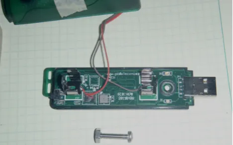
logger by Gulf Coast Data Concepts. The unit (Fig. 1) is es-sentially a small circuit board with a USB connector for data transfer: all components (including the pressure sensor, a re-set switch, and a holder for a AA battery) are mounted on this board, which is protected by a three-part semitransparent plastic housing. The housing is about 2.5 cm in diameter and 10 cm long: with the AA battery installed, the unit weighs only 55 g.

The product literature (GCDC, 2010) reports that the unit will run for 3 weeks on an alkaline AA cell. This, however, appears to be only at a low sample rate. A requirement for detecting small dust devils, distinct from more general me-teorological investigations, is that samples be acquired at a high rate of one sample per second or better. Our initial tests showed that an alkaline AA cell will last only a few days at the highest rate of 10 Hz, although at 1–2 Hz sampling about 10 days of continuous operation can be expected.

The logger stores readings acquired at rate up to 10 Hz in a comma-delimited text file (CSV), with a timestamp for each reading. These files are written as ASCII text files to a 2 GB micro-SD flash memory card. This card is also used to hold a configuration file which determines the sample rate, file size, etc. The sensor (Bosch Sensortech, 2009) in the unit is a BMP-085 Digital Pressure Sensor by Bosch Sensortec, in a 5×5×1.2 mm package which communi-cates with the B1100 microcontroller using an I2C interface and has a nominal resolution of 0.01 mb. The BMP-085 is factory-programmed with 11 16-bit constants that are used, together with an on-chip temperature measurement, by the microcontroller to correct the raw pressure reading into a cal-ibrated value.

2.2 Data storage

The ASCII file written by the loggers is less compact than a binary format, but considerably more convenient in most applications. A header contains the unit serial number, the file origination time, battery voltage and setting information, then a user-specified number of measurement lines follow, with each line containing the measurement time in decimal seconds after the file origination time, and the pressure read-ing in Pascals as an integer, and optionally (see below) an integer temperature reading in tenths of a degree Celsius.

A file with 86 400 measurements (i.e., a day of data at 1 sample per second) occupies 1.5 MB: even at the maximum

Fig. 1. Datalogger with the casing partly removed. The USB con-nector is at right, the AA battery terminals are visible at right and left (with user-supplied wires soldered there to provide an alterna-tive power supply in this application). The pressure transducer is the silver square at the lower edge of the board. The memory, micro-controller and other components are on the other side of the circuit board.

sample rate of 10 Hz, about 4 months of data could be stored in the 2 GB card supplied with the unit. Note that the filesystem on the logger only records 999 data files. While large datafiles can be inconvenient (e.g., at least some ver-sions of Microsoft Excel have difficulties plotting more than 32 768 points, and code in IDL or a similar language needs loop or index variables to be of long integer type), it may be necessary to use large files if high sample rates are in-tended for long periods of observation in order to keep the total number of files below 1000.

Several additional pieces of information are stored. First, the battery voltage is recorded in the header of the file. Sec-ondly, every 100 pressure readings (or at some other interval – it is specified by the user in the configuration file) a tem-perature reading is written. Since the temtem-perature sensor is simply on the circuit board, it has too high a thermal inertia to respond quickly to air temperature changes and thus is not of particular interest in dust devil measurements directly. In-cluding the temperature data adds five characters to each line (a three digit temperature reading plus a space and comma), which typically is 12–16 characters long with the time and pressure reading, i.e., it imposes a 20–30 % data overhead; thus, to include the temperature data at every reading would reduce the number of pressure readings that could be accom-modated in the flash memory. Thus, since the temperature data were not expected to be of immediate meteorological interest, an interval of 100 readings was chosen; we will re-turn to this decision later.

Fig. 2. Discharge curve of a Duracell alkaline AA cell (50 mA constant current) from manufacturer’s datasheet (circles), compared

with a simple analytic modelC= Co/[1 + exp{(V −V o)/dV}]with

Co = 2.2 A-h, Vo = 1.25 V and dV= 0.07 V (solid line). Where this

curve intersects the voltage threshold of the logger (dotted line), the unit stops – in this case (threshold = 1.25 V) after a discharge of about 1 A-h – even though substantial capacity remains. One miti-gation is to put two cells in series (dashed curve) – here the curve intersects the threshold after some 2.2 A-h. The rather shallow dis-charge curve of alkaline cells means that if the threshold is even slightly higher, a significant drop in useful battery capacity results.

be synchronized with modest effort and care in setting the clock for each unit. Since each clock can be set from the same PC, an initial synchronization to about 1 s should be achievable (no attempt has been made to evaluate the clock performance.)

2.3 Power consumption

It was noted in initial tests that the logger ceased operation when the battery voltage fell to about∼1.25 V. For conven-tional alkaline batteries, this in fact means there is consid-erable capacity left in the cell (see Fig. 2). Inquiries with the manufacturer indicated that a∼1.2 V cut-off was intro-duced to avoid brownout of the system during file-write op-erations to the SD card, when the current draw can increase momentarily up to 100 mA. Corruption of the file system can result if the voltage drops too low under this current draw, and thus operations are suppressed when the voltage is low enough that this might be a risk. In fact, we have noted sim-ilar problems (and in fact introduced a simsim-ilar precaution to cease operations before battery voltage fell too low) in ex-periments with digital time-lapse cameras used to study dust devils (Lorenz et al., 2010).

The device (Alex Kooney, personal communication, 2012) uses a boost regulator to generate a 3.3 V operating voltage from the battery supply. Because of this boost operation, cur-rent consumption decreases for higher battery voltage, which can be higher than 1.5 V (although no advantage is gained above 3.3 V). We have measured the current consumption for 1.5 V and 3.0 V supplies and list the results in Table 1;

Table 1. B1100-1 Current consumption for one fresh alkaline cell and two cells in series.

Samples Current Current Current

per draw draw draw

second (mA) (mA) (mA)

1.5 V 1.5 V 3.0 V

supply supply supply

LEDs on LEDs off LEDs on

1 7.0 6.7 4.0

2 7.4 7.3 4.0

5 11.0 7.7

3.3 15.4

10 17.0 16.0 9.3

indeed, for a given sample rate the current draw is reduced by a factor of just under two for the higher supply voltage. The unit’s configuration file also allows the user to disable the indicator LEDs – this change makes only a modest (∼5 %) difference in consumption. For the 1.5 V supply, the current varies roughly linearlyI= 6 + 1.1 s, where s is the sample rate in Hz andI the current in mA. Note that the currents in Ta-ble 1 are the typical values; there are brief spikes during flash write operations that are not accounted for.

Thus, our approach to enhancing the longevity of the sys-tem is threefold. First, two alkaline cells are used in series. This reduces the current consumption due to the (typically) higher supply voltage, which introduces a factor of nearly two increase in endurance. Second, because the discharge curve of two cells in series only reaches 1.25 V when the cells have been almost completely depleted (∼2.1 A-h, com-pared with∼0.8 A-h for a single cell to 1.25 V, see Fig. 2), an additional factor of∼2.5 is obtained. Finally, larger (D) cells are used, bringing a final additional factor of∼6–10 over AA cells. Thus, the total endurance is enhanced by∼30 compared with the single AA cell by the substitution of 2-D cells with a battery holder, totaling about $ 5 per unit. The logger andDcells/holders fit inside a “2.5-cup” polypropy-lene food container, sprayed with sand-textured paint for this application (see Fig. 3). Note that a hole must be drilled in this waterproof housing to permit external pressure changes to be rapidly communicated to the sensor and to prevent tem-perature changes causing the internal pressure to vary.

Fig. 3. Sand-colored waterproof food container used to house 2-D cells and the pressure logger for field measurements.

the power consumption by a factor of 3–4. Because extended cloudy periods may allow the secondary battery to become temporarily exhausted (which would reset the datalogger and stop its operation), this approach was adopted in parallel with a pair of alkaline AA cells as backup. This is particularly important since Nickel Cadmium (NiCd) rechargeable cells perform poorly at the very high temperatures encountered by dust devil survey instrumentation. The solar cell charged a set of 3 NiCd AA cells (thus a nominal 3.6 V dropped to 3 V at the logger power terminals by a 1N4148 diode in series; a similar diode in series with the alkaline cells isolated them unless the NiCd voltage fell below 2.4 V).

2.4 Design for measurement campaign

We now have the information at hand to best configure the system for field use. For a 1 week campaign, a single AA cell will suffice if 2 Hz data is adequate; for 10 Hz data 2×AA or 1×Dcell must be used. For a 1 month campaign, 2×AA or 1×Dwill allow 2 Hz data, but the 2×Doption must be exercised for 10 Hz data. For a 4-month campaign, the 2×D

cell (or solar) options are needed, and will permit 10 Hz data. Note, however, in these cases and for longer measurements, the data storage becomes the limiting factor. As indicated in Sect. 2.2 above, 4 months of operation at 10 Hz will fill the 2 GB memory. Note also that 4 months (∼1E7s) corresponds to 1E8 lines of data, so the 1000-file limit of the file system would require that each file exceed 100 000 lines in length.

3 Field trial

Three units were deployed on 16 April 2012 on a playa (dry lake bed) in southern Nevada (Fig. 4), a location known (e.g., Pathare et al., 2010) to see dust devil activity. Each was set at the foot of a small sagebrush (Fig. 5), which provided some

Fig. 4. The playa (about 6 km long) seen from a commercial air-liner approaching Las Vegas. The approximate measurement site is arrowed. Highway I-95 runs roughly north–south. The blueish rect-angular feature at left is a solar power facility.

Fig. 5. Sagebrush patch on the playa with solar-powered datalogger installed.

shelter from wind and some concealment, and the location recorded with GPS. Two units (“P10” and “P16”) were pow-ered by alkaline D-cells, and the other (“P15”) by three AA NiCd cells recharged with a solar cell and with a 2 AA-alkaline cell backup. The units were left unattended until recovered on 21 May 2012; the initial measurement period was therefore 35 days. At this point data were downloaded, and another battery unit (“P12”) was deployed and opera-tions continued for another three weeks until the surviving units were recovered on 11 June 2012.

All three units operated successfully for the first mea-surement duration and some 2 Gbit of data were obtained. Contemporaneous hourly meteorological data were obtained from the Remote Automatic Weather Station (RAWS) at Red Rock Canyon, about 10 km to the northeast, which is not dis-cussed further in the present paper.

Fig. 6. Battery voltage at the start of each datafile recorded by the three sensors in April 2012. Note the steep initial decline (compare with Fig. 2) for the top two alkaline-only units. Note the slower decline for P16, with the lower sample rate. The lowest unit shows a generally uniform diurnal cycle, although peak voltage dropped on days 9 and 10 due to clouds.

Three units and another ∼2 GB of data were obtained when the site was visited in early June 2012. Unfortunately the solar-powered unit was not present, presumably removed by unknown persons (the playa is frequented for various recreational activities, including drag racing, flying radio controlled airplanes, etc.). Perhaps the necessity of main-taining a clear sky view to obtain solar power made this installation particularly visible to passersby. It may be that the penalty of finite battery lifetime is worth the reduced probability of theft or damage by better concealment (or even burial) that is impossible for solar-powered installa-tions. Similarly, adding a prominent notice “Scientific Equip-ment, Please Leave Undisturbed” may decrease the proba-bility of interference or removal if the unit is found, but in-creases the probability of it being noticed in the first place.

4 Field data and noise performance

The absolute calibration of the unit is not important for the present application although the manufacturer’s data sheets (Bosch Sensortech, 2009; GCDC, 2010) quotes 1 hPa (i.e., ∼1 mb). The noise level depends on the measurement mode and is quoted as 3–6 Pa or 0.03 mb. The reading is output as an integer in Pa (i.e., a resolution of 1 Pa or 0.01 mb). Indoor tests on short sequences of data (where no trend in pressure is obvious) show Gaussian-distributed scatter with a standard deviation of∼3 Pa, suggesting that the specification is met in quiescent conditions.

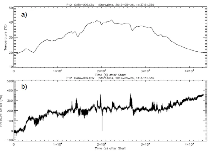
Fig. 7. Example data from a logger (“P12”) during a follow-up measurement campaign, showing about 12 h of data. (a) Sensor temperature

rises throughout the day to a peak (in the shade) of 40◦C. Note that dips in temperature occur at∼5000 s intervals. The timestamp on the

data files is Eastern Daylight Time (from the author’s laptop), which is 3 h ahead of local time (Pacific). Thus, the record shown here begins

at 08:38 a.m. LT (local time). (b) Pressure record, with an initial offset subtracted. Fluctuations of∼10 Pa are seen throughout, but some

isolated bursts of∼100 Pa noise are seen, correlating with the temperature dips; the instance at 27 000 s is shown in more detail in Fig. 8.

trials indicated above, some dramatically poorer behaviors were also noted. These have been studied here in order to improve them for future measurements, and in particular to improve the performance of automatic dust devil detection algorithms.

First, a sawtooth pattern (Fig. 8) was sometimes appar-ent in the data – corresponding to what looks like noise in the daily view (Fig. 7). This did not degrade the data qual-ity dramatically beyond the normal noise level for the two loggers that ran with 100 ms sample interval, but the third unit with a sample interval of 500 ms showed a much more pronounced sawtooth. Interestingly, the scatter in the data for that unit within each sawtooth cycle was noticeably smaller than for the other two, suggesting that perhaps the highest sample rate causes higher measurement noise. The sawtooth cycle was a very regular 100 samples, which was the arbi-trary value chosen as a compromise between the limited ex-pectation of utility of the temperature data and the data vol-ume cost of recording it. Thus, it was suspected upon ex-amination of the data that the temperature recording is actu-ally used in the temperature correction of the pressure sensor data, and that the sawtooth (most noticeable during the day) was due to comparatively rapid temperature changes such that the correction was not being correctly applied. An ob-vious mitigation strategy is to simply decrease the interval between temperature readings to just a few seconds (i.e., ev-ery 10th sample for a 500 ms pressure sampling cadence, or

every 50th for the fastest 100 ms). The improvement in data quality is likely worth the data volume penalty (see Sect. 2.2). Because this temperature calibration error is somewhat deter-ministic, a correction algorithm can be applied to improve the data quality (Fig. 8). Different filtering options (even simple smoothing) can likely improve the detectability of dust devil pressure drops, especially when the width of the drop be-ing sought is much (∼10×) wider than the interval between temperature corrections.

Another mitigation (Alex Kooney, personal communica-tion) is to add a “raw-output” flag to the configuration file; this option (not documented in the product manual, GCDC, 2010) forces the device to output a reading that is not “cor-rected” with an erroneous temperature. While this entails post-processing to recover absolute pressures, or indeed to correct for long-term relative variations, this raw output will vary smoothly without any sawtooth noise, which may be better for detecting short-term dips in pressure due to dust devils.

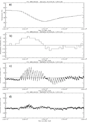
Fig. 8. The 2000 s of data from Fig. 6 showing (a) the temperature evolution (note 0.1◦C quantization) and (b) the temperature increment

between successive samples (acquired at 100 pressure-sample intervals, or 50 s). The pressure readings (c) show a∼100 Pa sawtooth noise

due to improper temperature correction – it is seen that the sawtooth amplitude and sign correlates rather well with the temperature derivative rate. (d) A post-processing correction algorithm subtracts a sawtooth correction (i.e., a cyclic ramp with a period of 50 s, synchronized to the temperature reading) with an amplitude proportional to the temperature derivative in (c): it is seen that the noise is reduced by a significant

factor (∼3–4) to∼20–30 Pa.

is in fact large enough to give a noticeable pressure error). Significant correction of this noise by post-hoc processing is likely to be challenging, since the information to make the correction simply does not exist (i.e., this noise is somewhat comparable with the residual noise after bad sawtooth has been corrected.) However, as for the sawtooth noise, chang-ing the temperature measurement cadence to a much longer,

or (desirably) much shorter, interval will mitigate its impact on dust devil detection.

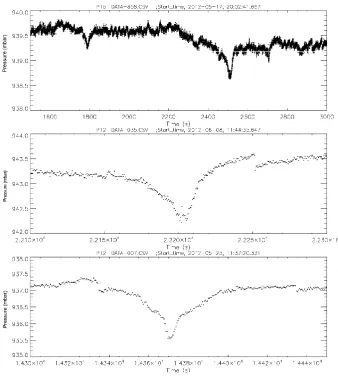
Fig. 9. Some example dust devil signatures. (a) An isolated 30s-wide event with a peak pressure drop of 0.5 mbar, (b) a narrow (∼30 s, 0.3 mbar) and 400 s later a wide (300 s, 0.5 mbar) feature, the latter presumably due to a large devil at some distance. (c) A sequential pair

of similarly-sized devils, each∼300 s wide and∼0.4 mbar deep and separated by 5000 s. Note each plot is scaled differently. Data are

uncorrected for sawtooth effects.

reject those lines (the text file can be manually edited, but this would become prohibitively laborious for large amounts of data such as that analyzed here). No obvious time or tempera-ture correlation has been noted with these dropouts (although notably one brief dropout occurs in the middle of a dust devil encounter – see later – suggesting that perhaps nearby elec-trostatic discharge associated with triboelectric effects in the dust can cause data transfer problems).

While these issues are inconvenient, especially to auto-mated processing of the data, it should be recognized that overall they occur fairly seldom. Many files are unaffected, and in most of those that are, over 99 % of lines in the ASCII record are uncorrupted.

While the noise in the data acquired in this initial field test was somewhat distracting due to the more rigorous temper-ature excursions experienced than is typical in laboratory or domestic settings, it was nonetheless easy to identify many

dust devil signatures by sight. Further, important lessons have been learned for the optimum settings to use for on-going and future measurements.

5 Example dust devils and other observations

A systematic investigation of dust devil population data from the logger described here will be perfomed in future work, using both human and machine methods to detect dust dev-ils. An initial (human) reconnaissance of the data show many “classic” dust devil encounters, and some examples are shown in Figs. 9–11.

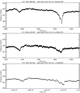
Fig. 10. Further dust devil signatures. (a) A 0.4 mbar 60 s event and a 0.6 mbar 100 s event, spaced by 700 s. (b) A 1 mbar event, 500 s long, with an apparent double dip in pressure, perhaps due to a core wandering in a cycloidal pattern (c) the largest event noted so far, 1.5 mbar deep, 100 s wide, with a distinct 0.6 mbar 10 s-wide core. Note each plot is scaled differently. Data are uncorrected for sawtooth effects.

the pre-encounter value). This was noted, e.g., by Sin-clair (1973), although only a handful of examples were shown.

Two of the plots show two dust devils; it is tempting to speculate these may be pairs (e.g., formed by the break of a horizontal roll vortex into two counter-rotating vertical vor-tices). Future work will explore, with the robust statistics per-mitted by the large dataset being acquired, the possibility of pairing or other temporal clustering.

Figure 10 shows additional examples. The second event in Fig. 10a is noticeably asymmetric, with a slow dip but a fast recovery. This could be the result of a change in wind speed involving a slow approach with a faster departure for a dust devil that has a constant intensity; or where, for instance, a dust devil suddenly “dies” soon after closest approach. Again, the methodology described in the present paper will permit enough data to be acquired to determine whether such asymmetry (again, noted first by Sinclair, 1973) is random

or whether, for example, the pressure decline on the lead-ing face of a devil is shallower than the traillead-ing side. This example also underscores the potential for future measure-ments with an array of loggers to resolve the temporal– spatial ambiguity.

The third example in Fig. 10 is the most intense encounter observed so far, 1.5mbar deep. Interestingly, it seems to have a distinct broad ramp on either side, a few tens of seconds wide, with a sharp central dip.

Fig. 11. A pair of dust devils, about 8 min apart, observed in all three loggers (shifted to show the coherence of the records). The bottom two

plots are essentially synchronous, but the first plot is about 90 s earlier in time. Note that the second devil is still detectable at the∼0.5 mbar

level in the last record (P16) despite the∼0.25 mb sawtooth noise (uncorrected in this plot). The second devil evidently passed closest to

the P10, where the pressure drop is both sharpest in structure and deepest (∼1.5 mbar); an 8.98 s gap exists in the data at 3469.496 s, in the

middle of the dust devil encounter, suggesting a possible electrostatic interference.

devils were more intense. Since the P15 dip appears deeper than P16, at least for the first devil, it seems likely that the devil passed closer to P15 than to P16.

Both dust devils, in all three records, appear to be asym-metric, with a slower dip and fast recovery. The possibility (discussed above) that this could be caused by “death” of the dust devil after P10 passage appears to be excluded in this in-stance in that an apparently correlated encounter with P15/16 occurs. A random encounter of a new devil appears unlikely. It is clear that multiple stations offer interesting prospects for array study, and even with only 3 stations important addi-tional information is obtained and can address ambiguities inherent in single-station records.

Note that there is some evidence of a dual dip in the second devil, perhaps indicating the core. Interestingly, the P16 record has a data gap here where no data was written (while data gaps do occur briefly when a new datafile is be-ing opened, in this instance the gap appears in the middle of a file). It is possible that some electrostatic discharge effect was responsible.

Fig. 12. Uncorrected pressure record over daylight hours. Beginning around 13 000 s (i.e., around local noon), an oscillation in pressure develops with a period of about 1000 s, and is seen most prominently at the middle of the center panel at around 14:00 LT when dust devil activity is near its peak. In this uncorrected data, the periodic pressure cycle is somewhat highlighted by the sawtooth due to correlated temperature changes.

6 Conclusions and future work

The unit investigated here is affordable enough ($ 120) to consider deploying in arrays to measure the two-dimensional structure of convection, or (with wider spacing) simply to increase the number of dust devil encounters obtained. The unit cost is modest enough compared with the costs of de-ployment that it can be considered partially expendable (i.e., some attrition of a deployed set can be tolerated with useful data still obtained).

The data storage capability of the units permits several months of data at a high sample rate (10 Hz) or a year or more at a lower rate. The default AA battery installation, however, permits less than a week at this rate. The power supply mod-ifications described in this paper enable much longer-term operation than the nominal configuration, and thus permit a larger amount of data to be acquired, permitting (for exam-ple) robust statistics over several months to be obtained from a single deployment in the field.

Our initial surveys highlighted that solar-powered in-stallations may suffer higher attrition than more covert

battery-powered units. Additionally, the importance of tem-perature correction of the pressure data is noted: specifically, the temperature of the sensor should be logged (and thus the correction updated) at a cadence different from the duration of events being searched for. Although a data volume penalty results, this cadence should be as high as possible, once a second or better. We have described, however, how data de-graded by less frequent (∼50 s) updates can be substantially recovered by post-processing.

periodicity/clustering, and an evaluation of the size statistics (Lorenz, 2012). Data from sensors such as these can be aug-mented by comparison with other meteorological variables such as wind speed.

Acknowledgements. This work was funded by NASA through the

Mars Fundamental Research Program. Brian Jackson, Pete Lana-gan and Jani Radebaugh are thanked for assistance in the field. I thank Alex Kooney of GCDC for useful correspondence regarding internal details of the dataloggers. I thank the several reviewers for their comments.

Edited by: A. Benedetto

References

Balme, M. and Greeley, R.: Dust devils on Earth and Mars, Rev. Geophys., 44, RG3003, doi:10.1029/2005RG000188, 2006. Bosch Sensortech: BMP-085 Digital Pressure Sensor, Product

Datasheet rev 1.2, Robert Bosch GmbH, Germany, 2009. Ellehoj, M. D., Gunnlaugsson, H. P., Taylor, P. A., Kahanpaa, H.,

Bean, K. M., Cantor, B. A., Gheynani, B. T., Drube, L., Fisher,

Lorenz, R. D., Jackson, B., and Barnes, J.: Inexpensive Timelapse Digital Cameras for Studying Transient Meteorological Phenom-ena: Dust Devils and Playa Flooding, J. Atmos. Ocean. Tech., 27, 246–256, 2010.

Murphy, J. and Nelli, S.: Mars Pathfinder convective vortices: frequency of occurrence, Geophys. Res. Lett., 29, 2103, doi:10.1029/2002GL015214, 2002.

Pathare, A. V., Balme, M. R., Metzger, S. M., Spiga, A., Towner, M. C., Renn`o, N. O., and Saca, F.: Assessing the power law hypoth-esis for the size-frequency distribution of terrestrial and Martian dust devils, Icarus, 209, 851–852, 2010.

Renno, N. O., Abreu, V. J., Koch, J., Smith, P. H., Hartogensis, O. K., De Bruin, H. A. R., Burose, D., Delory, G. T., Far-rell, W. M., Watts, C. J., Garatuza, J., Parker, M., and Car-swell, A.: MATADOR 2002: A pilot field experiment on con-vective plumes and dust devils, J. Geophys. Res., 109, E07001, doi:10.1029/2003JE002219, 2004.

Ryan, J. A. and Lucich, R. D.: Possible Dust Devils, Vortices on Mars, J. Geophys. Res., 88, 11005–11011, 1983.

Sinclair, P. C.: The Lower Structure of Dust Devils, J. Atmos. Sci., 30, 1599–1619, 1973.