Performance Analysis and Optimization of Parallel Scientific Applications on CMP Clusters

Volume 10, Number 1, pp. 61–74. http://www.scpe.org c 2009 SCPE

PERFORMANCE ANALYSIS AND OPTIMIZATION OF PARALLEL SCIENTIFIC APPLICATIONS ON CMP CLUSTERS

XINGFU WU, VALERIE TAYLOR, CHARLES LIVELY ANDSAMEH SHARKAWI∗

Abstract. Chip multiprocessors (CMP) are widely used for high performance computing. Further, these CMPs are being configured in a hierarchical manner to compose a node in a cluster system. A major challenge to be addressed is efficient use of such cluster systems for large-scale scientific applications. In this paper, we quantify the performance gap resulting from using different number of processors per node; this information is used to provide a baseline for the amount of optimization needed when using all processors per node on CMP clusters. We conduct detailed performance analysis to identify how applications can be modified to efficiently utilize all processors per node using three scientific applications: a 3D particle-in-cell, magnetic fusion application Gyrokinetic Toroidal Code (GTC), a Lattice Boltzmann Method for simulating fluid dynamics (LBM), and an advanced Eulerian gyrokinetic-Maxwell equation solver for simulating microturbulent transport in plasma (GYRO). In terms of refinements, we use conventional techniques such as loop blocking, loop unrolling and loop fusion, and develop hybrid methods for optimizing MPI Allreduce and MPI Reduce. Using these optimizations, the application performance for utilizing all processors per node was improved by up to 18.97% for GTC, 15.77% for LBM and 12.29% for GYRO on up to 2048 total processors on the CMP clusters.

Key words: performance analysis, performance optimization, chip multiprocessors (CMP), clusters, parallel scientific appli-cations

1. Introduction. The current trend in high performance computing systems has been shifting towards cluster systems with CMPs (chip multiprocessors). Further, the CMPs are usually configured hierarchically (e.g., multiple CMPs compose a multi-chip module and multiple multi-chip modules compose a node) to compose a node of a CMP cluster. For example, each node of DataStar P690 at the San Diego Supercomputing Center (SDSC) consists of four multi-chip modules for which each module consists of four CMPs, and each CMP consists of two cores [13]. SDSC DataStar p655 has one multi-chip module per node. When using these clusters to execute a given application, one issue to be addressed is how to efficiently utilize all processors per node given the significant sharing of node resources (e.g., caches, networks) among the processors within the node. In this paper, we quantify the performance gap resulting from using different number of processors per node for application executions. Further, we use the detailed performance results to identify performance optimizations that can be made to these applications for efficient execution using all processors per node.

Other work in this area has focused on using all processors per node. Phillips et al. [10] presented the performance results for 4 processors per node and 3 processors per node on Lemieux Alpha cluster at Pittsburgh Supercomputing Center that has a maximum of 4 processors per node, and noted that leaving idle one processor per node reduces performance variability. Petrini et al. [9] found that application execution times may vary significantly between 3 processors per node and 4 processors per node on a large scale supercomputer, ASCI Q. They concluded that system noise within the nodes was the source of the performance variability, and used a discrete-event simulator to evaluate the contribution of each component of the noise to the overall application behavior. In our previous work [20], we quantified the performance gap resulting from using different number of processors per node for the NAS parallel benchmarks on SMP clusters. In this paper, however, we identify optimizations that result in efficient use of all processors per node on the CMP clusters for large-scale scientific applications.

The three large-scale, scientific applications used for our experimental analysis are as follows: a 3D particle-in-cell application Gyrokinetic Toroidal Code (GTC) in magnetic fusion [2], a Lattice-Boltzmann Method for simulating fluid dynamics (LBM) [19], and an advanced Eulerian gyrokinetic-Maxwell equation solver for simulating microturbulent transport in core plasma (GYRO) [3]. The Prophesy system [17, 16] is used to collect all application performance data. The programming environments and problem sizes used in the three applications are shown in Table 1.1. The test case studied for GTC is 100 particles per cell and 100 time steps. The problem size for LBM is a 3D mesh computational domain. B1-std and B2-cy are two benchmark datasets for GYRO.

The experiments conducted in this work utilize systems with different number of processors per node. DataStar P655 has 8 processors per node and P690 has 32 processors per node. Bassi has 8 processors per node and Seaborg has 16 processors per node at the DOE National Energy Research Scientific Computing Center

∗_{Department of Computer Science, Texas A&M University, College Station, TX 77843, USA ({wuxf, taylor}@cs.tamu.edu)}

Table 1.1

Programming environments and problem sizes of GTC, LBM and GYRO

Application Discipline Problem Sizes Programming Environments GTC Magnetic Fusion 100 particles per cell Fortran90, MPI, OpenMP

LBM Fluid Dynamics 128x128x128 C, MPI

512x512x512

GYRO Plasma Physics B1-std: 6x140x4x4x8x6 Fortran90, MPI B2-cy: 6x128x4x4x8x6

(NERSC) [8]. BlueGene/L at the Renaissance Computing Institute has 2 processors per node [11]. Further, each system has a different node memory hierarchy. The experimental results indicate that large performance gaps can exist. For example, the performance gap for LBM using 32 processors corresponds to an increase of 23.53% when using 32 processors per node versus using 8 processors per node (resulting from resource conflicts) for a problem size of 128x128x128 on the P690.

Much of the computation involved in parallel scientific applications occurs within nested loops. Therefore, loop optimization is fundamentally important for these applications. In this paper, we use loop blocking, loop unrolling and loop fusion to optimize three scientific applications. We also develop hybrid methods to optimize MPI Allreduce and MPI Reduce, which are very common communication subroutines. For a given optimization of GTC, the application performance was improved by up to 18.97% on up to 2048 processors. For a given optimization of LBM, the application performance was improved by up to 15.77% when utilizing all processors per node. For a given optimization of GYRO, the application performance was improved by up to 12.29% when utilizing all processors per node. This is important because with CMP clusters, the only way to access a large number of processors is to use all processors per node.

The remainder of this paper is organized as follows. Section 2 discusses the architecture and memory hierarchy of the five supercomputers used in our experiments, and presents their MPI performance when utilizing different configurations of the node hierarchy. Section 3 discusses application optimization methods used to refine the applications. Section 4 investigates performance characteristics of GTC, and presents our optimization results. Section 5 discusses performance characteristics and optimization results of LBM. Section 6 explores performance characteristics and optimization results of GYRO. Section 7 concludes this paper. In the remainder of this paper, we describe a processor partitioning scheme asMxN whereby M denotes the number nodes with N processors per node (PPN). The job scheduler for each supercomputer always dispatches one process to one processor. All experiments were executed multiple times to insure consistency of the performance data.

2. Execution Platforms and Corresponding MPI Performance. Details about the five supercom-puters used for our experiments are given in Table 2.1. These systems differ in the following main features: number of processors per node, configurations of node memory hierarchy, CPU speed, multi-core processors, and communication networks.

DataStar P655 [13] has 176 (8-way) compute nodes with 1.5GHz POWER4 and 16GB memory, and 96 (8-way) compute nodes with 1.7GHz POWER4 and 32GB memory. Each node of P655 has one MCM (Multiple-Chip Module) with 4 chips per MCM. DataStar P690 has 7 (32-way) compute nodes. Each node of P690 has four MCMs with 4 chips per MCM. The use of 8-way nodes for P655 is exclusive. The use of 32-way nodes on P690 is shared among users, and the access to P690 is limited to at most five nodes.

UNC RENCI BlueGene/L [11] is a system-on-chip supercomputer, and is designed to achieve high perfor-mance for low cost and with low power consumption. The BlueGene/L has 1024 dual 700 MHz PowerPC 440 nodes with 1GB memory per node. Note that L2 cache is a prefetch buffer that holds 16 128-byte lines.

Table 2.1

Specifications of five supercomputer architectures

Configurations P655 BlueGene/L P690 Seaborg Bassi

Number of Nodes 272 1024 7 380 111

MCMs/Node 1 NA 4 NA NA

chips/MCM 4 NA 4 NA NA

Cores/chip 2 2 2 1 1

CPUs/Node 8 2 32 16 8

CPU type 1.5,1.7GHz 700 MHz 1.7GHz 375MHz 1.9GHz

POWER4 PowerPC POWER4 POWER3 POWER5

Memory/Node 16,32GB 1GB 128GB 16-64GB 32GB

L1 Cache/CPU 64/32 KB 32KB 64/32 KB 32/64 KB 64/32 KB L2 Cache/chip 1.41MB 128-byte lines 1.41MB 8MB 1.92MB

L3 Cache/chip 32MB 4MB 32MB NA 36MB

Network Federation 3D Torus Federation Colony Federation

2.1. Multi-Chip Module and Processor Affinity. In this section, we address processor affinity (i. e., how processes are dispatched to processors) and its policy in the following CMP clusters: P655, P690, and BlueGene/L. Although Bassi is POWER5 system, it is configured with only one active core per POWER5 chip. Seaborg is a POWER3 system with one processor per chip.

Fig. 2.1.A logical view of a MCM [1]

Fig. 2.1 shows the logical view of a POWER4 MCM. The MCM is used as an eight-way basic building block. Each MCM has four POWER4 chips; the two processors on the same chip share L2 and L3 caches. The logical interconnection of four POWER4 chips is point-to-point with uni-directional buses connecting each pair of chips to form an 8-way SMP with an all-to-all interconnection topology. P655 has one MCM per node. With the single MCM configuration, each chip always sends requests, commands and data on its own bus, but snoops all buses for requests or commands from other MCMs. Multiple MCMs can be interconnected to form larger SMPs, such as P690 with four MCMs, by extending each bus from each module to its neighboring module in one direction.

The processor affinity policy for POWER4 and POWER5 is discussed in [4]. When a virtual processor is dispatched, it is first dispatched onto the same physical processor that it last ran on. Otherwise, it will be dispatched onto the first available processor in the following order: on the same chip, then to another chip on the same MCM, then to a chip on the same node.

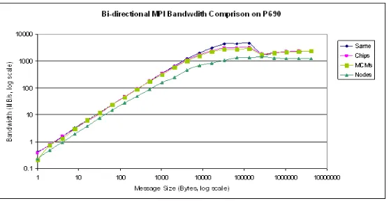
Fig. 2.2.Bi-directional bandwidth comparison on P690 using processor binding

3. Application Optimization Methods.

3.1. Loop Optimizations. Much of the computation involved in scientific applications such as LBM, GTC and GYRO occurs within nested loops. Therefore, loop optimization is fundamentally important for such applications. In this section, we discuss loop blocking, loop unrolling and loop fusion to optimize the scientific applications.

Loop blocking is a well-known loop optimization technique to aid in taking advantage of memory hierarchy; its main purpose is to eliminate as many cache misses as possible. This technique transforms the memory domain of an application into smaller chunks, such that computations are executed on the chucks that easily fit into cache to maximize data reuse. The optimal loop block size varies with different applications on different systems. In this paper, we apply the following loop block sizes: 2x2, 4x4, 8x8 and 16x16 to the three scientific applications to measure which loop block size is optimal. Our experimental results indicate that the optimal loop block size is 2x2 on BlueGene/L and 4x4 on P655 for GTC, and 16x16 on BlueGene/L and 4x4 on P655 for LBM and GYRO.

Loop unrolling is a well-known code transformation technique that replicates the original loop body multiple times, adjusts the loop termination code and eliminates redundant branch instructions. Outer loop unrolling can increase computational intensity and minimize load/stores, while inner loop unrolling can reduce data dependency and eliminate intermediate loads and stores. We combine inner and outer loop unrolling to optimize the scientific applications. For examples, we unroll the inner loops four times for four major double nested loops in GTC code so that we reconfigure the double nested loops into the single loops, then use compiler directives for further loop unrolling.

The performance for the hand-tuned scientific codes using loop blocking and unrolling can be further improved by using compiler directives, which are hardware-specific. The IBM XL Fortran compiler provides some hardware-specific directives for performance optimization, such as –qdirective=UNROLL AND FUSE [4]. The UNROLL AND FUSE directive instructs the compiler to allow loop unrolling and fusion where applicable. Loop fusion is also a code transformation technique. It minimizes the required number of loop iterations, and improves data locality by increasing data reuse in registers and cache. For each execution environment used in this study, we utilize the appropriate compiler directives to further optimize the code.

3.2. Hybrid Methods for MPI Allreduce and MPI Reduce. In this section, we present our hybrid methods to optimize MPI Allreduce and MPI Re-duce, which are common in GTC and GYRO. In scientific applications, especially GTC and GYRO, MPI Allreduce dominates the most communication time. In order to optimize MPI Allreduce, we incorporate the following hybrid method that we implemented:

• Use Intel’s MPI benchmarks to measure the performance of the original MPI Allreduce with different message sizes on each cluster,

• Measure the performance of Rabenseifner’s algorithm for allreduce in [14] with different message sizes on the same cluster,

• Compare both performance to decide message size ranges for the best performance,

Table 4.1

Datasets with scaling the number of processors for GTC

Processors 2 4 8 16 32 64 128 256 512 1024 2048

micell 100 100 100 100 100 100 200 400 800 1600 3200 mecell 100 100 100 100 100 100 200 400 800 1600 3200

mzetamax 2 4 8 16 32 64 64 64 64 64 64

npartdom 1 1 1 1 1 1 2 4 8 16 32

Rabenseifner’s algorithm performs a reduce-scatter followed by an allgather for MPI Allreduce, and the algorithm also performs a reduce-scatter followed by a gather for MPI Reduce. The hybrid method takes different systems and message sizes into account in order to optimize MPI Allreduce. We also use the similar hybrid method to optimize MPI Reduce. A MPI program is required to be recompiled with our own MPI library for the two subroutines Allreduce and Reduce.

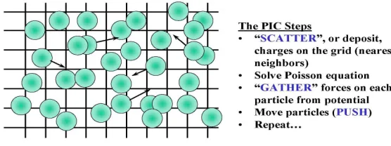
4. Gyrokinetic Toroidal Code (GTC). The Gyrokinetic Toroidal code (GTC) [2] is a 3D particle-in-cell application developed at the Princeton Plasma Physics Laboratory to study turbulent transport in magnetic fusion. GTC is currently the flagship SciDAC fusion microturbulence code written in Frotran90, MPI and OpenMP. Fig. 4.1 shows a visualization of potential contours of microturbulence for a magnetically confined plasma using GTC. The finger-like perturbations (streamers) stretch along the weak field side of the poloidal plane as they follow the magnetic field lines around the torus [12]. Fig. 4.2 presents the basic steps in the GTC code.

Fig. 4.1.Potential contours of microturbulence for a magnetically confined plasma [12]

Fig. 4.2.Particles in cell (PIC) steps [2]

The test case for GTC studied in this paper is 100 particles per cell and 100 time steps. The problem sizes for the GTC code are listed in Table 4.1, where micell is the number of ions per grid cell, mecell is the number of electrons per grid cell, mzetamax is the total number of toroidal grid points, and npartdom is the number of particle domain partitions per toroidal domain.

Table 4.2

Performance comparisons of GTC on 2 processors on P655

Across 2 nodes Across 2 chips Within a chip

Metrics 2x1/1PPC 1x2/1PPC 1x2/2PPC

Runtime (% difference) 984.26 (baseline) 990.02 (0.59%) 1114.32 (13.21%)

L1 hit rate 92.356% 92.375% 92.386%

TLB miss rate 0.005% 0.005% 0.005%

L2 bandwidth/processor 4618.906MB/s 4582.185MB/s 4071.585MB/s

% accesses from L2 2.228% 2.214% 2.235%

Table 4.3

Performance comparisons of GTC on 2 processors on P690

Across 2 nodes Across 2 MCMs Across 2 chips Within a chip Metrics 2x1/1PPM-1PPC 1x2/1PPM-1PPC 1x2/2PPM-1PPC 1x2/2PPM-2PPC

Runtime 980.23 994.58 1001.49 1009.66

(% difference) (baseline) (1.46%) (2.17%) (3.00%)

L1 hit rate 92.515% 92.48% 92.457% 92.475%

TLB miss rate 0.005% 0.005% 0.005% 0.005%

L2 bandwidth 4578.505 MB/s 4499.834 MB/s 4491.888 MB/s 4457.119 MB/s /processor

% accesses 2.211% 2.181% 2.177% 2.16%

from L2

to the baseline configuration corresponding to using one processor per node (or the least amount of sharing of node resources). There is 13.21% increase in execution time when using two processors within the same chip (1x2/2PPC) due to contention resulting from the sharing of resources, such as L2 and L3 caches. For the case of using one processor per chip with two chips in the same MCM (1x2/1PPC), there is a very small increase in execution time (only 0.59%). Recall that each node on P655 has one MCM, which consists of four dual-core POWER4 chips. Table 4.2 also presents the hardware counters’ performance using hpmcount [5]. The hardware counters indicate large difference (11.85%) in L2 bandwidth per processor for the two cases of using one processor per node versus using two processors within the same chip. Hence, there is significant contention for L2 when using two processors within the same chip.

Table 4.3 shows the performance results for dispatching two processes to two processors on the same chip, on two different chips on the same MCM, or two different chips on two different MCMs on P690 for two processors, respectively. Each node on P690 has four MCMs with four dual-core POWER4 chips per MCM shown in Table 2.1. There is only a 3.00% increase in execution time when using two processors within the same chip (1x2/2PPC) due to contention resulting from the sharing of resources, such as L2 and L3 caches. Comparing Table 4.3 with Table 4.2, it is clear that L2 bandwidth per processor accounts for the performance difference when using two processors within one chip (1x2/2PPC) versus using two processors across nodes (2x1/1PPM-1PPC).

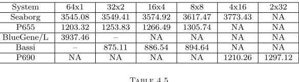
Table 4.4 indicates the performance gaps resulting from using different PPN on a total of 64 processors on five supercomputers. As expected, the smallest times corresponds to the minimum amount of sharing of node resources. With increasing number of PPN, the application execution time increases. The performance data in Table 4.4 utilized default processor affinity described in Section 2.1. For example, with the 16x4 configuration on P655 (16 nodes with 4 PPN), the 4 processors per node were dispatched such that the only two chips were used, whereby both cores per chip were used. The time difference between the schemes 64x1 and 8x8 is 8.51% on P655. The time difference between the schemes 64x1 and 4x16 is 6.44% on Seaborg. The time difference between the schemes 32x2 and 8x8 is 2.23% on Bassi. The time difference between the schemes 4x16 and 2x32 is 7.18% on P690. Because the GTC code could not be executed on UNC RENCI BlueGene/L with 2 PPN (in VN mode) except 2048 processors, we could not collect any data for using 2 PPN on the machine. We find that the subroutinespushi andchargei in GTC take more than 90% of the application execution time on 64 processors, and are sensitive to different memory access patterns and communication patterns for different PPN.

Table 4.4

Execution times (seconds) of GTC for different PPN on 64 processors

System 64x1 32x2 16x4 8x8 4x16 2x32

Seaborg 3545.08 3549.41 3574.92 3617.47 3773.43 NA P655 1203.32 1253.83 1266.49 1305.74 NA NA

BlueGene/L 3937.46 – NA NA NA NA

Bassi – 875.11 886.54 894.64 NA NA

P690 NA NA NA NA 1210.26 1297.12

Table 4.5

Performance comparisons of GTC on P655 using processor binding

32x2 16x4

2PPC 1PPC % difference 2PPC 1PPC % difference 1253.83 1218.31 2.92 1266.49 1230.47 2.93

4.2. Application Performance Optimization. Much of the computation involved in GTC, especially the subroutinespushi andchargei, occurs within nested loops. Therefore, we use loop blocking, loop unrolling and loop fusion to optimize the application. We also use the hybrid method for MPI Allreduce to optimize MPI Allreduce. Further, MPI Allreduce dominates the most communication time of the code on large number of processors. Therefore, we use the hybrid method described in Section 3 to optimize the MPI Allreduce. The range of message sizes are defined on different systems as follows: for P655, the hybrid method uses the original algorithm for the message sizes of less than 1KB and the Rabenseifner’s algorithm otherwise. For BlueGene/L, because GTC could only be executed on the number of processors with 1PPN, the hybrid method uses the Rabenseifner’s algorithm for the message sizes of between 256 bytes and 2KB and the original algorithm otherwise.

Our experimental results indicate that the optimal loop block size for GTC is 2x2. This block size is used to optimize outer loops of the triple nested loops in GTC code. We also unroll the inner loops four times for four major double nested loops in the subroutines pushi and chargei such that the double nested loops are reconfigured into single loops. Further, we used the compiler options consistent with that given in [2].

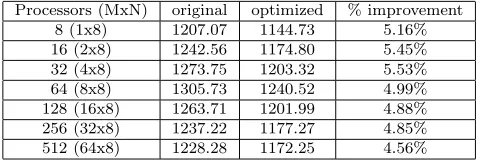
The results of applying the aforementioned optimizations are given in Tables 4.6 and 4.7 for BlueGene/L and P655, respectively. We performed the optimization in series so that we could quantify the results of each optimization. These results are not given in this paper due to space. The results, however, indicated that majority of the optimization for GTC resulted from hand-tuned loop unrolling and blocking. We achieve up to 18.97% performance improvement on BlueGene/L. It should be noted that the performance gap for P655 using 64x1 versus 8x8 was 8.51% in Table 4.4. Using the aforementioned optimizations we were able to reduce the execution time for using all PPN by 4.99%.

5. LBM Application. The Lattice Boltzmann Method (LBM) [19] is widely used for simulating fluid dynamics; this method has the ability to deal efficiently with complex geometries and topologies. The LBM application is computation intensive. In our simulations, we use the D3Q19 lattice model (19 velocities in 3D) with the collision and streaming operations. The LBM application code is divided into six kernels, which are given below in Fig. 5.1.

Table 4.6

Execution time (seconds) comparison of GTC between the original and the optimized on BlueGene/L

Processors (MxN) original optimized % improvement 8 (8x1) 3804.03 3082.54 18.97% 16 (16x1) 3834.98 3124.80 18.52% 32 (32x1) 3869.60 3166.56 18.17% 64 (64x1) 3937.46 3221.31 18.19% 128 (128x1) 3919.06 3202.81 18.28% 256 (256x1) 3913.07 3208.95 17.99% 512 (512x1) 3820.28 3120.65 18.31% 1024 (1024x1) 3788.49 3096.36 18.27% 2048 (1024x2) 3808.03 3108.40 18.37%

Table 4.7

Execution time (seconds) comparison of GTC between the original and the optimized on P655

Processors (MxN) original optimized % improvement 8 (1x8) 1207.07 1144.73 5.16% 16 (2x8) 1242.56 1174.80 5.45% 32 (4x8) 1273.75 1203.32 5.53% 64 (8x8) 1305.73 1240.52 4.99% 128 (16x8) 1263.71 1201.99 4.88% 256 (32x8) 1237.22 1177.27 4.85% 512 (64x8) 1228.28 1172.25 4.56%

The description of each kernel is given below:

• Initialization: reads input files and sets up the initial parameter values.

• Collision: computes the effect of the collisions, which occur during the particle movement. • Communication: is to communicate the needed data among neighboring blocks.

• Streaming: moves particles in motion to new locations along their respective velocities.

• Physical: calculates macroscopic variables such as fluid density, which are used in the collision and streaming steps.

• Finalization: cleans up the program after everything is done, and outputs the results.

The kernelsCollision, Communication, Streaming, andPhysical stay in a loop with the number of iterations of 200. The kernelsInitialization andFinalizationare executed once. The problem size for the LBM application is a 3D mesh computational domain. In this paper, we use two problem sizes of 128x128x128 and 512x512x512 for the LBM application in our experiments.

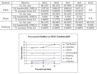
5.1. Application Performance Analysis. Table 5.1 provides the execution times of the LBM application with problem sizes of 128x128x128 and 512x512x512 for different PPN on a total of 32 processors across the five supercomputers. The performance data was collected using the default processor affinity described in Section 2.1. With increasing number of PPN, the application execution time increases significantly on Seaborg, P655, and P690; there is very little difference in execution times on Bassi. For example, the time difference between 1 PPN and 16 PPN on Seaborg is 21.3% for the problem size of 512x512x512, and 15.83% for the problem size of 128x128x128. The time difference between the scheme 1 PPN and 8 PPN on P655 is 20.73% for the problem size of 512x512x512, and 10.03% for the problem size of 128x128x128. The time difference between the scheme 8 PPN and 32 PPN on P690 is 17.79% for the problem size of 512x512x512, and 23.53% for the problem size of 128x128x128.

Table 5.2 indicates the results from using processor such that only one core per chip is used thereby minimizing resource sharing. The results indicate a 4.71% decrease in execution time for the 16x2 configuration and a 6.75% reduction in execution time for the 8x4 configuration. This indicates that processor binding can aid task schedulers in maximizing the application performance in dedicated usage of CMP nodes.

Table 5.1

Execution times (seconds) of LBM for different PPN on 32 processors

System Name Problem size 32x1 16x2 8x4 4x8 2x16 1x32

Seaborg 128x128x128_{512x512x512 6247.87}94.21 _6307.4194.42 _6418.7795.29 _6722.3198.72 _7578.84109.12 NA_NA

P655 128x128x128_{512x512x512 2154.94}33.09 _2224.7633.38 _2361.6734.57 _2601.6636.41 NA_NA NA_NA

P690 128x128x128_512x512x512 NA_NA NA_NA NA_{NA 2198.90}29.15 _2248.6230.35 _2590.1836.01

Bassi 128x128x128_{512x512x512 1379.63}21.43 _1382.3021.92 _1380.3221.14 _1384.8421.78 NA_NA NA_NA

BlueGene/L 128x128x128_{512x512x512 2252.99}33.40 _2253.2733.42 NA_NA NA_NA NA_NA NA_NA

Table 5.2

Performance comparisons of LBM on P655 using processor binding

16x2 8x4

2PPC 1PPC % difference 2PPC 1PPC % difference 2224.76 2124.66 4.71 2361.67 2212.28 6.75

for the L2 bandwidth. For example, the L2 bandwidth for the 32x1 scheme is more than 11% larger than that for the 4x8 scheme. On Bassi, there is very small difference in percentage accesses from L2 across different PPN due to 20GB large page size, which uses hardware prefetch mechanisms to eliminate costly TLB misses. Further, Bassi has the highest memory bandwidth and MPI bandwidth, which result in very little change in communication rate for the different configurations. Hence, the execution time is flat for the different PPN on Bassi. It is interesting that Bassi has the lowest L1 hit rate and correspondingly, the highest percentage accesses from L2.

5.2. Application Performance Characteristics and Optimization. In this section, we use the LBM application with the problem sizes of 128x128x128 and 512x512x512 to utilize the information learned from the previous section to determine how to optimize the application.

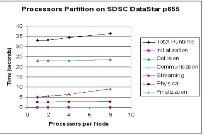
Fig. 5.2.Execution times of LBM for different PPN on 32 processors on P655

Table 5.3

Memory performance for LBM with the size of 512x512x512

System Metrics 32x1 16x2 8x4 4x8 2x16

P655

L1 hit rate 98.13% 98.15% 97.99% 97.69%

NA L2 bandwidth (MB/s) 1127.01 1098.07 1082.61 1015.14

% accesses from L2 0.618% 0.602% 0.593% 0.541%

Bassi

L1 hit rate 94.93% 92.82% 95.33% 95.85%

NA L2 bandwidth (MB/s) 3.035 4.788 2.523 2.145

% accesses from L2 5.069% 7.177% 4.669% 4.147%

Seaborg

L1 hit rate 99.14% 99.00% 98.93% 98.88% 99.14% L2 bandwidth (MB/s) 0.069 0.066 0.064 0.060 0.050

% accesses from L2 0.332% 0.380% 0.409% 0.420% 0.340%

Fig. 5.3.Execution times of LBM for different PPN on 32 processors on P690

Figs. 5.2, 5.3 and 5.4 also indicate how the LBM code and its kernels are sensitive to different memory access patterns and communication patterns on the CMP clusters. This kind of performance characteristics of the LBM code could not be found in most application performance analysis just based on a single run on a given number of processors. The kernelcollision dominates most of the application execution time, but the performance trend for the kernelStreaming is similar to that for the total runtime on P655. Optimizing the kernel collision does not eliminate the performance impact using different number of PPN. Hence, we focus on optimizing Streaming, which entails moving particles in motion to new locations along their respective 19 velocities [19]. This kernel requires a significant number of memory copy operations, which causes memory congestion when large numbers of PPN are used. In particular, Streaming consists of five triple-nested loops. We focus on using loop blocking to optimize the outer two loops of each triple-nested loop. For the sake of simplicity, we just present results for the large problem size of 512x512x512.

Table 5.4

Execution time (seconds) comparison of LBM between the original and the optimized on P655

Processors (MxN) original optimized % improvement Optimal block size

32 (4x8) 2601.66 2191.28 15.77% 4x4

64 (8x8) 1306.55 1110.71 14.99% 4x4

128 (16x8) 653.31 561.56 14.04% 4x4

256 (32x8) 319.71 287.71 10.01% 4x4

512 (64x8) 163.44 157.53 3.62% 16x16

1024 (128x8) 83.9 79.37 5.40% 16x16

2048 (256x8) 48.56 45.3 6.71% 16x16

Fig. 5.4. Execution times of LBM for different PPN on 32 processors on Seaborg

4x8, our optimization reduces execution time by 15.77%. This is a big improvement. Note that the performance improvement percentage trend decreases with increasing the number of total processors for the optimal block size of 4x4 because of the decrease of workload per processor and the increase of the communication percentage with increasing the number of processors. For the problem size of 512x512x512, the LBM application can only be executed on 32 processors or more because of the large sufficient memory requirement.

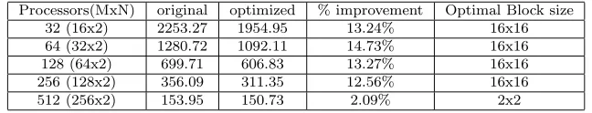
Table 5.5

Execution time (seconds) comparison of LBM between the original and the optimized on BlueGene/L

Processors(MxN) original optimized % improvement Optimal Block size

32 (16x2) 2253.27 1954.95 13.24% 16x16

64 (32x2) 1280.72 1092.11 14.73% 16x16

128 (64x2) 699.71 606.83 13.27% 16x16

256 (128x2) 356.09 311.35 12.56% 16x16

512 (256x2) 153.95 150.73 2.09% 2x2

Table 5.5 provides the performance comparison between the original code and the optimized for the problem size of 512x512x512 on RENCI BlueGene/L using all PPN. The optimized code with the block size of 16x16 achieved the best performance on 32, 64, 128 and 256 processors, but the optimized code with the block size of 2x2 obtained the best performance on 512 processors. For only optimizing the kernelStreaming in the original application code, the percentage of performance improvement is up to 14.73%. Compare to the results for different PPN on BlueGene/L in Table 5.1, this is a big improvement.

Hence, for the same problem size and same total number of processors, the loop blocking optimization resulted in much larger performance improvement of the LBM application when using all the processors per node versus one processor per node.

6. GYRO Application. GYRO [3] is an advanced Eulerian gyrokinetic-Maxwell equation solver that is capable of facilitating a better understanding of plasma microinstabilities and turbulence flow in the tokamak geometry. GYRO is used widely in simulating microturbulent transport in core plasma. In this section, we use GYRO with two benchmark datasets: the Waltz Standard benchmark, B1-std, consisting of grids of size 6 x 140 x 4 x 4 x 8 x 6, and the Cyclone Base Benchmark, B2-cy, consisting of grids of size 6 x 128 x 4x 4 x 8 x 6.

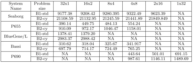
6.1. Application Performance Analysis. Table 6.1 provides the execution times of the GYRO appli-cation with B1-std and B2-cy for different PPN on a total of 32 processors. The performance data was collected using the default processor affinity described in Section 2.1. With increasing number of PPN, the application execution time increases significantly on Seaborg, P655, P690, and Bassi. For example, for the problem size of B1-std, there is a 55.79% increase in the execution time with increasing the PPN from 8 to 32 on P690, 42% increase in the execution time with increasing the PPN from 1 to 8 on P655, 9.15% increase with increasing the PPN from 1 to 8 on Bassi, and 4.86% increase with increasing the PPN from 1 to 16 on Seaborg.

Table 6.1

Execution times (seconds) of GYRO for schemes on 32 processors

System Problem 32x1 16x2 8x4 4x8 2x16 1x32

Name size

Seaborg B1-std 9177.38 9208.42 9280.395 9322.49 9623.39 NA B2-cy 21108.59 21132.95 21245.59 21441.89 21849.849 NA

P655 B1-std 390.14 449.75 484.13 554.24 NA NA

B2-cy 910.09 972.17 1046.47 1158.01 NA NA

BlueGene/L B1-std 1378.41 1379.20 NA NA NA NA

B2-cy 2983.37 2988.42 NA NA NA NA

Bassi B1-std 310.62 318.04 325.67 341.917 NA NA

B2-cy 697.79 714.17 724.49 765.25 NA NA

P690 B1-std_B2-cy NA_NA NA_NA NA_NA 443.64_{987.61 1146.11}501.01 _1489.69691.15

MPI Alltoall and MPI Allreduce subroutines account for more than 95% of the total communication across all platforms. It is noted that the performance of these routines are highly inefficient for using all PPN on P655, and the communication rate increases from 8.52% to 11.33% with increasing the PPN. We find that kernel 3 which computes the RHS of the electron and ion GKEs for both periodic and nonperiodic boundary conditions, andkernel 5 which computes the newly needed RHS in GYRO, dominate the application execution time, and are sensitive to memory access patterns and communication patterns for different processors per node.

Table 6.2

Performance comparisons of GYRO on P655 using processor binding

16x2 8x4

2PPC 1PPC % difference 2PPC 1PPC % difference 449.75 423.36 5.89 484.13 449.48 7.16

Table 6.2 indicates that using processor binding can achieve the better results for the 16x2 and 8x4 schemes. Using one processor per chips results in a 5.89% decrease in execution time for the 16x2 configuration and a 7.16% decrease in execution for the 8x4 configuration. This indicates that processor binding can aid task schedulers in maximizing the application performance in dedicated usage of CMP nodes.

6.2. Application Performance Optimization. In this section, we use the GYRO application with the problem size of B1-std to utilize the information learned from the previous performance analysis to determine how to optimize the application. It is noted that similar results occur for the problem size of B2-std.

Given the results of the application characterization and the kernel performance, we focus on optimizing the MPI Allreduce implementation to take advantage of the CMP clusters. In particular, we consider the communication architectures and message sizes to develop an adaptive communication pattern to optimize the MPI Allreduce. Such improvements impact kernels 3 and 5. The results shown in Table 6.3 illustrate the improvements that have been achieved utilizing a hybrid implementation of the MPI Allreduce routine for different message size ranges. The message size ranges for MPI Allreduce are defined on P655 as follows: the hybrid method uses the original algorithm for the message sizes of less than 1KB and the Rabenseifner’s algorithm otherwise. This optimization also consists of loop blocking the outer nested loops of the get RHS subroutine used inkernel 3 andkernel 5 with the optimal block size of 4x4. The compiler optimization utilizing the UNROLL AND FUSE option is applied to the entire code.

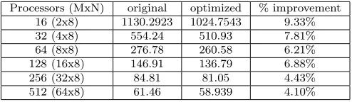
It is noted that the performance improvements in Table 6.3 are representative of an optimization on a small segment of the GYRO code, with respect to the get RHS subroutine. The results indicate performance improvement up to 9.33% on P655 and up to 12.29% on BlueGene/L. It is noted that, however, from Table 6.1 a performance difference of 42% on B1-std when increasing the PPN from 1 to 8 on P655 using a total of 32 processors. In Table 6.3, however, the performance improvement is 7.81%. The performance improvement is very good when we consider that only part of the GYRO code,kernels 3 and 5, were optimized. Further, only about one third of each of these two kernels was optimized. The improvement illustrates proof of concept. To achieve close to the 42% performance gap, we need to optimize the entire GYRO code.

the UNROLL AND FUSE option shown in Table 6.4. Note that the MPI Alltoall routine did not significantly impact the performance on the BlueGene/L system. The message size ranges for MPI Allreduce are defined on BlueGene/L: the hybrid method uses the original algorithm for the message sizes of less than 256 bytes and the Rabenseifner’s algorithm otherwise.

Note that the performance improvement percentage trend decreases with increasing the number of processors in Tables 6.3 and 6.4 because of the decrease of workload per processor and the increase of the communication percentage with increasing the number of processors and the fixed problem size.

Table 6.3

Execution time (seconds) comparison of GYRO between the original and the optimized on P655

Processors (MxN) original optimized % improvement 16 (2x8) 1130.2923 1024.7543 9.33%

32 (4x8) 554.24 510.93 7.81%

64 (8x8) 276.78 260.58 6.21%

128 (16x8) 146.91 136.79 6.88%

256 (32x8) 84.81 81.05 4.43%

512 (64x8) 61.46 58.939 4.10%

Table 6.4

Execution time (seconds) comparison of GYRO between the original and the optimized on BlueGene/L

Processors (MxN) original optimized % improvement 16 (8x2) 2746.85 2409.21 12.29% 32 (16x2) 1379.20 1210.66 12.22%

64 (32x2) 761.45 697.09 8.45%

128 (64x2) 410.70 372.69 9.25% 256 (128x2) 235.09 214.00 8.97% 512 (256x2) 161.02 150.01 6.83% 1024 (512x2) 121.38 114.37 5.77%

7. Conclusions. This paper used three large-scale, scientific applications, GTC, LBM and GYRO , to an-alyze the performance impact of the sharing of node resources on five supercomputers, P655, P690, BlueGene/L, Seaborg and Bassi. The experimental results indicated that there can be a significant difference in execution time when using different numbers of processors per node and using different numbers of cores per chip, chips per MCM, and different numbers of MCMs. Memory bandwidth contention, especially L2 cache, is the primary source of performance degradation. Using the loop optimization techniques which aids in taking advantage of advanced memory hierarchy and the hybrid communication optimization methods, the performance can be im-proved by up to 18.97% for GTC, up to 15.77% for LBM, and up to 12.29% for GYRO on up to 2048 processors when utilizing all processors per node. Hence, understanding the application and system characteristics can lead to optimization that aids in the efficient use of all processors per node. Future work is focused on further optimizing the entire GYRO code by considering how its kernels interact with each other using kernel coupling techniques [15, 18].

Acknowledgements. The authors would like to acknowledge the SDSC for the use of DataStar p655 and p690, the DOE NERSC for the use of the Seaborg and Bassi, and Renaissance Computing Institute for the use of BlueGene/L. We would also like to thank Stephane Ethier from Princeton Plasma Physics Laboratory and Shirley Moore from University of Tennessee for providing the GTC code and datasets, Patrick Worley from Oak Ridge National Laboratory for providing the GYRO code, and Dazhi Yu and Jacques Richard from Department of Aerospace Engineering at Texas A&M University for providing the LBM code.

REFERENCES

[1] S. Behling, R. Bell, et al.,The POWER4 Processor Introduction and Tuning Guide, IBM Redbooks, Nov. 2001. [2] S. Ethier, First Experience on BlueGene/L,BlueGene Applications Workshop, ANL, April 27-28, 2005.http://www.bgl.

mcs.anl.gov/Papers/GTC{\_}BGL{\_}20050520.pdf

[4] B. Gibbs, B. Atyam, et al.,Advanced POWER Virtualization on IBM@server p5 Servers: Architecture and Performance Considerations, IBM Redbooks, Nov. 2005.

[5] hpmcount,http://www.nersc.gov/nusers/resources/software/ibm/hpmcount/

[6] Intel MPI Benchmarks, Users Guide and Methodolgy Description (Version 2.3), http://www.intel.com/cd/software/ products/asmo-na/eng/cluster/mpi/219848.htm

[7] ipm,http://www.nersc.gov/nusers/resources/software/tools/ipm.php

[8] NERSC Seaborg and Bassi,http://www.nersc.gov/nusers/resources/

[9] F. Petrini, D. J. Kerbyson, and S. Pakin, The Case of the Missing Supercomputer Performance: Achieving Optimal Performance on the 8,192 Processors of ASCI Q,SC03, 2003.

[10] J. Phillips, G. Zheng, S. Kumar, and L. Kale, NAMD: Biomolecular Simulation on Thousands of Processors,SC02, 2002. [11] UNC RENCI BlueGene/L,http://www.renci.org/about/computing.php

[12] Scientific Discovery, A progress report on the US DOE SciDAC program, 2006. [13] SDSC DataStar,http://www.sdsc.edu/user_services/datastar/

[14] R. Thakur, R. Rabenseifner, and W. Gropp, Optimization of Collective Communication Operations in MPICH,The International Journal of High Performance Computing Applications, Vol. 19, No. 1 (2005).

[15] Valerie Taylor, Xingfu Wu, Jonathan Geisler, and Rick Stevens, Using Kernel Couplings to Predict Parallel Applica-tion Performance,the 11th IEEE International Symposium on High Performance Distributed Computing (HPDC2002), July, 2002.

[16] Valerie Taylor, Xingfu Wu, and Rick Stevens, Prophesy: An Infrastructure for Performance Analysis and Modeling System of Parallel and Grid Applications,ACM SIGMETRICS Performance Evaluation Review, Volume 30, Issue 4, March 2003.

[17] Xingfu Wu, Valerie Taylor and Rick Stevens, Design and Implementation of Prophesy Automatic Instrumentation and Data Entry System,the 13th International Conference on Parallel and Distributed Computing and Systems (PDCS2001), August, 2001.

[18] Xingfu Wu, Valerie Taylor, Jonathan Geisler, and Rick Stevens, Isocoupling: Reusing Coupling Values to Predict Parallel Application Performance,the 18th International Parallel and Distributed Processing Symposium (IPDPS2004), April, 2004.

[19] Xingfu Wu, Valerie Taylor, Shane Garrick, Dazhi Yu, and Jacques Richard, Performance Analysis, Modeling and Prediction of a Parallel Multiblock Lattice Boltzmann Application Using Prophesy System,IEEE International Confer-ence on Cluster Computing, Sep. 2006.

[20] Xingfu Wu and Valerie Taylor, Processor Partitioning: An Experimental Performance Analysis of Parallel Applica-tions on SMP Cluster Systems,the 19th International Conference on Parallel and Distributed Computing and Systems (PDCS2007), Nov. 2007.

Edited by: Fatos Xhafa, Leonard Barolli Received: September 30, 2008