Volume 13, Number 2, pp. 149–156. http://www.scpe.org c 2012 SCPE
AN ALGORITHM FOR GRAVITY ANOMALY INVERSION IN HPC∗
NEKI FRASHERI†AND SALVATORE BUSHATI ‡
Abstract. In the paper we analyse results from the inversion of geophysical anomalies in high performance computing platforms. We experiment the solution of this ill-posed problem, trying to bypass the complexity of the calculations using simple algorithms that require huge calculation capacities offered by parallel systems. The gravity anomalies are considered because of the simplicity of the gravity modeling in geophysics.
Key words: geophysics, gravity inversion, parallel computing
AMS subject classifications. 86A22, 68N19
1. Introduction. The inversion of geophysical anomalies is a typical ill-posed problem [1]. The inversion process consists of extrapolating from a 2D surface distribution of a physical field to a 3d spatial distribution of physical proprieties, which may led to alternate solutions with divergences in shape and spatial distribution of anomalous bodies (see for example [2]).
Geophysical inversion is studied for a long time and a multitude of methods exist for different contexts. Recently the attention is shifting towards the use of high performance computing (HPC), fueled by the increase of popularity of computer clusters and graphic processing units (GPU) that make parallel data processing widely available. As result a number of publications dealing with the use of parallel computing in geophysical inversion appears scattered in the landscape of complexity of the problem.
Rickwood and Sambridge analyse MPI parallel implementations of the direct search inversion algorithm using the neighbourhood method, replacing the concept of master node with that of iteration in order to achieve the scalability, and evaluating the impact of Amdahl’s law for the speedup of software in parallel systems [5].
Loke and Wilkinson used parallel computing in GPU for the 2D smoothness-constrained least squares optimization for the Compare R method of the inversion of resistivity data, and studied the related runtime for models with profiles of only 35 electrode points [6].
Zuzhi et al. used the Simulated Annealing algorithm parallelized with MPI for the inversion of magne-totelluric anomalies, starting with 1D models, using 2D conventional inversion for calculation of resistivity and frequency parallel computation for 2D and 3D forward modeling [7].
Wilson and al. dealt with the massive 3D inversion of airborne gravity gradiometry anomalies based in the single-point Gaussian integration, using a combination of MPI with OpenMP in order to reduce the interprocess communication, and analyzed the scalability efficiency for field data case [8].
In order to bypass the complexity of the calculations [3] we used a simple algorithm [4] that exploits the huge calculation capacities offered by parallel systems. In the present paper the gravity anomalies are investigated because of the simplicity of the gravity problem [9] in geophysics. The focus of the study is the convergence and the scalability of the algorithm and how the solution is approximated during the iterations. The results are analyzed in terms of application runtime in parallel systems and in the character of the convergence process.
2. Methodology of the Work. The iterative inversion method analyzed in the paper is based on the algorithm CLEAN proposed by H¨ogbom in 1974 [4]. In order to obtain solutions within a reasonable time the parallelization of the algorithm is used.
The initial results of the analysis of the algorithm using OpenMP are presented in [10]. In that paper the scalability of the parallelized algorithm is reported with the analysis of the number of iterations, the error and the runtime for different models running in serial and parallel modes in 16 nodes. In the present paper key results for the scalability of application up to 1024 parallel cores are reported, along with the in-depth analysis of the quality of the algorithm.
∗This work makes use of results of the High-Performance Computing Infrastructure for South East Europe’s Research
Communi-ties (HP-SEE), a project co-funded by the European Commission (under contract number 261499) through the Seventh Framework Programme. HP-SEE deals with multi-disciplinary international scientific communities (computational physics, computational chemistry, life sciences, etc.) stimulating the use regional HPC infrastructure and its services. Full information is available at http://www.hp-see.eu
†Polytechnic University of Tirana ([email protected]). ‡Academy of Sciences of Albania ([email protected]).
sub-section were compared with each other to find the best node for the whole geosection. The iterative process was designed as follows:
1. Start with a 3D geosection array of nodes with mass density initialized by zeros, and a 2D gravity anomaly array surveyed in the field
2. Fork parallel threads for each sub-section 3. Start parallel threads
4. Search the best node in each sub-section 3D array 5. Stop parallel threads
6. Compare selected nodes for each sub-section
7. Increment the density of the best selected node by a fixed amount (density step)
8. Subtract the effect of the modification of the geosection from the surface gravity anomaly; 9. repeat the steps (2):(3):(4):(5):(6):(7):(8) until termination conditions fulfilled.
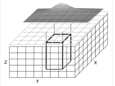
Fig. 2.1: The geosection model (thin line - 3D geosection array, dotted line - 2D surface profiles array, thick line - anomalous body).
The calculation of least squares in the step (4) was reduced in a 2D sub-array window of points over the node in question. The size of the window was correlated with the shape of the element anomaly depending on the element depth in order to consider only the area where the elementary anomaly had significant values greater than the floor 1/K, where K is a predefined number. A sample of normalized anomalies (anomalous values divided by their maximum for each anomaly) for elements in different depths is presented in Fig. 2.2.
During each iteration the density of a single cuboid element of the geosection is updated with a predefined density step. Two alternatives for the iteration termination criteria were investigated:
1. when the decrease in the global least squares error becomes less than a very small predefined value; 2. when the elementary density giving the best approximation within the window results in less than half of the predefined density step.
The calculations for the effect of a single 3D node were considered as an elementary calculation block. The number of elementary calculation blocks for one iteration is equal to Ncalc= (NxNyNz)×(NaNb), where
Fig. 2.2: Normalized elementary anomalies for unitary bodies in different depths 1:10 units; two horizontal lines at the level 0.1 define the least squares windows for floors 1/10 and 1/11.
number of points in linear edges of the 2D rectangular anomaly array. N was considered as a representative of the number of linear nodes / points, and the volume of calculations in one iteration resulted O(N5). The update of the best 3D node in each iteration was done with a fixed density step, and each node was updated until a limit mass density value was obtained. The quotientNdof the mass density limit divided by the density
step is one factor that defines the number of iterations. The overall order of elementary calculations blocks for the whole iterative process would be O(N5N
d), the same stands for the runtime as well. Such high order of
the volume of calculations made the parallelization obligatory in order to obtain inversion results for models of relatively high resolution.
The walltimeTw(difference between the time-stop and time-start of the program) was obtained using the
OpenMP routine omp get wtime(). The linuxtimecommand was used to run the program in order to get the accumulative percentage of CPU usage. The runtime Tr (walltime in case of 100% CPU) was calculated as
Tr=Tw×CP U%/cores .
Basic experiments were carried out for a geosection of 4000m×4000m×2000m digitized with 3D node arrays of step 400m, 200m, 100m and 50m. The anomaly under consideration was calculated in a similar 2D array of points for a vertical prismatic body with density 5 g/cm3 situated at the center of the geosection (Fig. 2.1). More experiments with anomalies calculated for a geosection composed of two vertical prismatic bodies were carried out, as well as with real data from field surveys. Results included inversion geosections with distribution of densities and related anomalies, and the ”carrot” presentation in 3D of distribution of densities in the central vertical section of the geosection for each iteration, showing the progress of the iterative process.
3. Evaluation of Iterative Inversion Process. Two alternatives mentioned before for the termination criteria of the iterative process were compared for arrays with step 200m and 400m, for density steps 0.1g/cm3, 0.5 g/cm3 and 1.0 g/cm3. Both alternatives gave similar number of iterations and of runtime, as shown in Fig. 3.1 for the array with step 200m.
Fig. 3.1: Comparison of number of iterations (left) and runtime in seconds (right) for two termination criteria.
The global relative error achieved by each of termination criteria resulted dependent upon both the array step and the density step, as shown in Fig. 3.2.
span of the anomaly of the surface element (depth 1 unit) was reduced to three nodes (Fig. 2.2) and the iterative process diverged (Fig. 3.3).
Fig. 3.3: Number of iterations, runtime and error for different windows floor factor.
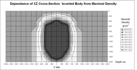
Further tests showed that the algorithm had a tendency to form bodies with the largest mass density. Theoretically, a variation by a factor of k in the mass density of the body would be compensated for by a reversed variation in linear size of the body by a factor ofk(1/3). In our model we used a body with a density of 5g/cm3 and tested the algorithm for maximal accepted densities varying from 1 - 9 g/cm3. The variation in the size of the body at the central vertical 2D section is presented in Fig. 3.4.
Fig. 3.4: Variation of anomalous bodies obtained by inversion for different maximal accepted mass density; the white rectangle represents the original body layout.
Both the theory and the findings supported the idea that keeping a maximal accepted mass density in the range of 2 - 3g/cm3 would be optimal, while higher values would simply lead to a reduction in the size of the body of at most 20%. At the same time the tendency to give larger mass densities is an indication how the algorithm optimizes the solution locally.
Fig. 3.5: Development of the anomalous body central section during inversion iterations (left) and the decrease in the anomaly approximation error (right).
The decrease per iteration in the error of approximation of the anomaly was linear, curving to constant in the final iterations (with a total of 1066 iterations), while delineation of the main section of the body was approximated with half of the iterations.
Fig. 3.6: Two bodies model geosection X-Z (left) and related the anomaly (right).
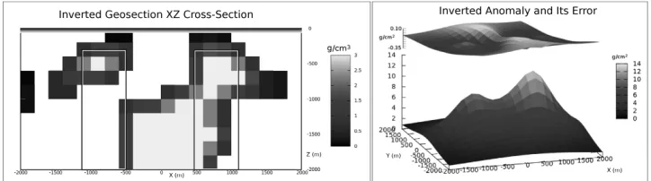
The case of inversion of an anomaly created by a geosection composed of two bodies presented an ill-posed problem. We used a geosection with two vertical prismatic bodies creating a bimodal anomaly (Fig. 3.6). The result of inversion, with a relative least square error of 10%, is shown in Fig. 3.7.
Fig. 3.7: Two bodies inverted geosection X-Z (left) and the related anomaly (right: bottom the anomaly, top: the error).
The error varied between -0.35g/cm2 and +0.1 g/cm2 for the anomaly, which varied between 0.5g/cm2 and 10g/cm2. The inversion gave a three-body geosection, which intuitively may be deduced from the shape of the anomaly itself (apparently a regional anomaly combined with two local anomalies). The progress of delineation of bodies during iterations is given in Fig. 3.8.
Fig. 3.8: Development of the anomalous central section during inversion iterations.
Fig. 3.9: Real case of field anomaly (left bottom), the error (left top) and the inverted geosection (right).
4. Convergence of the Iterative Inversion Process. Parallelization was undertaken using OpenMP, splitting in chunks the 3D array to search in parallel for the best node in each iteration. Parallel calculations were tested in two systems:
1. the HPCG centre at the Institute of Information and Communication Technologies (IICT-BAS) in Sofia, Bulgaria;
2. the NIIFI Supercomputing Centrr at University of P´ecs, Hungary.
Tests in HPCG were done for the anomaly of a vertical prismatic body; with 1, 8 and 16 parallel cores; for geosection arrays with step 400m, 200m and 100m (corresponding to 11, 21 and 41 linear nodes) and density steps 0.1g/cm3, 0.5g/cm3and 1.0g/cm3. Tests were done using the variation of the global error as termination criteria. The number of iterations as a function of the density of the 3D array is presented in Fig. 4.1. Increase in iterations slows down with the increase in the size of the problem. For comparison the line represents the order of O(N4).
The relative least square error as a function of the density of the 3D array is presented in Fig. 4.2. Differently from the iterations, the mass density step had little impact on the error.
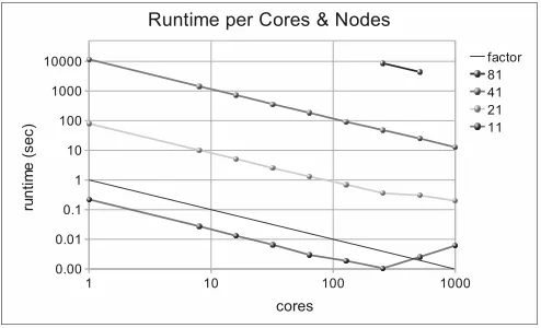
Further tests were done in the NIIFI centre using up to 1024 parallel cores. The number of cores permitted a model to be run with a 3D array step of 50m, which was not possible in HPCG. Given the fact that the resulting error was relatively independent of the mass density step, tests were done only for a density step of 1 g/cm3. The number of iterations and the error for 3D array steps of 400m, 200m, 100m and 50m (respectively 11, 21, 41, and 81 linear nodes) are presented in Fig. 4.3.
The factor line represents the order of O(N3). The results confirmed the slow down in the increase in the number of iterations when the spatial density of geosection nodes is increased. The error apparently does not depend strongly upon the density of the array.
Fig. 4.1: Number of iterations per density of the 3D array; curves represent different mass density steps (the top-down order as in the legend).
Fig. 4.2: Inversion error per density of nodes, curves represent different mass density steps (the top-down order as in the legend).
The maximal processor runtime that was achieved in parallel systems was 3.3 hours in the NIIFI and 21.6 hours in the HPCG.
5. Conclusions. Results of the calculations show that parallel systems may be used successfully for the inversion of geophysical anomalies, but at the same time the process of calculations remains tricky. Even simple algorithms as CLEAN when applied for 3D models required considerable HPC resources (number of cores and cpu runtime), while the results may be disputable in case of complex geosections, and the scalability of the algorithm would decrease when it runs in parallel systems shared by many users.
Utilization of OpenMP resulted in simplification of the programming, but the parallel systems resources available in southeastern Europe were unsuitable for this technology - only one site offered more that 16 parallel cores for OpenMP. Switching towards MPI - based solutions is obligatory and would permit running of software in HPC clusters and grid clusters that are more available than shared memory parallel systems.
Use of simple algorithms in parallel systems was, in terms of runtime and error obtained, successful for geosections with massive bodies; for geosections with thin structures detailed 3D arrays have to be used, which leads to an increase in the runtime to levels that may be difficult to be supported by existing parallel systems available in the region.
In our models the minimal spatial differentiation achieved was 50m using 256 and 512 parallel cores (available only in one site) for a runtime of order of hours. Tests with multiple bodies and real field data reconfirmed the need of using initial solutions defined on the basis of other geological factors, and the need for careful interpretations of results.
Fig. 4.3: Number of iterations and inversion errors per density of 3D array (the top-down order of curves as in the legend).
Fig. 4.4: Scalability of the algorithm and the runtime for number of cores and size of model (the top-down order of curves as in the legend).
REFERENCES
[1] J. Hadamard,Sur les prolemes aux derivees partielles et leur signification physique, Bull Princeton Univ., 13, l-20, 1902. [2] P. Shamsipour, M. Chouteau, D. Marcotte, P. Keating,3D stochastic inversion of borehole and surface gravity data
using Geostatistics, in EGM 2010 International Workshop, Adding new value to Electromagnetic, Gravity and Magnetic Methods for Exploration Capri, Italy, April 11-14, 2010.
[3] F.J. Wellmann, F. G. Horowitz, E. Schill, K. Regenauer-Lieb,Towards incorporating uncertainty of structural data in 3D geological inversion, in Elsevier Tectonophysics TECTO-124902, 2010. http://www.elsevier.com/locate/tecto (re-trieved 07 Sept 2010).
[4] J. A. H¨ogbom,Aperture Synthesis with a Non-Regular Distribution of Interferometer Baselines, in Astr. Astrophys. Suppl., 15, 417, 1974.
[5] P. Rickwood and M. Sambridge,Efficient parallel inversion using the Neighborhood Algorithm, in Geochemistry Geophysics Geosystems Electronic Journal of the Earth Sciences. Volume 7, Number 11, 1 November 2006.
[6] M.H. Loke and P. Wilkinson,Rapid Parallel Computation of Optimized Arrays for Electrical Imaging Surveys, in Near Surface 2009 15th European Meeting of Environmental and Engineering Geophysics Dublin, Ireland, 7-9 September 2009. [7] Hu Zuzhi, He Zhanxiang, WangYongtao, Sun Weibin,Constrained inversion of magnetotelluric data using parallel simu-lated annealing algorithm and its application, in SEG Expanded Abstracts / Volume 29 / EM P4 Modeling and Inversion, SEG Denver 2010 Annual Meeting.
[8] G. Wilson, M. uma, and M. S. Zhdanov,Massively parallel 3D inversion of gravity and gravity gradiometry data, in PREVIEW - The Magazine of the Australian Society of Exploration Geophysicists, June 2011.
[9] W. Lowrie,Fundamentals of Geophysics, Cambridge University Press 2007.