Experimental Analysis of Hybrid Genetic Algorithm for the Grey Pattern Quadratic Assignment Problem

Experimental Analysis of

Hybrid Genetic Algorithm for

the Grey Pattern Quadratic

Assignment Problem

ITC 2/48

Journal of Information Technology and Control

Vol. 48 / No. 2 / 2019 pp. 335-356

DOI 10.5755/j01.itc.48.2.23114

Experimental Analysis of Hybrid Genetic Algorithm for the Grey Pattern Quadratic Assignment Problem

Received 2019/04/08 Accepted after revision 2019/05/09

http://dx.doi.org/10.5755/j01.itc.48.2.23114

Corresponding author: [email protected]

Evelina Stanevičienė

Kaunas University of Technology, Department of Multimedia Engineering, Studentų str. 50-408, LT-51368 Kaunas, Lithuania, tel. +370-37-300373, e-mail: [email protected]

Alfonsas Misevičius

Kaunas University of Technology, Department of Multimedia Engineering, Studentų str. 50-416a/400, LT-51368 Kaunas, Lithuania tel. +370-37-300372, e-mail: [email protected]

Armantas Ostreika

Kaunas University of Technology, Department of Multimedia Engineering, Studentų str. 50-401, LT-51368 Kaunas, Lithuania tel. +370-37-300371, e-mail: [email protected]

In this paper, we present the results of the extensive computational experiments with the hybrid genetic algo-rithm (HGA) for solving the grey pattern quadratic assignment problem (GP-QAP). The experiments are on the basis of the component-based methodology where the important algorithmic ingredients (features) of HGA are chosen and carefully examined. The following components were investigated: initial population, selection of parents, crossover procedures, number of offspring per generation, local improvement, replacement of popula-tion, population restart. The obtained results of the conducted experiments demonstrate how the methodical redesign (reconfiguration) of particular components improves the overall performance of the hybrid genetic algorithm.

KEYWORDS: computational intelligence, heuristics, hybrid genetic algorithms, combinatorial optimization,

Introduction

The grey pattern quadratic assignment problem (GP-QAP) can be considered as a special case of the quadratic assignment problem (QAP) [2]. It is stated as follows [23]. Given two matrices A=( )a_{ij n n}× and

( )b_{kl n n×} =

B and the set ∏_n of permutations of the inte-gers from 1 to n, find a permutation p∈ ∏_n which min-imizes the function z p( ) as described in the following formula:

1 1 ( ) ( )

( ) n n

i j ij p i p j

z p = ∑ ∑= =a b , (1)

where a_ij =1 for i j, =1, ...,m (1≤ <m n)1 _{and 0} ij a = otherwise. In this way, the objective is changed to finding the permutation elements p(1), ..., ( )p m (1≤ p i n i( )≤ , 1, ...,= m) such that the simplified func-tion z p( ) (regarded as an objective function of the GP-QAP) is minimized:

1 1 ( ) ( )

( ) m m

i j p i p j

z p = ∑ ∑= =b . (2)

The values of the matrix B are seen as symmetric distances between each pair of n objects (elements). According to the definition in [23], the distances are calculated by using the following expressions:

2 2

( 1) ( 1)

kl r n s t n u rstu

b =b _{− + − +} =ω _,

1, 2 { 1, 0,1} _{1 1} 2 _{2 2} 2

1 max

( ) ( )

rstu _{w w r t w n r t w n} ω

∈ −

 

 

 

 

 

=

− + + − + ,

(3)

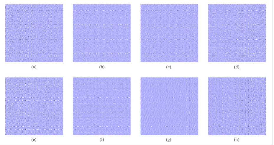
where k l, =1, ...,n, r t, =1, ...,n₁, s u, =1, ...,n₂, n n₁× ₂=n. We have a grid of dimensions n n₁× ₂. More precisely, we have n n n= ×_{1 2} squares in the grid: there are m black squares and n m− white squares. (Other colors may be considered instead of black and white.) This forms a grey (or color) pattern of density m n. And the aim is to have a grey (color) pattern where the black points (color points) are distributed in the most uniform

1  In our work, we will consider m n≤ 2.

possible way2,3_.

For solving the GP-QAP, various optimization tech-niques can be applied, including the exact and heu-ristic algorithms. The exact algorithms are usually only suitable for small-sized problems [4, 6]. For problem instances that cannot be easily solved, heu-ristic algorithms are used. In principle, a huge spec-trum of general-purpose heuristic methods (like single solution-based (trajectory-based) local search algorithms, population-based evolutionary algo-rithms, swarm intelligence algoalgo-rithms, physically and biologically-inspired algorithms) [1] are potentially applicable. To be more precise, a local search-based steepest descent algorithm was examined in [4]. Tabu search methodology-based algorithms were investi-gated in [4, 23, 25]. Evolutionary/genetic algorithms have been shown to be very efficient [4, 23, 24]. The best results were achieved by applying the hybrid al-gorithms, which, in particular, combine the genetic algorithms and tabu search-based procedures [4, 13, 15, 16, 18, 20].

The hybrid genetic algorithms can be seen as ensem-bles of several ingredients, features, i.e., components (like initial population construction, selection of par-ents, crossover procedure, etc.). These components may, in turn, involve alternative options (including

2 The coordinates ( , )r s of the black/color squares are cal-culated according to these formulas: r=_

(

p i( ) 1−

)

n2_+1,

(

)

(

( ) 1 mod 2

)

1

s= p i − n + .

3 The GP-QAP can alternatively also be represented as follows [4]. Let n be the number of points, m be the number of points to be selected out of n points, and dij be the distance between points i and j. Also, let N be the set of n points and let M be the subset (cluster) of selected points. The cardinalities of N and M are equal to n and m, respectively (| |N =n, |M|=m). The subset M can be linked to the permutation elements p(1), ..., ( )p m such that M={p i i( ) : 1, ...,= m} and in similar fashion the set N can be associated with the elements

(1), ..., ( )

p p n where N={p i i( ) : 1, ...,= n}. The goal is to minimize the total distance between all pairs of points in the cluster of m points, that is, the following objective function

( ) _{i M j M ij}

f M = ∑∈ ∑∈ d is to be minimized.

This is similar to the formulation of the maximum diversity problem (MDP) [7, 11], where one wishes to select a subset M of m elements from the set N of n elements in such a way that the sum of pairwise distances between any two elements in M is not minimized but maximized instead.

control parameters). By extracting different partic-ular components and options, we can study their impact and influence [10]. Also, by combining them in a proper way, we can reconfigure the existing algo-rithms; we can find the most promising redesigned al-gorithm architectures and build new powerful «syn-thetic» algorithm variants.

The main contribution of this article is just the demonstration of the benefits of component-based approach and experimental algorithm analysis based on the computational testing of the particular ex-tracted components and options. The novel, original advantageous variants and configurations of combi-nations of algorithmic components and options are introduced and investigated.

The structure of the paper is as follows. In Section 1, a high-level description of HGA for the GP-QAP is giv-en. Section 2 describes the main essential algorithmic components of HGA for the GP-QAP. The results of the computational experiments with the considered algorithmic components are presented in Section 3. The paper is completed with concluding remarks.

1. High-Level Description of Hybrid

Genetic Algorithm for the GP-QAP

Our genetic algorithm is based on the hybrid genetic algorithm framework where the explorative search (i.e., population-based evolutionary search) is in com-bination with the exploitative search (i.e., local im-provement of the produced offspring). (For the pre-cise description of genetic algorithms, the interested reader is advised to refer to the fundamental books on the theory of GAs, e.g., [9, 22].)

Very briefly, our algorithm starts with the creation of an initial population. To ensure the high quality of the initial population, all the population members undergo local improvement (optimization) (see be-low). The genetic algorithm then performs iterations called generations until the pre-defined number of generations, N_gen, has been accomplished. At each generation, the standard genetic operations — selec-tion, crossover, population replacement — take place (without the direct involvement of mutation). Every new solution (offspring) produced by the crossover operator is subject to local improvement. In order to

preserve the diversity of the population members, an enhanced population replacement strategy is ad-opted. On top of this, a population restart (invasion) process is incorporated to renovate the population if the genetic variability is lost and/or idle generations occur. (A more thorough description of this algorithm is presented in [20].)

The structure of our algorithm differs from the tradi-tional usual schemes of genetic algorithms. The fol-lowing are the main differences.

1 No encoding/decoding is necessary. The

permuta-tion elements can be directly associated with in-dividuals’ chromosomes represented as binary bit strings in traditional GAs. (We will use the terms «solutions», «individuals», «chromosomes» in-terchangeably. We will also use the term «gene», where gene in our case corresponds to the single element p i( ) of the permutation p.)

2 The fitness of the individual is associated with the

objective function value corresponding to the giv-en solution. No scaling (recalculation) is needed, except the parent selection procedure (see Sec-tion 2.2.2).

3 The crossover operator is performed at every

gen-eration, i.e., the crossover probability is equal to 1.

4 As a local optimizer, we apply the hierarchical

it-erated tabu search (HITS) algorithm (see Sec-tion 2.5).

5 The mutation process is integrated into the local improvement algorithm (HITS algorithm) as an inherent constituent part of this algorithm.

6 Our algorithm is also distinguished by the fact that

the enhanced population replacement strategy is adopted, so that the attention is paid not only to the quality of the individuals, but also to the genetic di-versity (the mutual difference (distance) between the population members). Only individuals that are diverse enough survive for the next generation.

7 Finally, we utilize the population restart

(«inva-sion») mechanism to withstand the premature convergence and staled evolution. Restart process is triggered in the cases of the apparent stagnation of the genetic process.

2. Components of the Hybrid Genetic

Algorithm for the Grey Pattern

Quadratic Assignment Problem

The following are the essential components of the hy-brid genetic algorithm, which are analysed in this work:

1 INITIAL POPULATION;

2 SELECTION; 3 CROSSOVER;

Note. The parameters InitPopVar, SelectVar, CrossVar, ReplaceVar, RestartVar control the various “scenarios” of the genetic algorithm. The parameter InitPopVar controls the way in which the initial population is created. SelectVar is to choose the particular procedure for parents selection. CrossVar enables to switch between several crossover operators. ReplaceVar and RestartVar are to manage the population replacement and restart processes, respectively.

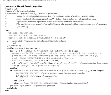
Figure 1

Component-based description of the hybrid genetic algorithmthe hybrid genetic algorithm are discussed in more detail in the subsequent sections. The high-level description of the hybrid genetic algorithm is presented in Figure 1. The particular components of

procedure Hybrid_Genetic_Agorithm_;

// input: n, m, B

// output: p_{− the best found solution}

// parameters: PS − population size, Ngen− number of generations,

// InitPopVar− initial population variant, SelectVar− selection variant, CrossVar− crossover variant, // Noffspr− number of offspring per generation, DT − distance threshold, Lidle_gen− idle generations limit, // ReplaceVar− population replacement variant, RestartVar− population restart variant

// [The local improvement algorithm (hierarchical iterated tabu search algorithm) possesses its own set of parameters // (see Table 2)]

begin

get data, parameters;

initialize algorithm variables;

create (sorted) INITIAL POPULATION P _{of size} PS_;

: arg min{ ( )} p P p∗ z p

∈

= _// memorize the best solution of the initial population

gen_index_:= 1;

while gen_index≤ Ngen do begin

for i:= 1 to NUMBER OF OFFSPRING PER GENERATION do begin

perform SELECTION procedure to choose the parents p′, p′′∈P for reproduction;

produce one (or two) offspring by applying CROSSOVER operator to p′, p′′_;

apply LOCAL IMPROVEMENT to the produced offspring,

get an (improved) solution p (and p );

if z(p ) <z(p) (or _z(_p ) <_z(_p)) then _p:=_p (or _p:=_p )_; // memorize the best found solution

add p (and p ) to a pool of offspring

endfor;

if number of idle generations exceeds the pre-defined limit Lidle_gen then begin

POPULATION RESTART; // perform population restart (re-construction) procedure

if min{ ( )} ( )

p Pz p z p

∗

∈ < then p : arg min{ ( )}_{p P} z p ∗

∈

=

end // of if

else perform POPULATION REPLACEMENT; // update (and sort) the population P

gen_index:=gen_index+ 1 // go to the next generation

endwhile

end.

Note. The parameters InitPopVar, SelectVar, CrossVar, ReplaceVar, RestartVar control the various "scenarios" of the genetic algorithm. The parameter InitPopVar controls the way in which the initial population is created. SelectVar is to choose the particular procedure for parents selection. CrossVar enables to switch between several crossover operators. ReplaceVar and RestartVar are to manage the population replacement and restart processes, respectively.

Figure 1. Component-based description of the hybrid genetic algorithm

2. Components of the Hybrid Genetic Algorithm for the Grey Pattern Quadratic Assignment Problem

The following are the essential components of the hybrid genetic algorithm, which are analysed in this work: 1. INITIAL POPULATION;

2. SELECTION; 3. CROSSOVER;

4. NUMBER OF OFFSPRING PER GENERATION; 5. LOCAL IMPROVEMENT;

6. POPULATION REPLACEMENT; 7. POPULATION RESTART. 2.1. Initial Population

The initial population component is the component that determines the way in which the initial (starting) population of solutions (individuals) is constructed. There are several options for this component (in other words, there are several variants of the creation of initial population) [17]. For this component, we will use a short syntactic notation in the form of IPx, where IP is the abbreviation for INITIAL POPULATION and x denotes the number of the option. Similar syntax will be used also for other components.

4 NUMBER OF OFFSPRING PER GENERATION;

5 LOCAL IMPROVEMENT;

6 POPULATION REPLACEMENT; 7 POPULATION RESTART.

2.1. Initial Population

oth-er words, thoth-ere are sevoth-eral variants of the creation of initial population) [17]. For this component, we will use a short syntactic notation in the form of IPx, where IP is the abbreviation for INITIAL POPULA-TION and x denotes the number of the option. Similar syntax will be used also for other components. 2.1.1. Randomly Generated Population

In the simplest way, the genetic algorithm starts from a pure random population. No additional actions (i.e., improvement of the members of initial population) are involved. We denote this option as IP1.

2.1.2. Improved Population

In the remaining options, the improvement of the in-dividuals of initial population is involved. In fact, the initial population is constructed in two steps: 1) ran-dom generation, 2) improvement of the generated in-dividuals. In the second step, all the members of the population are subject to improvement by a given lo-cal improvement algorithm (see Section 2.5).

There are the following available options for the im-proved initial population: uniformly imim-proved pop-ulation (IP2), uniformly extra improved population (IP3) and non-uniformly improved population (IP4). A  Uniformly Improved Population

Any local search methodology-based algorithm can be used for the improvement of initial population, for example, tabu search (which is just the case of the present paper). As long as the time spent for the im-provement is essentially the same for each population member, the resultant population may be thought of as uniform (with respect to the fitness of the individ-uals).

Let ℑ be the (default) number of iterations of the lo-cal optimizer. Then, the overall number of iterations used for the construction of initial population is equal to PS_C1⋅ℑ_C2, where PS_C1 =C PS₁⋅ , ℑ_C2 =C₂⋅ℑ. Here, PS denotes the (default) population size and C₁,

2

C are user-defined parameters (weights) such that 1 1

C ≥ , C₂ ≥1. The parameter C₁ regulates the size of the pre-initial population, so that, after improvement of the pre-initial population, (C₁− ⋅1) PS worst mem-bers of this population are truncated and only PS best members survive. This strategy slightly resembles a compounded approach proposed in [3], where several starting populations are maintained and the individ-uals of every population are improved.

The parameter C₂ determines the actual total number of iterations used by the local optimizer during the construction of pinitial population, so that the re-sulting number of improvement iterations during the initialization phase is equal to C₂⋅ℑ.

If C₁=1 and C₂=1, we get the option IP2, otherwise (C₁>1 and/or C₂>1) the option IP3 is obtained. Ob-viously, the larger the values of C₁, C₂, the larger is the probability that the quality of the initial population will be better. However, note that if time-consuming local optimizer is applied, then the overall number of GA’s generations should be accordingly decreased to keep the run time fixed.

B Non-Uniformly Improved Population

In this particular case, the number of improvement iterations at the population initialization stage is not constant, but varies according to some rule, so that the law of distribution of the fitness of individuals of the obtained population is rather non-uniform (for example, normal-like or Gaussian-like). This concept is linked to what is known as «differential improve-ment» approach [5], where more intensive improve-ment is performed on some selected solutions. In our algorithm, the initial population con-struction procedure can be chosen from three variants: IP1, IP2 and IP3. To operation-alize this, a choice-text parameter named

{" ", " ", " "} InitPopVar∈ _{rand_p unif_p extr_p} is used to decide which of these variants will be acti-vated. If InitPopVar="_{rand_p}", IP1will be is used; if InitPopVar="_{unif_p}", IP2 is activated, other-wise IP3 will be operational. In the cases of the op-tions IP2, IP3, our algorithm keeps checks on all improved solutions. That is, after improvement of the particular solution, it is checked if the distance be-tween the improved solution p _{and the population} P ( ( , ) min{ ( , )}

p P

p P p p

δ δ

∈

=

  4_{) is greater than or equal}

to the pre-defined distance threshold, DT. If it is the case, the improved solution is included into the pop-ulation (the same is true if the improved solution is better than the best population member). Otherwise, the randomly generated solution enters the popula-tion. This is to ensure the genetic variance of the ini-tial population. (More details on the construction of initial population can be found in [20].)

4 The distance δ between two solutions p1 and p2 is calculated according to this formula:

1 2 1 2

( , )p p m { ( ) : 1, ..., } { ( ) : 1, ..., }p i i m p i i m

2.2. Selection

This component is used to decide how the parental solutions (chromosomes) for reproduction are cho-sen. The following are the popular selection rules: random selection (S1), roulette wheel (fitness propor-tionate) selection (S2) and rank-based selection (S3). 2.2.1. Random Selection

The elementary option is to choose the parental chro-mosomes in a pure blind random way (the fitness of the parents is not taken into account).

2.2.2. Roulette Wheel Selection

The roulette wheel selection is a fitness-based selec-tion mechanism where the fitness of parents is pro-portional to the value of the objective function calcu-lated for the recalcu-lated solutions.

In the case of roulette wheel selection [9], the scaled fitness values are utilized instead of the raw values of the objective function. The rule of selection is based on the roulette wheel criterion, which assigns to indi-vidual i in the population of PS individuals a selection probability Pr_i proportional to the fitness value of the individual as in this equation:

1 i i _PS j j F Pr F = =

∑ , where Fi,

j

F are scaled fitness values5_. 2.2.3. Rank-Based Selection

Assume that all the members of the current popula-tion are sorted in the ascending order of their fitness (or the objective function values). Then, according to the rank-based rule [26], the positions (u and v) of the parents within the sorted population P are deter-mined by the formulas: u _( )_ξ1 σ_

=  , v= ( )ξ2 σ_, u v≠ ; here ξ₁, ξ₂ are distinct uniform random numbers from the interval _1,PS1σ_

 , where PS is the population size, and σ _{is a real number in the interval}

_{[ ]}

_{1, 2 (}σ _is

5  The scaled fitness Fi can be calculated as follows: F k f ki= 1i+ 2,

where 1 ₍ (1 f) ₍₁avg _{) )}

min f max f avg

S f k

f S f S f

− ×

=

× − + − × , k2= −(1 k1)×favg, Sf is the scaling factor, favg, fmin, fmax are respectively the average,

min-imum and maxmin-imum fitness values before scaling. f_i is a raw fit-ness value (fitfit-ness before scaling) of the ith individual, which is linked to the objective function value through the following rela-tion: 0, ( )

1 ( ) , otherwisei

i i

z p zerofit f

z p zerofit > 

=  ₋

 , here z p( )i is the objective function value corresponding to the ith individual, zerofit K W= × , K is a coefficient, W is the lower bound or the best known value of the objective function for a given problem instance (for more details, see [12]).

referred to as a selection factor). It is obvious that the better the individual, the larger probability of select-ing it for the crossover.

The choice-text parameter SelectVar∈{"_{rand_sel rw_sel rb_sel}", " ", " "} {" ", " ", " "}

SelectVar∈ _{rand_sel rw_sel rb_sel} is utilized to choose between three options: S1 (SelectVar="rand_sel"), S2 (SelectVar="_{rw_sel}") and S3 (SelectVar="_{rb_sel}"). 2.3. Crossover

Crossover operators play a very important role in ge-netic algorithms. One of the main purposes of cross-over is to diversify the search process by recombining the genetic information present in the parental chro-mosomes. It is highly desirable that the crossover process be explorative enough to be capable of discov-ering new regions in the search space (space of poten-tial solutions).

There is a great variety of the crossover procedures, which are usually oriented to work on binary bit strings [21]. However, in the GP-QAP, the chro-mosomal locations of genes are irrelevant, so the straightforward replication of standard procedures to the GP-QAP might not be effective. Anyway, it is important to preserve shared elements of predeces-sors during the recombination process. Based on the shared elements, a concept of backbone solutions is defined. The solution p∈ Π_{n is a backbone} tion (with respect to two underlying parental solu-tions p₁, p₂) if the inequalities δ(p, )p₁ ≤ _m 2__,

2

(p , )p m 2

δ  ≤ _ _{ simultaneously hold; here δ} de-notes the distance between solutions. The back-bone solution thus shares information with its both underlying solutions and is close enough to both of them (or possibly equivalent to them in the sense that

1

(p , ) 0p

δ  = _and/or

2

(p ,p ) 0

δ  = _).

Foreign genes (the genes that are not present in the parents) may also be useful. Such genes may be thought of as opposite genes — opposition-based genes. The solution p∈ ∏n is an opposition-based solution with respect to the given solution p if

δ( )

ä p, p = m. The opposition-based solutions might possibly be more preferable than purely randomly generated solutions [28].

new genes. The crossover operators that follow these conceptions (conceptions of backbone and opposi-tion-based solutions) are known as a backbone-based crossover (C1) and backbone and opposition-based crossover (C2). Similar to them are the multi-parent backbone-based crossover (C3) and multi-parent back-bone and opposition based crossover (C4).

The other promising conception is to adopt the greedy-based approach by choosing the genes from the parents. This principle is put into practice in the greedy crossover (C5) and greedy opposition-based crossover (C6).

There are also crossover procedures which take into account the problem-specific information and are tailored to the particular properties of the problem. An example is the averaging crossover (C7), which is based on calculating the average integer value be-tween the two corresponding values in the parental solutions. A specific crossover operator entitled as tabu merging process (C8), which is proposed in [4], also belongs to this type of crossover procedures. Finally, an extra variant is possible with no crossover at all (C9). This option may be viewed as an asexual self-replication.

The parameter CrossVar∈{" ", " ", " ", " ", " ", " ", " ", " ", " "}1 2 3 4 5 6 7 8 9

{" ", " ", " ", " ", " ", " ", " ", " ", " "}

CrossVar∈ 1 2 3 4 5 6 7 8 9 serves as a switch between nine options: C1, …, C9. All the crossover operators corre-sponding to these options (including the crossover from [4]) are implemented by the authors of this pa-per6_{. Some operational implementation aspects are as} follows.

To create the backbone solution, it is enough to main-tain one-dimensional array of gene frequency values,

freq. The values of freqare calculated by this expression:

{

}

( ) : { ( ) : 1, ..., }, { ( ) : 1, ..., } freq i = i i∈ p' j j= m i∈ p'' j j= m , where i=1, ...,n and p', p'' are the parental solutions (more than two parents may be used). The m genes with the largest frequency values are then picked up (ties are broken randomly). The chosen genes consti-tute the backbone solution.

The obtained solution can be partially optimized to ensure a higher quality of the offspring. A greedy adap-tive procedure (GAP) is applied for this purpose. The GAP receives a partial (backbone) solution _p~ _(the

el-6 The source texts (in C# programming language) of the crossover operators can be found at: https://www.personalas.ktu. lt/~alfmise/

ements _p~_{(1), ..., p}~_{( )γ ) as an input. The integer} num-ber γ (0< <γ m) is the controlling parameter for the GAP, which determines the actual size of the partial solution. The GAP chooses the element, one at a time, and adds it to the current partial solution. In partic-ular, GAP adds at each iteration q (q=1, ...,m−γ) the element from the set of unselected elements with the minimum possible contribution to the value of the ob-jective function. This is continued until the solution is completed. The detailed description of GAP is pro-vided in [20].

In the case of greedy crossover, the same procedure is used, except that γ =0 (which means that the input solution is empty) and that the elements are chosen from the parental solutions.

Regarding the opposition-based solution, this is op-erationalized by maintaining a long-term memory ar-ray ltm, where ltm i( ) contains the number of times the element (gene) i ever appeared in an offspring solu-tion. The memory is initialized with zeros once before starting the genetic algorithm. Its values are updated whenever a new offspring solution is created. To ob-tain the opposition-based solution, it is sufficient to pick up m items with the smallest frequency from the long-term memory (ties are broken randomly). 2.4. Number of Offspring per Generation

This is to control how many offspring are created be-fore updating the current population and continuing with the next generation. Usually, in the standard ver-sions of GAs, a single offspring per generation is pro-duced. We call this option single offspring (NOG1). The other options are also possible, where several off-spring are created [19]. For example, suppose that λ offspring are produced (in our algorithm, λ=N_offspr). In other words, a generation consists of producing λ offspring. With this, we are a bit closer to the nature. We can assign a «juvenile» status for all newly born offspring, so that the juveniles are not reproductive for some time. By the next generation, the juveniles develop into adults and become reproductive.

gen-eration, PS individuals are selected out of PS+λ indi-viduals to form the new population for the next gener-ation (also see Section 2.6).

Note that if the number of offspring is increased (λ >1), then the total number of generations should be ac-cordingly decreased in order to stay within the same run time.

2.5. Local Improvement

The local improvement (local optimizer) is very likely the most important component of the hybrid genetic algorithm. In contrast to the crossover operator, this component is responsible for the intensification of the search process. It is rather exploitative and con-centrates the search in rather limited areas of the search space, staying in the neighbourhood of the off-spring solution. Various heuristic algorithms can be adopted for this task. In most cases, these are the sin-gle solution-based algorithms, which get the offspring solution as an initial solution and return (a possibly) improved solution for the further consideration. In this work, we use the hierarchical iterated tabu search approach, where the basic principle is to mul-tiply reuse the tabu search (TS) [8] algorithm. We remind that the main idea of tabu search is based on the prohibition of returning to the solutions that have been visited recently. The prohibition period, i.e., the tabu tenure is one of the controlling parameters of TS. The memory structure called a tabu list is used for the prohibited solutions. In our case, the TS process itself consists of iterations trying to interchange the elements of the current solution. In particular, TS it-eratively swaps an element of the set { ( ) :p i i=1, ..., }m with another element of the set { ( ) :p j j m= +1, ..., }n . If the found best solution is not in the tabu list or the tabu aspiration criterion is satisfied, then the new ob-tained solution replaces the current one. A secondary memory is utilized to archive high-quality solutions. The TS procedure restarts from time to time from one of these solutions if the minimum objective function value is not improved for L_{idle iter_} iterations. Addition-ally, we apply a special technique [27] to reduce the number of interchangeable elements during the TS procedure (for more details, see [20]).

The HITS algorithm is kth-level7 _{iterated tabu search} (ITS) algorithm, which consists of ( 1)k− th-level ITS

7 We used k=7.

algorithm, candidate acceptance rule and perturba-tion procedure. The kth-level ITS algorithm trans-forms the current solution into the optimized solu-tion using ( 1)k− th-level procedure. Perturbation is applied to the chosen optimized candidate solution, which is selected by a defined candidate acceptance rule. The perturbed solution serves as an input for the ( 1)k− th-level procedure, which starts immediately after the perturbation process has been executed. The ( 1)k− th-level algorithm includes the (k−2)th-level algorithm, and so on (all the way down to the 0th-level procedure). The best found solution is the result of the HITS algorithm.

The solution perturbation procedure consists of ran-dom mutation (shuffling) and reconstruction of the mutated solution. For reconstruction, we use the greedy adaptive procedure (see Section  2.3), where

mut

m

γ = −µ , here µmut is referred to as a mutation rate. (More details can be found in [20].)

Assume that the (default) total number of (global) iterations of the hierarchical iterated tabu search al-gorithm is equal to ℑ; meanwhile, τ is the number of (internal) iterations of the self-contained tabu search procedure (in our algorithm, ℑ =Q_hier). The pertur-bation procedure (including the mutation process) is then performed once every τ iterations. We will call this scheme (( , ,1)ℑ τ -scheme) as a neutral variant (LI1). The other options (schemes) are as follows. 2.5.1. Diversified Quick Search

If the value of τ _{is decreased and the value of} ℑ re-mains constant, this means that the search process is rather quick and, at the same time, diversified, scat-tered over several regions in the search space. We call this option diversified quick search (LI2). (In particu-lar, we use the scheme ( , 2,1)ℑ τ in our experiments.) 2.5.2. Extensive Search

On the contrary, if the value of τ is increased (and the value of ℑ stays unchanged), this means that the search process is quite intensive, rather extensified than diversified. We refer to this option as exten-sive search (LI3). (Particularly, we use the scheme ( , 2 ,1)ℑ τ in our work.)

2.5.3. Quick Search

which is pretty quick (like in the option LI2), but is not so diversified (scattered). We call this option quick (localized) search (LI4). (The scheme ( 2 , ,1)ℑ τ is, in particular, used in this work.)

2.5.4. Diversified Extensive Search

Finally, if the value of τ stays constant and the val-ue of ℑ is increased, this leads to the search process which is relatively extensive (like in the option LI3); at the same time, the search is diversified, rather than concentrated in some localized region. This option is termed as diversified extensive search (LI5). (The scheme (2 , ,1)ℑ τ is, particularly, used in our experi-mentation.)

The number of generations of HGA should be accord-ingly adjusted in the case of options LI2−LI5 (in or-der to stay within the fixed run time).

2.6. Population Replacement

The purpose of this component is to update the pop-ulation according to some pre-defined strategy. Two basic population replacement policies are steady state replacement and generational replacement [22]. In the first case, new individuals are inserted into the cur-rent population as soon as they are produced. In the generational replacement strategy, an intermediate population (pool) is usually created before updating the current population. This means that individuals can only reproduce with individuals from the same generation before moving to the next generation. Two popular generational replacement strategies are known as the "µ λ+ "-update and " , "µ λ -update. Suppose that the size of a population is equal to µ and the number of newly created individuals is equal to λ (in our algorithm, µ=PS, λ=N_offspr). Then, in the case of "µ λ+ "-update, the individuals chosen for the next generation are the best µ members of Pµ∪Pλ, where Pµ is the current generation’s population and

Pλ denotes the pool of newly created individuals. (For example, if λ =1, then the single offspring simply re-places the worst member of the population (provided that the offspring is better than the worst population member — otherwise, the offspring is ignored).) In the " , "µ λ scheme, λ new individuals replace their related predecessors in the current population. Typ-ically, the children replace their worse parents. The fitness of the children is not taken into consideration.

Based on these standard strategies, modified strate-gies may be introduced. In the schemes we formally denote as "µ λ ε+ , "-update and " , , "µ λ ε -update, a minimum distance criterion is introduced. That is, after the offspring solution is improved, it is checked whether the new solution (p_{) differs enough from} the other solutions in the population. Particularly, it is checked if the minimum distance between the new solution and the remaining members of popula-tion (  ( , ) min{ ( , )}

p P

p P p p

δ δ

∈

=

  _{) is not less than the}

distance threshold, ε (in our algorithm, ε =DT (see Section 2.1.2)). If this condition is not satisfied, the new solution is not allowed to enter the population (unless the new solution is better than the best pop-ulation member). These modified strategies are to maintain the sufficient diversity of the members of population.

Based on the above strategies, the following replace-ment options are considered: worst individual con-ditional replacement (or PR1according to our rule of notation), worst individual unconditional replacement (PR2), modified conditional replacement (worst-or-best update) (PR3), worse parent conditional replace-ment (PR4), worse parent unconditional replacement (PR5). (Let the value of λ be equal to 1 without a loss of generality.)

2.6.1. Worst Individual Conditional Replacement In this particular case, the newly produced offspring solution simply takes the place of the worst member of the current population, but under the necessary condition that the new offspring is better than the worst individual in terms of the objective function value. The minimum distance criterion must be sat-isfied, i.e., the condition min{ ( , )}

p P∈ δ p p ≥ε

 _{must hold}

for the offspring solution p_{. If this criterion is not}

met, the offspring is deleted (the population remains unaltered) and the algorithm continues with the next generation. (Note, however, that this criterion is disobeyed if the offspring appears better than the best population individual.)

2.6.2. Worst Individual Unconditional Replacement

2.6.3. Modified Conditional Replacement

This is similar to the option PR1. Additionally, it is tested if the offspring is better than the best individ-ual of the current population. If this is the case, then exactly the best individual (rather than the worst in-dividual) is replaced. Again, the minimum distance criterion must be fulfilled.

2.6.4. Worse Parent Conditional Replacement The current option is also very close to the option

PR1. The only difference is that the offspring replac-es its rreplac-espective worse parent (but not the worst in-dividual) if only the offspring is better than its relat-ed parent with respect to the value of the objective function.

2.6.5. Worse Parent Unconditional Replacement This option is very similar to the option PR4, except that the successor solution automatically replaces its respective worse predecessor disregarding the fitness of the predecessor.

It should be noted that in all above options, the sur-vival of the best member in the population is ensured. This aspect is commonly known as elitism.

The parameter ReplaceVar∈{"_{wi_r_1 wi_r_2 mod_r wp_r_1 wp_r_2}", " ", " ", " ", " "} {" ", " ", " ", " ", " "}

ReplaceVar∈ _{wi_r_1 wi_r_2 mod_r wp_r_1 wp_r_2} is utilized to oper-ationalize the replacement process. The following is the correspondence between the parameter values and the actual replacement options: "wi_r_1" — PR1, "_{wi_r_2}" — PR2, "_{mod_r}" — PR3, "_{wp_r_1}" — PR4, "wp_r_2" — PR5.

2.7. Population Restart

The population restart (invasion) component also plays an important role since it is responsible for diversification of the evolutionary search in the sit-uations where the diversity of the individuals is lost and the search process becomes stagnated [14]. In such cases, some mechanisms should be incorporat-ed to restart the overall process by starting from the renovated (regenerated) population. These mecha-nisms differ in essence in how the new population is obtained. Two main opposite strategies may be seen as «hot restart» and «cold restart». In the hot restart, only small perturbations are applied to the stagnated population, whereas large population changes take place in the case of the cold restart.

The rate (frequency) at which the restarts occur is also a very significant factor by designing the re-start-based genetic algorithm.

The simplest option is no restarts (PRS1). In this case, no restarts are involved at all.

2.7.1. Restart from Random Population

This option is to disregard all the individuals of the current population and generate new random popula-tion from scratch. This may be seen as a restart from new random population (PRS2).

2.7.2. Multi-Mutation

The restart from an entirely new population may seem too aggressive. A more gentle option is multi-mutation, where mutation process is applied to all the members of population instead of complete-ly destroying the current population. The advantage of mutation is that the strength of mutation can be flexibly controlled by the user. For example, the user can decide to choose between strong multi-muta-tion (PRS3) (50% of genes are mutated) and mild multi-mutation (PRS4) (10% of genes are mutated). 2.7.3. Opposition-Based Reconstruction

The next option is called opposition-based reconstruc-tion (PRS5). In this particular case, the newly built solutions are not purely randomly generated solu-tions. Instead, they are opposition-based (opposite) solutions with respect to the existing solutions of the stagnated population. The rule of construction of op-posite solutions is analogous to that used in the oppo-sition-based crossover operators.

2.7.4. Gene Translocation

Gene translocation (PRS6) procedure is slightly sim-ilar to the multi-parent crossover procedure. The distinguishing feature is that many children are pro-duced instead of a single child. The principle is: «ma-ny-parents-many-children». The genes «migrate» be-tween the chromosomes of all the individuals in the population. Usually, «foreign» genes are excluded and there are no explicit mutations, which are the case of multi-mutation.

2.7.5. Chaotic Generation

means of chaotic logistic mapping function (logistic map)8_:

1 (1 )

l l l

x+ =rx −x , where xl is a real number be-tween zero and one (in our case, x₀=0.49), l=0,1, ...;

r is a parameter (in our case, r=4.0). This way, the real numbers x x₀, , ...₁ are used to constitute the ran-dom sequences of genes of the new population. This option is denoted as PRS7.

In our algorithm, the restart process is triggered if the solutions of the population are not improved for

_

idle gen

L generations (here L_{idle gen_} is an idle genera-tions limit). After restart, all renovated individuals are improved by the local optimizer using the in-creased number of iterations, Q_rhier (see Table 2). The parameter

{

" ", " ", " ", " ",

}

" ", " ", " "

RestartVar∈ _{oppos gene_trans chaot_gen}no_rest rest_rand_p strong_mut mild_mut

{

" ", " ", " ", " ",

}

" ", " ", " "

RestartVar∈ _{oppos gene_trans chaot_gen}no_rest rest_rand_p strong_mut mild_mut

serves as a switch between seven options: PRS1, …,

PRS7. The correspondence between the param-eters and options is as follows: "_{no_rest}" —

PRS1, "rest_rand_p" — PRS2, "strong_mut" — PRS3, "_{mild_mut}" — PRS4, "oppos" — PRS5,

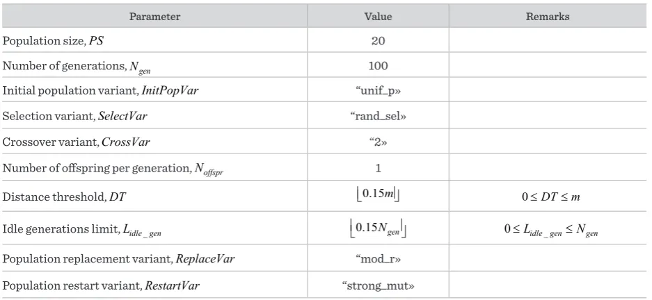
Table 1

Values of the control parameters of the basic configuration of hybrid genetic algorithm

Parameter Value Remarks

Population size, PS 20

Number of generations, N_gen 100

Initial population variant, InitPopVar “unif_p»

Selection variant, SelectVar “rand_sel»

Crossover variant, CrossVar “2»

Number of offspring per generation, Noffspr 1

Distance threshold, DT _0.15m_{ 0≤DT m≤}

Idle generations limit, Lidle gen_ _0.15Ngen_ 0≤Lidle gen_ ≤Ngen

Population replacement variant, ReplaceVar “mod_r» Population restart variant, RestartVar “strong_mut»

"gene_trans" — PRS6, "chaot_gen" — PRS7. All the restart procedures are implemented by the au-thors of this paper.

Before presenting the results of the computational experiments, we declare the following collection (set) of options — IP3, S1, C2, NOG2, LI1, PR3, PRS2 — as the «basic configuration» of our hybrid genetic algo-rithm. The choice of these particular options is on the basis of the preliminary experimentation described in [20] and also the pre-experimental knowledge and experience. The values of the control parameters corresponding to the basic configuration (variant) of HGA are presented in Tables 1 and 2. The basic con-figuration is shortly denoted by BASIC.

For the modified configurations of HGA, we will use short notations like IP1, S3, and so on. For example, the notation IP1 means that the assemblage of options

of the corresponding configuration of HGA is ob-tained from the basic set of options by simply remov-ing the existremov-ing option (IP3) and replacing it by the new option (IP1) (IP1 ≡ IP3, S1, C2, NOG2, LI1, PR3,

PRS2 \ IP3 ∪ IP1.

8

3. Computational Experiments

Our hybrid genetic algorithm was implemented by us-ing C# programmus-ing language. The C# 5.0 compiler was used with the flag «Optimize code». The compu-tational experiments have been carried out on a per-sonal computer running Windows 7 Enterprise. The CPU parameters are as follows: model − Intel Core i5-3450, cores − 4, instruction set − 64 bit, base frequen-cy − 3100 MHz.

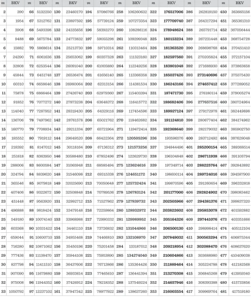
We have tested our algorithm on the medium and large-scaled GP-QAP instances with n=256 and

1024

n= , respectively. These instances are generated according to the method described in [23]9_{. The grids} are of dimensions 16 16× (n₁=n₂ = 16) and 32 32× (n n₁= ₂ =32), respectively. The values of the grey den-sity parameter m varies from 95 to 104 for n=256. For

1024

n= , the values of m are as follows: 50, 60, 70, 80, 90, 100, 110, 120, 130, 140.

As a performance criterion for our algorithm, we use the average relative percentage deviation (θ) of the yielded solutions from the best known

solu-9 These instances can also be found at the website: https://www. personalas.ktu.lt/~alfmise/.

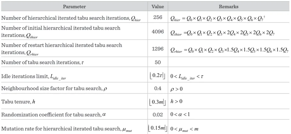
Table 2

Values of the control parameters of the local improvement algorithm (hierarchical iterated tabu search algorithm)

Parameter Value Remarks

Number of hierarchical iterated tabu search iterations, Q_hier 256 Q_hier=Q Q Q Q Q Q Q Q₀× ×_{1 2}× ₃× ₄× ₅× ₆× ₇†

Number of initial hierarchical iterated tabu search

iterations, Qihier 4096 Qihier =Q Q Q Q0× ×1 2× 3×2Q4×2Q5×2Q6×2Q7 Number of restart hierarchical iterated tabu search

iterations, Q_rhier 1296 Qrhier=Q Q Q Q0× ×1 2× 3×1.5Q4×1.5Q5×1.5Q6×1.5Q7

Number of tabu search iterations, τ 50

Idle iterations limit, Lidle iter_ 0.2τ 0<Lidle iter_ <τ Neighbourhood size factor for tabu search, ρ 0.4 ρ>0

Tabu tenure, h _0.3m_ h>0

Randomization coefficient for tabu search, α 0.02 0< <α 1

Mutation rate for hierarchical iterated tabu search, µ_mut _0.15m_{ 0}<µ_mut<_m

† 

0 1 2 3 4 5 6 7 2

Q =Q Q= =Q Q= =Q Q= =Q = . Q0, ...,Q7 denote respectively the corresponding numbers of iterations of the 0th-level, …,

7th-level iterated tabu search algorithm.

tion (BKS). It is calculated by the following formula:

[ ]

100(z BKV BKV) %

θ = − , where z is the average

objective function value over 10 runs of the algorithm, while BKV denotes the best known value of the objec-tive function that corresponds to the BKS. (BKVs are from [20].) At every run, the algorithm is applied to the given values of n and m, each time starting from a new random initial population. Note that the current run is interrupted if BKS is found, even without reaching the maximum number of generations, N_gen.

Firstly, we have experimented with the following con-figurations (variants) of HGA:

1) BASIC, 2) IP1, 3) IP3, 4) S2, 5) S3, 6) C1, 7) C3, 8) C4, 9) C5, 10) C6;

11) C7, 12) C8, 13) C9, 14) NOG1, 15) NOG3, 16) NOG4, 17) LI2, 18) LI3, 19) LI4, 20) LI5;

21) PR1, 22) PR2, 23) PR4, 24) PR5, 25) PRS1, 26) PRS3, 27) PRS4, 28) PRS5, 29) PRS6, 30) PRS7.

Some configurations are omitted for the sake of brev-ity, because we think that the results of these configu-rations are of insufficient quality.

Table 3

Results of the comparison of different configurations (variants) of HGA (n = 256)(part I)

m BKV‡ θ

‡‡

Time‡‡‡

(sec.)

BASIC IP1 IP3♣ _{S2 S3 C1 C3 C4 C5 C6}

95 48081112 0.021 0.077 0.000 0.020 0.014 0.011 0.015 0.021 0.005 0.017 80

96 49182368 0.057 0.134 0.014 0.078 0.080 0.078 0.077 0.080 0.074 0.085 120

97 50344050 0.053 0.105 0.000 0.033 0.062 0.048 0.039 0.061 0.046 0.031 100

98 51486642 0.079 0.120 0.023 0.104 0.083 0.095 0.082 0.083 0.086 0.086 120

99 52660116 0.085 0.105 0.023 0.079 0.074 0.074 0.069 0.077 0.071 0.078 120

100 53838088 0.076 0.082 0.040 0.075 0.069 0.069 0.054 0.075 0.056 0.077 130

101 55014262 0.085 0.096 0.042 0.078 0.083 0.079 0.075 0.077 0.076 0.086 120

102 56202826 0.081 0.092 0.050 0.088 0.082 0.088 0.071 0.081 0.071 0.078 110

103 57417112 0.047 0.070 0.026 0.052 0.054 0.052 0.052 0.055 0.051 0.067 110

104 58625240 0.026 0.073 0.017 0.031 0.040 0.021 0.026 0.041 0.028 0.034 110

Average: 0.061 0.095 0.024 0.064 0.064 0.062 0.056 0.065 0.056 0.064

‡ _{BKV − the best known value;}

‡‡ _{θ − average relative percentage deviation from the best known value;} ‡‡‡ _{average CPU time per one run;}

♣ _{enlarged number of iterations of the hierarchical iterated tabu search for the initial population improvement is used (}

2 4

C = ).

Notes. 1. In the case of S2, we used S_f =3, K=5 (see Section 2.2.2). 2. In the case of S3, we used σ =2.0 (see Section 2.2.3). 3. In the cases of

C1, C2, we used γ= _m2_ (see Section 2.3). In all cases, enlarged pre-initial population is used (C₁=2).

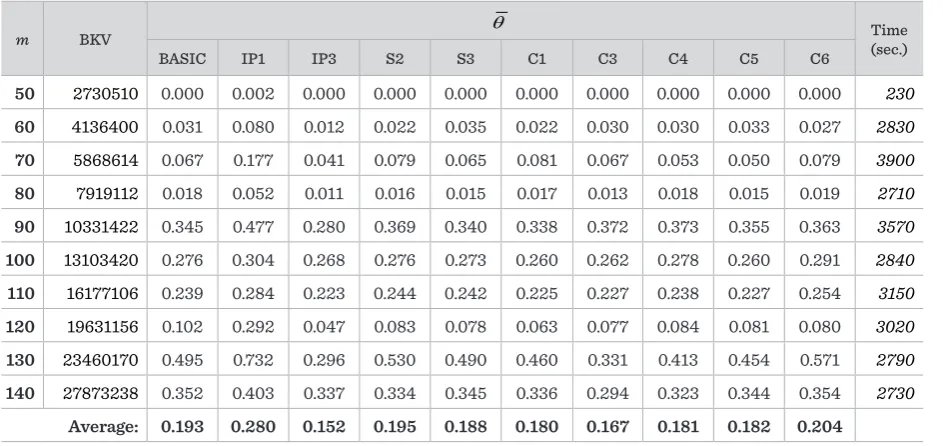
Table 4

Results of the comparison of different configurations (variants) of HGA (n = 1024) (part I)

m BKV θ _(sec.)Time

BASIC IP1 IP3 S2 S3 C1 C3 C4 C5 C6

50 2730510 0.000 0.002 0.000 0.000 0.000 0.000 0.000 0.000 0.000 0.000 230

60 4136400 0.031 0.080 0.012 0.022 0.035 0.022 0.030 0.030 0.033 0.027 2830

70 5868614 0.067 0.177 0.041 0.079 0.065 0.081 0.067 0.053 0.050 0.079 3900

80 7919112 0.018 0.052 0.011 0.016 0.015 0.017 0.013 0.018 0.015 0.019 2710

90 10331422 0.345 0.477 0.280 0.369 0.340 0.338 0.372 0.373 0.355 0.363 3570

100 13103420 0.276 0.304 0.268 0.276 0.273 0.260 0.262 0.278 0.260 0.291 2840

110 16177106 0.239 0.284 0.223 0.244 0.242 0.225 0.227 0.238 0.227 0.254 3150

120 19631156 0.102 0.292 0.047 0.083 0.078 0.063 0.077 0.084 0.081 0.080 3020

130 23460170 0.495 0.732 0.296 0.530 0.490 0.460 0.331 0.413 0.454 0.571 2790

140 27873238 0.352 0.403 0.337 0.334 0.345 0.336 0.294 0.323 0.344 0.354 2730

Table 5

Results of the comparison of different configurations (variants) of HGA (n = 256) (part II)

m BKV θ _(sec.)Time

C7 C8 C9 NOG1 NOG3 NOG4 LI2 LI3 LI4 LI5

95 48081112 0.014 0.021 0.009 0.011 0.000 0.000 0.025 0.032 0.019 0.021 140

96 49182368 0.076 0.076 0.064 0.078 0.014 0.000 0.080 0.068 0.079 0.086 180

97 50344050 0.052 0.031 0.027 0.048 0.014 0.000 0.060 0.039 0.047 0.054 140

98 51486642 0.088 0.065 0.071 0.095 0.036 0.028 0.100 0.084 0.093 0.106 190

99 52660116 0.067 0.072 0.066 0.074 0.052 0.052 0.072 0.073 0.069 0.083 190

100 53838088 0.062 0.071 0.059 0.069 0.065 0.054 0.068 0.067 0.068 0.088 160

101 55014262 0.065 0.065 0.075 0.079 0.077 0.061 0.078 0.066 0.084 0.080 180

102 56202826 0.083 0.084 0.067 0.088 0.081 0.083 0.089 0.087 0.079 0.084 160

103 57417112 0.036 0.049 0.026 0.052 0.042 0.040 0.051 0.051 0.051 0.057 120

104 58625240 0.034 0.028 0.021 0.021 0.020 0.010 0.047 0.028 0.034 0.034 130

Average: 0.058 0.056 0.049 0.062 0.040 0.033 0.067 0.060 0.062 0.069

Table 6

Results of the comparison of different configurations (variants) of HGA (n = 1024) (part II)

m BKV θ Time _(sec.)

C7 C8 C9 NOG1 NOG3 NOG4 LI2 LI3 LI4 LI5

50 2730510 0.000 0.000 0.000 0.000 0.000 0.000 0.000 0.000 0.000 0.000 240

60 4136400 0.019 0.028 0.028 0.022 0.033 0.038 0.046 0.017 0.027 0.025 3610

70 5868614 0.045 0.065 0.037 0.081 0.091 0.091 0.120 0.037 0.065 0.074 3090

80 7919112 0.013 0.009 0.012 0.017 0.019 0.016 0.025 0.012 0.018 0.017 3430

90 10331422 0.347 0.319 0.296 0.338 0.372 0.378 0.420 0.291 0.358 0.385 3310

100 13103420 0.277 0.258 0.256 0.260 0.280 0.286 0.300 0.267 0.271 0.281 3320

110 16177106 0.238 0.237 0.209 0.225 0.267 0.257 0.302 0.237 0.238 0.252 4170

120 19631156 0.080 0.070 0.068 0.063 0.118 0.080 0.233 0.016 0.079 0.105 3190

130 23460170 0.494 0.299 0.456 0.460 0.512 0.548 0.609 0.140 0.552 0.529 4080

140 27873238 0.339 0.346 0.320 0.336 0.361 0.363 0.385 0.315 0.355 0.356 4090

Table 7

Results of the comparison of different configurations (variants) of HGA (n = 256) (part III)

m BKV θ Time _(sec.)

PR1 PR2 PR4 PR5 PRS1 PRS3 PRS4 PRS5 PRS6 PRS7

95 48081112 0.025 0.019 0.006 0.032 0.005 0.016 0.000 0.005 0.012 0.028 70

96 49182368 0.086 0.067 0.072 0.067 0.023 0.078 0.028 0.075 0.059 0.077 110

97 50344050 0.042 0.055 0.041 0.048 0.023 0.058 0.000 0.030 0.049 0.053 90

98 51486642 0.092 0.083 0.094 0.097 0.049 0.082 0.000 0.060 0.080 0.082 110

99 52660116 0.084 0.074 0.072 0.084 0.062 0.078 0.031 0.081 0.083 0.081 100

100 53838088 0.068 0.081 0.065 0.079 0.065 0.070 0.027 0.072 0.067 0.079 100

101 55014262 0.078 0.085 0.079 0.090 0.078 0.076 0.044 0.066 0.082 0.082 90

102 56202826 0.078 0.090 0.087 0.088 0.092 0.094 0.051 0.073 0.084 0.094 90

103 57417112 0.049 0.067 0.049 0.052 0.055 0.046 0.023 0.041 0.046 0.056 90

104 58625240 0.028 0.034 0.026 0.041 0.028 0.021 0.015 0.028 0.028 0.028 80

Average: 0.063 0.066 0.059 0.068 0.048 0.062 0.022 0.053 0.059 0.066

Table 8

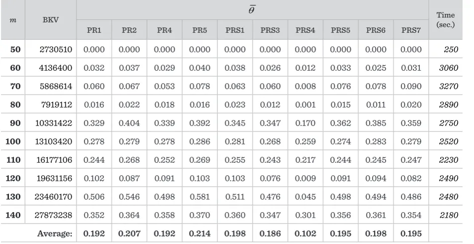
Results of the comparison of different configurations (variants) of HGA (n = 1024) (part III)

m BKV θ Time _(sec.)

PR1 PR2 PR4 PR5 PRS1 PRS3 PRS4 PRS5 PRS6 PRS7

50 2730510 0.000 0.000 0.000 0.000 0.000 0.000 0.000 0.000 0.000 0.000 250

60 4136400 0.032 0.037 0.029 0.040 0.038 0.026 0.012 0.033 0.025 0.031 3060

70 5868614 0.060 0.067 0.053 0.078 0.063 0.060 0.008 0.076 0.078 0.090 3270

80 7919112 0.016 0.022 0.018 0.016 0.023 0.012 0.001 0.015 0.011 0.020 2890

90 10331422 0.329 0.404 0.339 0.392 0.345 0.347 0.170 0.362 0.385 0.359 2750

100 13103420 0.278 0.279 0.278 0.286 0.281 0.268 0.259 0.274 0.283 0.279 2520

110 16177106 0.244 0.268 0.252 0.269 0.255 0.243 0.217 0.244 0.245 0.247 2230

120 19631156 0.102 0.087 0.091 0.103 0.103 0.076 0.009 0.091 0.094 0.082 2490

130 23460170 0.506 0.546 0.498 0.581 0.511 0.476 0.045 0.498 0.494 0.486 2480

140 27873238 0.352 0.364 0.358 0.370 0.360 0.347 0.301 0.356 0.361 0.354 2180

We found out that the following configurations (vari-ants) are quite efficient: IP3, S3, C1, C3, C5, C8, NOG2, NOG3, NOG4, LI3, PR3, PR4, PRS4.

Based on these promising configurations, we have de-signed another 8 algorithmic configurations, which intermix the available algorithm components in pre-viously unexamined ways10_:

1) S3-LI3, 2) S3-C1-LI3-PRS4, 3) S3-NOG3-LI3-PRS4,

4)  S3-C1-NOG3-LI3-PRS4, 5)  S3-C3-NOG3-LI3-PRS4, 6)  S3-C5-NOG3-LI3-PRS4, 7)  S3-C8-NOG3-LI3-PRS4,

8)     S3-C8-NOG4-LI3-PRS4.

Remind that we use the short syntax. For example, S3-LI3 ≡ _IP3, S1, C2, NOG2, LI1, PR3,

PRS2 \ _S1 \ _LI1 ∪ _S3 ∪ _LI3, and so on. The results of these new composed configurations are summarized in Tables 9 and 10.

The results of experiments provide strong evidence that the initial population construction is one of the most important components of HGA (not counting the local improvement). The conclusion is that the quality of the initial population should be as high as possible. Improved and extra-improved populations are clearly preferable to random or low-quality initial populations despite the fact that the smaller number of generations is adopted in the case of improved ini-tial population.

The selection component influences the behaviour of HGA less than the remaining components according to our analysis.

Regarding the crossover operators, it is of high impor-tance that these operators respect the problem-spe-cific information of the problem at hand. The main conclusion is as follows: the specific crossover op-erators are preferable to general-purpose crossover procedures, or at least they are very good alternative ways to the canonical operators. Also, it is observed that good crossover procedures not only include re-combination of genes, but also greedy like or fast local search operations, which enable to obtain the partial-ly optimized offspring already at the stage of recombi-nation of the parents’ genetic material.

There is no straightforward answer as to the number of offspring per generation. Despite the analogy of

10  We present the results of these particular configurations be-cause the results of other tried configurations are of lower quality.

natural behaviour, many offspring are not necessary in the GA. Maintaining a single or few offspring has its advantage in that the updating of the population occurs more rapidly, which helps the speeding up of the evolution process.

It is also shown that the local improvement process, along with the related numerical parameters, is in-deed of the highest importance for HGA. The pro-longed extensive improvement (more iterations of the improvement algorithm) is deemed to have greater potential as compared to the quick, concentrated im-provement (less iterations of the improvement algo-rithm) for a fixed CPU time budget. The values of the parameters Qhier and τ should be carefully calibrated

to achieve the best desirable effect (here, Q_hier denotes the total number of iterations of the hierarchical im-provement algorithm, τ is the number of the TS iter-ations). Overall, it is recommended that the value of the ratio hier

gen

Q

N (or Ngen

τ _{) be large enough (given that}

hier gen

Q ⋅N =const), where N_gen is the number of gen-erations of HGA. (For example, Qhier =100, Ngen =50 would be better than Qhier = 50, Ngen =100.) We

ob-served that the solution quality is more sensitive to the value of τ than Q_hier (if other conditions remain unchanged). So, larger values of τ are recommended, especially if the problem size n is also large.

We notice that the problem-specific, tuned local op-timizer should be adopted to save the computation time.

More attention should be paid to the design and im-plementation of the population replacement compo-nent. It is worth to try new non-traditional replace-ment schemes. Not only the fitness of the individuals is important, but also the distance between popula-tion members. The variability of the individuals of the population must be ensured.

Table 9

Results of the comparison of different configurations (variants) of HGA (n = 256) (part IV)

m BKV

θ

Time (sec.)

S3-LI3 S3-C1-LI3-

PRS4 S3-

NOG3-LI3- PRS4

S3-C1- NOG3-LI3- PRS4

S3-C3- NOG3-LI3- PRS4

S3-C5- NOG3-LI3- PRS4

S3-C8- NOG3-LI3- PRS4

S3-C8- NOG3-

LI3-PRS4♣

S3-C8- NOG3-LI3-

PRS4♣♣

S3-C8- NOG4-

LI3-PRS4♣♣

95 48081112 0.000 0.000 0.000 0.000 0.000 0.000 0.000 0.000 0.000 0.000 200

96 49182368 0.049 0.035 0.021 0.000 0.000 0.035 0.007 0.000 0.000 0.007 450

97 50344050 0.000 0.000 0.000 0.000 0.000 0.000 0.000 0.000 0.000 0.000 210

98 51486642 0.037 0.030 0.015 0.000 0.000 0.000 0.000 0.000 0.000 0.000 230

99 52660116 0.044 0.052 0.035 0.000 0.021 0.040 0.012 0.017 0.013 0.003 550

100 53838088 0.051 0.058 0.052 0.042 0.023 0.029 0.015 0.011 0.016 0.016 610

101 55014262 0.076 0.059 0.059 0.036 0.035 0.030 0.024 0.019 0.024 0.015 610

102 56202826 0.059 0.063 0.064 0.045 0.045 0.050 0.027 0.032 0.041 0.027 740

103 57417112 0.031 0.026 0.026 0.026 0.026 0.026 0.015 0.021 0.023 0.018 600

104 58625240 0.021 0.021 0.021 0.018 0.021 0.019 0.011 0.013 0.013 0.015 540

Average: 0.037 0.034 0.029 0.017 0.017 0.023 0.011 0.011 0.013 0.010

♣ _{enlarged initial population is used (}

1 3 C = );

♣♣ _{enlarged number of tabu search iterations is used (τ =200).}

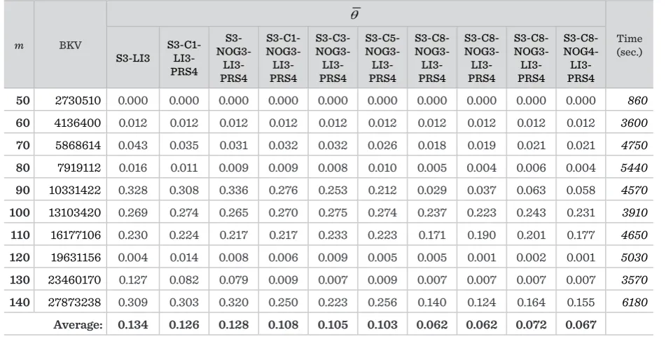
Table 10

Results of the comparison of different configurations (variants) of HGA (n = 1024) (part IV)

m BKV

θ

Time (sec.)

S3-LI3 S3-C1-LI3-

PRS4 S3-

NOG3-LI3- PRS4

S3-C1-NOG3- LI3- PRS4

S3-C3- NOG3-LI3- PRS4

S3-C5- NOG3-LI3- PRS4

S3-C8- NOG3-LI3- PRS4

S3-C8- NOG3-LI3- PRS4

S3-C8- NOG3-LI3- PRS4

S3-C8- NOG4-LI3- PRS4

50 2730510 0.000 0.000 0.000 0.000 0.000 0.000 0.000 0.000 0.000 0.000 860

60 4136400 0.012 0.012 0.012 0.012 0.012 0.012 0.012 0.012 0.012 0.012 3600

70 5868614 0.043 0.035 0.031 0.032 0.032 0.026 0.018 0.019 0.021 0.021 4750

80 7919112 0.016 0.011 0.009 0.009 0.008 0.010 0.005 0.004 0.006 0.004 5440

90 10331422 0.328 0.308 0.336 0.276 0.253 0.212 0.029 0.037 0.063 0.058 4570

100 13103420 0.269 0.274 0.265 0.270 0.275 0.274 0.237 0.223 0.243 0.231 3910

110 16177106 0.230 0.224 0.217 0.217 0.233 0.223 0.171 0.190 0.201 0.177 4650

120 19631156 0.004 0.014 0.008 0.006 0.009 0.005 0.005 0.001 0.002 0.001 5030

130 23460170 0.127 0.082 0.079 0.009 0.007 0.009 0.007 0.007 0.007 0.007 3570

140 27873238 0.309 0.303 0.320 0.250 0.223 0.256 0.140 0.124 0.164 0.155 6180