Automatic Determination of Skeletal Maturity using Statistical Models of Appearance

Automatic Determination of Skeletal Maturity

using Statistical Models of Appearance

Steve A. Adeshina, Timothy F. Cootes, and Judith Adams.

Abstract—This work addresses the problem of automatic determination of skeletal maturity in children and young adults. Skeletal age assessment is important for diagnosing and monitoring growth and endocrine disorders. We have constructed a system which uses Statistical Models of Shape and Appearance to locate bones in a radiograph and to predict skeletal maturity. By analysing the performance on a dataset of about 600 digitised radiographs of normal children we show that different variants of Part+Geometry (P+G) models are sufficient to initialise an automatic registration algorithm. We built global models of whole hand and local models of individual bones. We used the same P+G models to locate salient bones of the hand to initialise an Active Appearance Model (AAM) to match all the bones of the hand in a radiograph. We improved our age estimation results by using multiple local age group models and multiple local age estimators. We obtained an accuracy of0.75mmand0.70mmon sparse points placement for initialization of automatic registrations and Active Appearance models fitting respectively. We achieved a sub-millimeter accuracy for automatic model annotation and for locating the bones in a new radiograph. Our skeletal maturity methodology achieved an accuracy in estimating Skeletal Age of mean absolute error of0.41±0.02years and0.47±0.03years for female and male respectively.

Index Terms—Skeletal maturity assessment, Constrained Active Appearance Models, Part-based Models

F

1

I

Skeletal age assessment is an important non invasive routine procedure which is based on the observation of the X-ray image of the non-dominant hand. A significant difference in the bone age and the actual age of a child is an indication of growth abnormalities. Skeletal assessment is used in the diagnosis and management of growth and endocrine disorders in children and young adults [24]. The assessment helps in determining ulti-mate adult height in children and young adults and in planning orthopaedic procedure involving the vertebrae column [25], [17].

The two main methods used are based on the obser-vation of bone morphology from a radiograph of the non-dominant hand. Though there are other attempts at assessing skeletal maturity from other parts of the body, (Pyle and Hoer (1969) based their method on the analysis of the knee [17]), the methods attributed to Greulich and Pyle(GP) [17] and Tanner and Whitehouse(TW2/3) [25] have remained dominant in the assessment of skeletal maturity in clinical radiology. The GP method is very highly subjective, while the TW 2 method is less sub-jective but time consuming. They are both subjected to inter- and intra- observers variability. These constitute our motivation for this work.

Although there has been a great deal of efforts in de-termining skeletal maturity of children and young adult using several automated methods [21], [23], the

appli-• Dr Steve Adeshina is with the Department of Electrical and Electronics Engineering, Nile University of Nigeria, Abuja, Nigeria.

E-mail: [email protected]

• Prof Timothy Cootes and Prof Judith Adams are with Centre for Imaging Sciences, The University of Manchester, U.K

cation of Statistical models in this domain is relatively new. In this work we demonstrate that use of Statistical models appearance and Parts and Geometry models to automatically annotate Radiographs of children and young adults. We built Statistical Models of whole hand image and of several bone complexes of the hand. By fitting these models to images of oncoming radiograph we were able to estimate skeletal age using multiple linear regressors and the Tanner and Whitehouse (TW3) readings as ground truth.

We demonstrate that our approach outperforms al-ternative skeletal maturity determination methodology across several application areas, achieving what we be-lieve to be one of the best results yet published in the literature. Additionally we also automated the process of building statistical models - a very tedious and time consuming process.

2

R

W

the borders of 15 bones automatically and computed intrinsic bone ages for each of the 13 bones (radius, ulna and 11 short bones). They transformed the intrinsic bone ages into TW and GP bone ages [28].

Mahmoodi et al.[19] and Volgesanget al. [31] used a knowledge based modeling method for the assessment of skeletal maturity. Cao, Pietka and Gilanz [10] pro-posed a digital hand atlas and a web-based bone age as-sessment system. Taaniet al.[7] utilized a Point Distribu-tion Model (PDM) to determine skeletal maturity. Pietka et al. [23] describe a Computer-assisted bone age assess-ment method, which is a classical image (pixel) level processing of a Region of Interest (ROI). A population based approach to bone age using the TW3 as knowledge base was proposed by Zhaoet al.[33] recently. Giordano et al. [16] developed an automated system for bone age assessment. Bocchi and his co-workers [9] recently implemented a method to determine bone age with the Artificial Neural Network(ANN) using the TW2 method. Tristan and Arribas [29] in their “Radius and ulna skeletal age assessment system” proposed a method to automate the TW3 skeletal assessment method using K-means algorithm for segmentation. Recently Zhang et al. [32] use classical image processing technique to automatically extract the Carpal bones of children from 0 - 7 years.

The most closely related work to that presented here is that of Thodberg et al.[28], who showed how Active Appearance Models [13], [27] can be used to locate the bones of the hand and how the parameters of the associated appearance models can be combined with other texture measures to predict skeletal age. Whereas Thodberg et al. used models of the individual bones, we build local appearance models of the regions around the bones and joints. Their model building process is fully manual while we introduced automatic registration of the bones during the model building process. While they estimated ages from fifteen bones we estimated ages from all the bones to get the optimal combination of bones.

We have used appearance (a combination of shape and texture) as an entity to determine skeletal maturity. We used the entire 13 bone complexes consistently for the prediction of skeletal maturity. The introduction of an automatic registration method for building of local models and the use of appearance parameters are the key contribution of this work. Our results competes positively with Thodberg’s [28] and ranks amongst the best in this application domain in the literature.

In our approach we sparsely annotated the digitized radiograph images to describe the entire bones of the hands using Parts based models. We then extracted 20 bone complexes and each complex was automatically registered. Appearance models were built for each of the extracted complexes. These models were fitted to images using multiple linear regressors to estimate skeletal ma-turity for each of the bone complexes. Predicted ages were obtained for each of the complexes and averaged

for the 13 RUS bones complexes to obtain bone age for each radiograph. Figure 1 shows maturity growth points used and some local models of bone complexes. In the following section we describe the overview of the entire system.

(a) (b)

Fig. 1. (a) Skeletal maturity growth points based on TW method.RUS bones:Radius(1), Ulna(2), Metacarpal I, III, V, Proximal phalanges(ppha) I, III, V (10,15,16) , Middle phalanges (mpha) III, V (14,17), Distal phalanges (dpha) I, III, V (12,13,18);Carpal bones:Capitate(4), Ha-mate(5), Triquetral(8), Lunate(3), Scaphoid (8), Trapez-ium(6) and Trapezoid(9).

(b)bones of the hand [1]

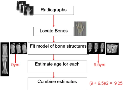
2.1 Skeletal maturity Determination - Overview Given a set of radiographs whose skeletal ages we wish to determine, we use models of the whole hand to locate the approximate position of the bones, then fit models of the different bone structures and extract parameters of the models from each structure. We use the extracted parameters to estimate age for each bone structure. We then combine these estimates by averaging over all the bone structures.

Figure 2 shows the overview of our proposed system.

3

M

We have access to a database of radiographs of the non-dominant hand of normally developing children being collated by the University of Manchester. Their ages ranged between 5 years and 19 years. In the following work we used a subset of 644 digitized radiographs of normal children. The images were divided into three groups of ages 5-7 (66 images), ages 7-13 (335 images) and ages 14-18 (243 images) years.

3.2 Part Based Models

In earlier work we described how Part based Models are built [2]. For our purpose we start by Initializing a model with a set of boxes; then Automatically define a set of arcs; Build a P+G model of one example; Use model to find matches in dataset; Rank result by final fit value; Build P+G models from 50% of matches; Iterate. The matching algorithm thus seeks to find the candidates which minimise the following function

F =

N X

i=1

fi(gi) +α X

(i,j)∈Arcs

fij(pi,pj) (1)

where the first items represent the function of the intensity of the Patch model and the second item rep-resent the second item reprep-resents the geometrical rela-tionship between the patches. The value of αaffects the relative importance of patch and geometry matches. In the following we use α = 0.1, chosen by preliminary experiments on a small subset of the data. For details please see [2]

3.3 Building the Model

We initialise a model using a set of parts defined by boxes placed on a single image by the user (for instance, the rectangles shown in Figure??a). This takes about one minute to do, and allows the algorithm to take advan-tage of user supplied knowledge. We then automatically define a set of connecting arcs based on the distances between the centres of the boxes. We use a variant of Prim’s algorithm for the minimum spanning tree, where each node has two parent nodes, rather than one [8].

We then refine the model by applying it to the whole dataset, ranking the results by final fit value (per image), and building statistical models of intensity and pairwise relationship from the best 50% of the matches.

3.4 Construction of Statistical Appearance Models

Statistical appearance models (SAM) [13] were generated by combining a model of shape variation with a model of texture variation. Each radiograph was manually anno-tated with points around important structures. Statistical models of shape and texture (intensities in the reference

frame) were constructed by applying Principal Compo-nent Analysis (PCA) to the resulting annotations, leading to linear models of the form

x= ¯x+Psbs g= ¯g+Pgbg (2)

where x¯ is the mean shape, g¯ is the mean texture,

Ps,Pgare the main modes of shape and texture variation and bs,bg are the shape and texture model parameter vectors. Combining the shape and texture models gives a combined appearance model of the form

x= ¯x+Qsc g= ¯g+Qgc (3)

whereQs,Qgare matrices describing the modes of vari-ation derived from the training set andcis a combined vector of appearance parameters controlling both shape and texture.

3.5 Groupwise registration

The sparse annotation uses only a few points for each local bone complex model, so does not represent de-tails of the bone shape. To improve the density of the correspondences we applied a ‘groupwise’ non-rigid registration algorithm, similar to that in [12], initialised with the manual points. For each structure we defined a dense triangulated mesh on one image, then used the sparse annotation from PBM to propagate this to the other images using thin-plate spline interpolation. We then estimated the mean shape and texture and applied a non-rigid registration approach to improve the correspondence between each image and the mean. The process is repeated until convergence, leading to an accurate, dense correspondence across the set. Models of shape, texture and appearance were then constructed from the resulting points.

3.6 Active Appearance Model search

The AAM matching algorithm is outlined below. There are two main components: a parameterized model of ob-ject appearance, and an estimate of relationship between parameter errors and image residuals [11].

The appearance model parameters,c, and shape trans-formation parameters,t, define the position of the model points in an image frame, X, which gives the shape of the image patch to be represented by the model. During the matching we sample the pixels in the region of the image,gimand project them to the texture model frame,

gs = T−1(gim). The current texture model is given by

gm = ¯g+PgQgc The model, image difference in the normalized texture frame is

r(p) =gs−gm (4)

r(p+δp) =r(p) + ∂r

∂pδp (5)

where the ijthelement of matrix ∂r

∂p is

dri

dpj

If our current residual is r, we intend to choose δp

so as to minimize |r(p+δp)|2 by equating equation 5 to zero, we then get a Root Mean Square solution as shown below:

δp=−Rr(p) where R=

_∂rT

∂p

∂r

∂p

−1_∂rT

∂p (6)

It would be necessary to re-calculate ∂r

∂p in standard

optimization exercise and this is computationally expen-sive. It is however considered approximately fixed - the estimation can be done from the training set. Numeric differentiation can be used to estimate ∂r

∂p displacing

each parameter systematically from the known optimal value on typical images and computing the average over a set. Residuals at displacements of differing magnitudes measured - say 0.5SD for each parameter and this is combined with a Gaussian to smooth them. R is pre-calculated and used for subsequent searches [11]. The images used in calculating the partial residuals can be examples from the training set or the images generated using the appearance model.

3.7 Constrained active appearance models (CAAM) The AAM as a local search method depends on an update matrix learned near correct solutions. As a result, it depends upon adequate initialisation. Usually this initialisation is provided by prior estimates of some of the shape points, either manually, or through automatic methods as discussed in preceding sections. There may be some prior knowledge of the variances associated with these initialisation points. Cootes et al. developed the Constrained AAM [14] to incorporate such con-straints.

Essentially the least squares minimisation of the stan-dard AAM is replaced by a maximum a-posteriori (MAP) formulation, which seeks to maximise the prob-ability of the model given the data which (by Bayes theorem) is proportional to:

P(data|model)P(model) (7)

Assuming a uniform prior on the model parameters. This can be equated to a least squares formulation where Gaussian residuals are not correlated and the variances are equal. A Gaussian prior could be assumed on the model parameters, and Cootes et al. showed how the AAM update step can be reformulated to incorporate this prior. In the rest of this section we will be concentrat-ing on incorporatconcentrat-ing prior knowledge about constrained points. We worked with a simplified version of [14] and assumed a constant model prior [1].

The Jacobian of the residual can be represented as J

(see section 3.6)

J= δr

δp (8)

as a result equation 6 in section section 3.6 can be re-written as

R=

JTJ−1

JT (9)

Suppose we have prior estimates of the positions of some points in the image frameX0, together with their covariance matrix SX. Unknown points can be repre-sented by zeroes, together with large upper bounds in

SX, and effectively zeroes inSX−1. Letd(p) = (X−X0) be a Vector of the displacements of the current point positions from their prior positions. We assume further that the prior point positions are Gaussian distributed, and also that the texture residuals are independently and identically distributed with varianceσr2_{.ris the Vector} of residuals. Then maximising the logarithm of the MAP is equivalent to minimising (see section 3.6):

E1(p) =σr−2rTr+dTSX−1d (10)

By using a first order Taylor expansion similar to that used to derive the basic AAM update equation, the parameter update is given by the solution to the equation set:

Aδp=−a (11)

where, after defining the Jacobian ofdw.r.tpasK

A = σr−2JTJ+KTSX−1K

a = σr−2JTr(p) +KTSX−1d

(12)

and

K= δd

δp (13)

When computing the prior point displacement Jacobian K, it is necessary to take into account the global pose transformation t as well as the appearance model parameters c. Cootes further developed the special case of isotropic prior point positional variance with zero off-diagonal terms, and when the pose transformation St(x) is a similarity transform which scales by s. Letx0 be the prior point positions mapped into the model frame, so x0 = St−1(X0), and let

y=s(x−x0). ThendTSX−1d=yTSX−1y.

In this case:

A = σr−2JTJ+KmTSX−1Km

a = σr−2JTr(p) +KmTSX−1y

(14)

The JacobianKmis the concatenation _δy

δc|

δy

δt

and:

δy

δc = sQs

δy

δt = −s

δ St−1(X0)

δt −(x−x0)· _sx

s , sy

s ,0,0

3.8 Estimation of skeletal maturity

Given the appearance models we can compute shape, texture and appearance parameter vectors for each struc-ture on each image.

We use classical linear regression of the form, A = wT_p+A

0, whereAis the predicted age,wis a vector of weights,pis the parameter vector andA0is a constant. In the following we describe experiments comparing the performance of different models of the carpal bones [1].

4

E

R

In our earlier works we performed experiments to deter-mine the required optimal number of bones, the type of models, the most effective parameters amongst others [6]. The following are the conclusions derived from the experiments and they actually formed the basis of further experiments.

• That global hand models perform poorly when

com-pared with local ones in skeletal age estimation.

• That improvements in accuracy can be achieved

by using models of the joint complexes and bones constructed by automatic registration, compared to those built from manual annotation as in table ??.

• _{Appearance parameters correlate with skeletal}

ma-turity better than shape or texture features alone.

• The Carpal bones seem to contribute negatively to

the estimation of skeletal maturity.

• The results also show that the 13 bones complexes

of Radius, Ulna and Short bones are sufficient to estimate bone age.

• That good predictions of Chronological Age can be

made using simple linear predictors based on the parameters of appearance models of bones and joint complexes of the hand as earlier shown in [28].

• That a series of linear predictors may perform better

than a single linear predictor.

• _{That Chronological Age may not be the best}

predic-tor of skeletal age.

• _{These results also confirms what was described in}

the literature.

4.2 Major earlier experimental works

The block diagram in Figure 2 requires that we anno-tate training radiographic image before we can build models. Initially we manually annotated images but the process was ultimately automated, with very minimal manual intervention. It was also very important to locate salient landmarks on the radiographs. This process will be useful, both as an initialization for the automatic annotation of the Radiograph and for model matching to ensure that the Models do not collapse into a local minimum. The parts and Geometry models was key to achieving the proceeding requirement. Locating the bones and building global and local models of the hand is a direct consequence of identifying salient points on

the hand. We briefly discuss the following published experimental works.

• Constructing part based models for groupwise

reg-istration [2]

• Automatic Annotation of Radiographs using part

and Geometry model for building statistical models for skeletal maturity [3].

• Automatic model matching using part based mode

constrained active appearance models [4]

• Automatic determination of skeletal maturity using

statical models of appearance [1]

4.2.1 Constructing part based models for groupwise registration

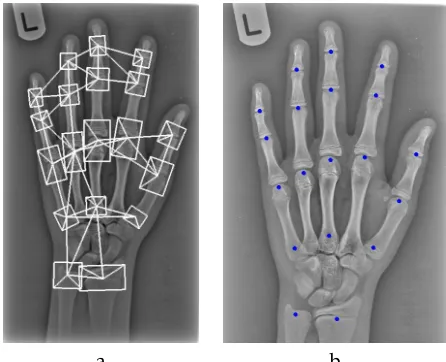
This section addresses the problem of building detailed models of the shape and appearance of complex struc-tures, given only a training set of representative im-ages and some minimal manual intervention. Using a sparse annotation of a single image we can construct a parts+geometry model capable of locating a small set of features on every training image. Iterative refinement leads to a model which can locate structures accurately and reliably. The resulting sparse annotations are suffi-cient to initialise a dense groupwise registration algo-rithm, which gives a detailed correspondence between all images in the set. We demonstrate the method on a large set of radiographs of the hand, achieving less than 1 millimeter accuracy. With this method we are able to locate automatically 19 major landmarks on the hand radiograph. Figure 3 shows a typical Part Based Model and the located 19 points. These major points becomes very useful in initial annotation and building of original models and initialization of unseen radiograph for automated model matching. Further details on this can be found in [2]

a b

4.2.2 Automatic Annotation of Radiographs using part and Geometry model

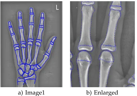
Statistical Models of Shape and Appearance require annotation of the bones of the hand of children and young adults. Due to very large variation in the shape and appearance of these bones, automatic annotation is particularly challenging. In this experiment we built a semi-automatic Parts and Geometry model to locate sparse points in each of the Radiographic image. These sparse points were then used as control points to propa-gate densely manually annotated points on one image to other images. The resulting propagation was used to build Statistical models that have be found to be useful in estimating skeletal maturity. By analysing per-formance on dataset of 537 digitized images of normal children we achieved an automatic annotation accuracy of a mean point to curve error of 1mm±0.08 and a median error0.94mm. Automatic annotation reduces the need for tedious manual annotation. The resulting anno-tated images were subsequently used to build global and local models. Suffice it to say here that, these annotation process also allows us to separate the radiograph image into the constituent bones and bone complex that are required for building Local models. For further details please see [5]

a) Image1 b) Enlarged

Fig. 4. Quantitative results of propagation of 2,797 points based on the Part based models’ automatic initialization for two examples in group 3

4.2.3 Automatic model matching using PBM Con-strained Active Appearance Models for skeletal maturity

One critical requirement in automated skeletal maturity estimation is matching built models to unseen images of the bones of the hand. Oftentimes some form of ini-tialization is required to prevent the model from falling into local minima. In this experiment [4]we used part-based models to initialize the image of an incoming radiographic image and then fit a global Active Appear-ance models of the whole hand using the found points from the Part based models as ’weighted’ constraints. Having found the approximate positions of the bones of the hands we then fit local models to refine the model

fit. By analysing performance on our dataset of digitized images of normal children we achieved a model fitting accuracy of an overall point to point median error of

0.7mm. Figure 5 shows stages required for matching an unseen radiographic images. This is to ensure each bone is located for subsequent matching which models that were already built. For details please see [4].

Fig. 5. Process flow for CAAM fit. From 19 automatically found points on 94 images, 330 manual points on a reference image, a TPS warp of manual points to other images, a further refine fit and final points’ result.

4.3 Estimating Skeletal maturity from model param-eters

Statistical appearance models [13], [15] were generated by combining a model of shape variation with a model of texture variation. Each radiograph was automatically annotated with 19 points around important structures. The sparse 19 points were used to densely annotate each Radiograph. Statistical models of shape and texture (intensities in the reference frame) were constructed by applying Principal Component Analysis (PCA) to the resulting annotations, leading to linear models of the form

x= ¯x+Psbs g= ¯g+Pgbg (16)

wherex¯ is the mean shape,g¯is the mean texture,Ps,Pg are the main modes of shape and texture variation and

bs,bgare the shape and texture model parameter vectors. In addition a combined model is constructed

x= ¯x+Qsc g= ¯g+Qgc (17)

whereQs,Qgare matrices describing the modes of vari-ation derived from the training set andcis a combined vector of appearance parameters controlling both shape and texture.

By matching these models to each structure in each image, we can extract the relevant model parameters.

A=wTp+A0 (18)

where Ais the Predicted Age, w is a vector of weights,

pis the vector of parameters (eitherbs,bg,c) andA0is the intercept constant.

Images as shown in Table 1 were automatically anno-tated as described above. Shape, texture and appearance models were built.

For each model we computed the shape, texture and appearance parameters for every image. We then eval-uated the utility of linear age prediction models using a Leave-One-Out (LOO) paradigm. We trained linear regressors to predict age on all but one image, then tested the prediction on the left-out image. Since male and female children are known to develop at different rates, different regressor models were used for the male and the female sets. We evaluated performance using the mean absolute error between prediction and Chronolog-ical Age.

Preliminary experiments published in earlier work [6] show that a set of models representing local structures of the bone performs better than a single model. In this regard we used several models of different bone structures.

We improved the overall age prediction by averaging the ages estimated from each local bone model over the set (Aµ= _n1PN

i=1Ai, whereAiis the prediction from the ith_{local model).}

4.4 Predicted Age with Chronological Age

The goal of these experiments is to compare predicted age with chronological age in this cohort of normal children. Though chronological age is not the best pre-dictor of skeletal age, there is a reasonable relationship for normal children. The GP atlas was based on the assumption that the chronological age is equal to skeletal age for normal children.

We used the same experimental protocol as for pre-liminary experiments, but being a larger data set, broken down by age range.

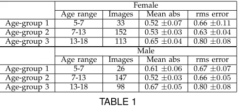
These experiments were performed for each of the 13 bone complexes in each of the three groups. The predic-tions were averaged over the 13 RUS bone complexes. Table 1 show the mean absolute errors and the root mean square errors for the three age-groups.

Figure 6 shows the scatter plots for the three age-groups. The plots confirm the earlier hypothesis that chronological age correlate with bone age. However the spread around each line is about ±1 year. This shows that skeletal age is not the best predictor of chronolog-ical age. However it shows that the choice of multiple predictors is useful. We explore further by using expert TW3 readings as will be shown in the next section.

4.5 Predicted Age with expert TW3 readings.

The motivation for the experiment is to investigate the performance of linear predictors using expert TW3

read-Female

Age range Images Mean abs rms error Age-group 1 5-7 33 0.52±0.07 0.66±0.11

Age-group 2 7-13 152 0.53±0.03 0.63±0.04

Age-group 3 13-18 113 0.65±0.04 0.80±0.08

Male

Age range Images Mean abs rms error Age-group 1 5-7 26 0.61±0.06 0.67±0.07

Age-group 2 7-13 147 0.52±0.03 0.66±0.05

Age-group 3 13-18 98 0.67±0.05 0.80±0.08

TABLE 1

Mean absolute predictions error (years), root mean square (rms) error (years) and number of images, using

Chronological Age as the ground truth

ings. Most methods for estimating skeletal maturity use expert TW3 readings as ground truth. This experiment compares our result with what is published in the liter-ature [26]. At the conception of this project, the expec-tation from the clinical radiologists was to simply auto-mate the process of TW3 reading. By performing these experiments, we show that it is possible to predict age by training linear predictors with expert TW3 readings. Our result compares favorably with other published method in this regard.

We have access to TW3 expert readings1_{for about 450}

images. We used the final computed age for each image. We performed a similar experiment to that described in Section 4.4 but used the final predicted TW3 ages to train the linear predictors. However, some of the images are above chronological age of 18 years. Observation of the data shows that every image with chronological age of 15 years and above for female were estimated as adult and scored at the maximum skeletal age of 15 years. For male the maximum skeletal age scored is 16.5 years. We excluded images around these extremes as our linear estimators would have been confused if chronological ages from 15 - 18 years are equated to skeletal age of 15 years during training for female and chronological ages from 16.5 - 18 years are equated to skeletal age 16.5 years for male.

The limit for scoring of bone age in the TW system is 5-15 years for female and 5-16.5 years for male [26]. The limit of bone age estimation for the GP method is 0-18 years for male and female [17]. This is however very subjective, being an atlas based system, where chronological age is equated to skeletal age.

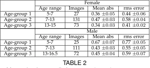
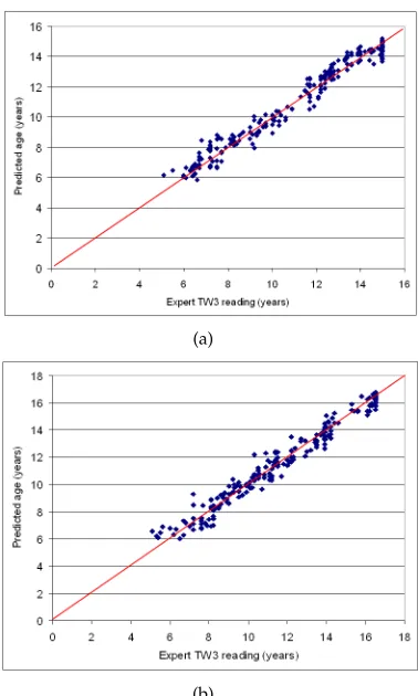
Table 2 show the mean absolute prediction errors, the root mean square errors and the number of images used. Figure 7 shows the plots of expert TW 3 final age reading against Predicted Age for male and female. The predictions is better than that of chronological age may have been limited by the upper limit of 15/16.5 years for female and male respectively. It is believed that these limitations are imposed as a result of the limitations of what the human eye can see. An age prediction

Female

Age range Images Mean abs rms error Age-group 1 5-7 27 0.36±0.05 0.44±0.06

Age-group 2 7-13 131 0.47±0.03 0.58±0.04

Age-group 3 13-15 73 0.34±0.03 0.41±0.02

Male

Age range Images Mean abs rms error Age-group 1 5-7 25 0.67±0.07 0.77±0.05

Age-group 2 7-13 111 0.43±0.03 0.55±0.05

Age-group 3 13-16.5 72 0.45±0.04 0.59±0.07

TABLE 2

Mean absolute predictions error (years), root mean square (rms) error (years) and number of images, using

TW 3 expert readings as the ground truth

system can potentially go beyond these limits. Though we we thought in [1] that developing a system purely on one or two raters’ reading is not ideal. However, with further introspection, we now believe that a model can generalize to images it has not seen as examples. We advice the use of Chronological age as a substitute for the TW3 and suggested to our Expert to read the ’left out’ range with GP atlas.

4.6 Predicted Age with Consensus Skeletal Age

In line with the thought of Thodberget al.[28] we inves-tigate a new maturity measure that does not depend on the readings of the experts.

They believed that there are inherent properties of different bone complexes represented by the extracted features that correlate with maturity. To ensure that the children in this study are normal, continuous medical tests and investigations are carried out on a regular basis. For this reason, the normality of the children can be as-sumed and we could rely on chronological age in a way that emphasises those image features that are related to maturity rather those that relate to Chronological age [28]. This they achieved using the concept of Consensus Skeletal Age.

Similar experiments were performed as in preceding sections. Observation of the predictions from chrono-logical age shows that the predictions for the 13 bone complexes have minimal differences. This reflects the differences in the development of the bone complexes. The development of the bone complexes tend to com-plement for each other. We therefore postulate that there is a value for the skeletal age which has a relationship with chronological age. This value tends to be around that predicted based on chronological age. Since we have predictions from 13 complexes we simply average the values and used these average values (Consensus Skeletal Age) to train our regressor. This approach was first introduced by Thodberget al.[28]. We differ slightly in our approach. Based on medical studies, a number of complexes are considered necessary and sufficient for bone ageing. This is because the development of these bones are considered to be complementary [26]. The

redundancy based on synchronous development seem to have been compensated for by reducing the numbers of complexes to 13 in TW system. The TW system and the GP system assess 13 and 28 bones respectively [26], [17]. We believe any reduction below this number may lead to losing vital information about the bone age of the individual. We therefore adopted a consistent averaging of values as opposed to Thodberg’s where they set a threshold of acceptable predictions from each bone complex and a minimum threshold of at least 7 complexes before age can be estimated from the image. Table 3 and Figure 8 show results obtained by using the Consensus Skeletal Age. We will refer to this Pre-dicted Age as Intrinsic Skeletal Age.

Female

Age range Images Mean abs rms error Age-group 1 5-7 33 0.15±0.02 0.20±0.01

Age-group 2 7-13 152 0.12±0.01 0.14±0.002

Age-group 3 13-18 113 0.2±0.01 0.24±0.01

Male

Age range Images Mean abs rms error Age-group 1 5-7 26 0.28±0.04 0.34±0.03

Age-group 2 7-13 147 0.15±0.01 0.18±0.003

Age-group 3 13-18 98 0.16±0.01 0.20±0.01

TABLE 3

Mean absolute prediction error (years), root mean square (rms) error (years) and number of images, using

Consensus Skeletal Age as the ground truth

Female

Images Mean abs rms error Chrono Age 298 0.57±0.02 0.70±0.04

Consensus Age 298 0.15±0.01 0.19±0.002

Expert TW3 231 0.41±0.02 0.52±0.03

Male

Images Mean abs rms error Chrono Age 271 0.58±0.03 0.72±0.04

Consensus Age 271 0.16±0.01 0.21±0.004

Expert TW3 208 0.47±0.03 0.59±0.04

TABLE 4

Mean absolute prediction error (years), root mean square (rms) error (years) and number of images. Predictions from Chronological Age, Consensus Skeletal

Age and TW3 readings respectively

.

4.7 Evaluating precision

(a)

(b)

Fig. 6. (a) Consolidated predictions plot (for the 3 groups) from Chronological Age for male and (b) for female. This figure corresponds to table 4

residual (observations)r can be defined as

r=B−(A+C)/2 (19)

The precision errorecan then be estimated from a set of observations of r

e=rms(r)/√1.5 (20)

where rms is the root of the mean of the squares. The derivation of this formula can be found in [28]. We find these values to be similar to the mean absolute difference of the interpolation residuals. These residuals are the difference in years between a set of predicted skeletal ages and the equivalent difference in real ages. The assumption is that the change in Predicted Age is linear with changes in actual actual age. This is not always true especially when the time interval is long. When the increase is non linear, the residual is correspondingly increased. The precision is an upper estimate.

4.8 Precision experiments

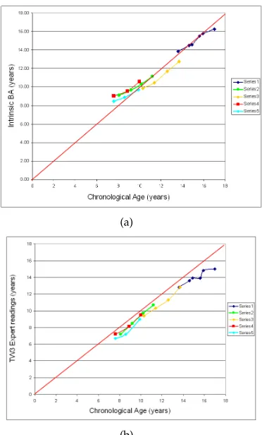
We performed precision experiments by computing In-trinsic Skeletal age for five series of longitudinal images shown in Figures 9a and 9b.

We have 33 observations from the 5 longitudinal se-ries. We derived precision using longitudinal series taken

(a)

(b)

Fig. 7. (a) Consolidated predictions plot (for the 3 groups) from Expert TW3 readings for female and (b) for male. This figure corresponds to table 4

at intervals. We estimated precision using the method described in section 4.7. The precision is estimated to be 0.44 years. We compared these values with equivalent manual TW3 Values and obtained a precision of 0.41 years. The precision value is higher than expected. We think this is attributable to the inconsistencies of the time intervals during which the X-rays of the series were taken. We also think that the non-linearity is introduced as a result of long time intervals. We hope to further study the precision of new longitudinal series.

5

D

C

(a)

(b)

Fig. 8. (a) Consolidated predictions plot (for the 3 groups) from Consensus Skeletal Age for female and (b) for male. This figure corresponds to table 4

in the literature. By achieving a sub-millimeter accuracy for automatic model annotation and for locating the bones in a new radiograph, we can confirm that we revolutionized automatic model building [2]. This use to be tedious and time consuming.

The results from consolidation show mean absolute prediction errors of 0.57 ±0.02 years and 0.58±0.03for female and male respectively. These values are equiv-alent to RMS error of 0.70 and 0.72 years respectively. This result is comparable to that of Thodberg et al.[28] who achieved an RMS error of 0.8 years. This is with respect to predictions based on chronological age. This is the closest work to our work.

Whereas Thodberg et al.built their models manually, an exercise that may have taken several man years, we built ours automatically.

Our precision result of 0.44 years is unsatisfactory for reasons already given, we hope to get new sets of longitudinal data with reasonable time intervals to compute precision. The precision of our manual rater was 0.41 years. Thodberg et al.[28] recorded a precision error of 0.24 years for the optimized validation on TW3 methods. We are constrained not to do this for reasons already stated. However we are concerned about the high level of precision recorded.

(a)

(b)

Fig. 9. (a) Five longitudinal series to determine precision with our system’s Intrinsic Skeletal Age. (b) The same series using TW3 manual readings. Value in section 4.7

Finally Thodberg et al.[28] introduced the concept of Consensus skeletal age which we adopted in [1]. We however now believe that there is no reason why we cannot use the expert readings to estimate Skeletal maturity. The thinking in [28] is that intra- and inter-rater variability is incorporated into the design. Additionally that the limit of about 16.5 years is a limitation. We how-ever believe that a model can generalize to examples that it has not seen and where necessary GP readings should be used to complement the available TW readings at the upper extremes. The work is limited by the age range of 5 to 18 years.

A

The authors would like to thank Lianne Reddie for the TW3 Readings

Steve A. AdeshinaDr Steve A Adeshina is with the Nile University of Nigeria, Abuja Nigera.

Judith Adams is with Centre for Imaging Sciences, The University of Manchester, Manchester, UK.Judith Adams

R

[1] S. A. Adeshina. Automatic Determination of Skeletal Maturity using Statistical Models of appearance. PhD thesis, University of Manchester, 2010.

[2] S. A. Adeshina and T. F. Cootes. Constructing part-based mod-els for groupwise registration. In Proc. 2010 IEEE International Symposium on Biomedical Imaging, pages 733–740, 2010.

[3] S. A. Adeshina and T. F. Cootes. Automatic annotation of radio-graphs using parts and geometry models for building statistical models for skeletal maturity. In Proc. 2014 IEEE International Conference on Electronics Computers and Computation, pages 733– 740, 2014.

[4] S. A. Adeshina and T. F. Cootes. Automatic model matching using part based model constrained active appearance models for skeletal maturity. InProc. 2015 IEEE International Conference on Electronics Computers and Computation, pages 733–740, 2014. [5] S. A. Adeshina and T. F. Cootes. Automatic segmentation of carpal

area bones with random forest regression voting for estimating skeletal maturity in infants. In Proc. 2014 IEEE International Conference on Electronics Computers and Computation, pages 733– 740, 2014.

[6] S. A. Adeshina, T. F. Cootes, and J. Adams. Evaluating different structures for predicting skeletal maturity using statistical ap-pearance models. In J. Dehmeshki, A. Hoppe, and D. Greenhill, editors,Proceedings of the 13th Medical Image Understanding and Analysis Conference, pages 62–66, London, England, 2009. BMVA Press.

[7] A. T. Al-Taani, I. W. Ricketts, and A. Y. Cairns. Classification of hand bones for bone age assessment. InProceedings of the Third IEEE International Conference on Electronics, Circuits, and Systems, volume 2, pages 1088–1091, October 1996.

[8] A.Nonymous. (reference removed to preserve anonymity). In Some Notable Conference, pages xxx–xxx, 0000.

[9] L. Bocchi, F. Ferrara, I. Nicoletti, and G. Valli. An artificial neural network architecture for skeletal age assessment. InProc. 2003 International Conference on Image Processing, volume 1, pages 1077– 1080, Sept. 2003.

[10] F. Cao, H. K. Huang, E. Pietka, and V. Gilsanz. Digital hand atlas and web-based bone age assessment: system design and imple-mentation. Computerized Medical Imaging and Graphics, 24(5):297– 307, 2000.

[11] T. Cootes and C. Taylor. Statistical models of appearance for medical image analysis and computer vision. InSPIE Medical Imaging, Feb 2001.

[12] T. Cootes, C. Twining, V.Petrovi´c, R.Schestowitz, and C. Taylor. Groupwise construction of appearance models using piece-wise affine deformations. In 16th British Machine Vision Conference, volume 2, pages 879–888, 2005.

[13] T. F. Cootes, G. J. Edwards, and C. J. Taylor. Active appearance models.IEEE Transactions on Pattern Analysis and Machine Intelli-gence, 23(6):681–685, 2001.

[14] T. F. Cootes and C. J. Taylor. Constrained active appearance mod-els. In8th_{International Conference on Computer Vision, volume 1,}

pages 748–754. IEEE Computer Society Press, July 2001. [15] T. F. Cootes, C. J. Taylor, D. Cooper, and J. Graham. Active shape

models - their training and application.Computer Vision and Image Understanding, 61(1):38–59, Jan. 1995.

[16] D. Giordano, R. Leonardi, F. Maiorana, G. Scarciofalo, and C. Spampinato. Epiphysis and metaphysis extraction and classifi-cation by adaptive thresholding and d.o.g filtering for automated skeletal bone age analysis. In29th Annual International Conference of the IEEE Engineering in Medicine and Biology Society - EMBS 2007, pages 6551 – 6556, 22-26 Aug. 2007.

[17] W. W. Greulich and S. I. Pyle. Radiographic Atlas of Skeletal Development of Hand Wrist. Palo Alto, CA: Stanford Univ. Press, 1971.

[18] T. S. Levitt, M. W. Hedgcock, D. N. Vosky, and V. M. Shadle. Model-based prediction of phalanx radiograph boundaries. In Proc. SPIE Medical Imaging, volume 1898, pages 670–678, 1993.

[19] S. Mahmoodi, B. S. Sharif, E. Chester, J. P. Owen, and R. Lee. Auto-mated vision system for skeletal age assessment using knowledge based techniques. InImage Processing and Its Applications, 1997., Sixth International Conference on, volume 2, pages 809 – 813, July 1997.

[20] S. Mahmoodi, B. S. Sharif, E. G. Chester, J. P. Owen, and R. Lee. Skeletal growth estimation using radiographic image processing and analysis. IEEE Transactions on Information Technology in Biomedicine, 4(4):292 – 297, Dec. 2000.

[21] D. J. Michael and A. C. Nelson. Handx: a model-based system for automatic segmentation of bones from digital hand radiographs. IEEE Transactions on Medical Imaging, 8(1):64–69, 1989.

[22] M. Niemeijera, B. van Ginnekena, C. Maasa, F. Beek, and M. Viergevera. Assessing the skeletal age from a hand radiograph: automating the tanner-whitehouse method. InProceedings of SPIE – Volume 5032, pages 1197–1205, May 2003.

[23] E. Pietka, A. Gertych, S. Pospiech, F. Cao, H. K. Huang, and V. Gilsanz. Computer-assisted bone age assessment: image pre-processing and epiphyseal/metaphyseal roi extraction. IEEE Transactions on Medical Imaging, 20(8):715–729, 2001.

[24] A. Poznanski, S. Garn, J. Nagy, and J. Gall. Metacarpophalangeal pattern profiles in the evaluation of skeletal malformations. Ra-diology, 104(1):1–11, July 1972.

[25] J. M. Tanner, R. H. Whitehouse, W. A. Marshall, M. R. Healy, and H. Goldstein.Skeletal Maturity and Prediction of Adult Height (TW2 Method). New York, NY: Academic, 1965.

[26] J. M. Tanner, R. H. Whitehouse, W. A. Marshall, M. R. Healy, and H. Goldstein.Skeletal Maturity and Prediction of Adult Height (TW3 Method). New York, NY: Academic, 1975.

[27] H. Thodberg. Hands-on experience with active appearance mod-els. InSPIE Medical Imaging, Feb. 2002.

[28] H. Thodberg, S. Kreiborg, A. Juul, and K. Pedersen. The bonexpert method for automated determination of skeletal maturity.Medical Imaging, IEEE Transactions on, 1(1309):52–66, 2009.

[29] A. Tristan and J. Arribas. A radius and ulna skeletal age assessment system. InMachine Learning for Signal Processing, 2005 IEEE Workshop on, pages 221–226, 21-28 Sept 2005.

[30] A. Tristan-Vega and J. Arribas. A radius and ulna tw3 bone age assessment system. Biomedical Engineering, IEEE Transactions on, 55(5):1463–1476, 2008.

[31] F. Vogelsang, M. Kohnen, H. Schneider, F. Weiler, M. W. Kilbinger, B. B. Wein, and G. R. W. Skeletal maturity determination from hand radiograph by model-based analysis. In SPIE Medical Imaging, pages 294–305, Feb 2000.

[32] A. Zhang, A. Gertych, and B. Liu. Automatic bone age assessment for young children from newborn to 7-year-old using carpal bones. Computerized Medical Imaging and Graphics, 31:299–310, 2007.