A Study on Load Prediction Methods for
Optimal Resource Allocation in the Cloud
Environment
S.Sridevi#1, Dr. Jeevaa Katiravan#2 #1
Assistant Professor, #2 Associate Professor, Department of CSE, Velammal Engineering College Chennai, INDIA
Abstract
In the cloud environment, utilization of resources should be scaled-up and scaled-down according to the customer needs. Managing the scalability in the cloud is a critical issue. Scalability can be accomplished by dynamic resource allocation. This dynamic resource allocation based on demand is efficient only on the knowledge of load prediction. Improving the accuracy of load prediction is essential to achieve optimal job scheduling and load balancing for cloud computing. When the load prediction and server reliability is carried out simultaneously, an optimal resource allocation is possible. Various load prediction methods are discussed in this paper.
Keywords: load prediction, prediction accuracy, dynamic resource allocation
I. INTRODUCTION
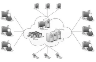
Cloud computing refers to the delivery of infrastructure components, software, storage and services over the Internet based on user demand with pay-as-you-go subscription. The architecture of cloud computing is given in the below figure:
Fig. 1 Cloud Computing Architecture
There are certain services and models working behind the scene making the cloud computing feasible and accessible to end users. The
working models for cloud computing are: Deployment
Models and Service Models. Deployment models
define the type of access to the cloud, i.e., how the cloud is located? Cloud can have any of the four types of access: Public, Private, Hybrid and Community.
Service Models are the reference models on which the
Cloud computing is based. These can be categorized into three basic service models as listed below:
Infrastructure as a Service (IaaS) is the delivery of technology infrastructure as an on demand scalable service. It provides access to fundamental resources such as physical machines, virtual machines, virtual storage, etc.
Platform as a Service (PaaS) provides the
runtime environment for applications,
development & deployment tools, etc.
Software as a Service (SaaS) model allows using software applications as a service to end users. SaaS is a software delivery methodology that provides licensed multi-tenant access to software and its functions remotely as a Web-based service.
The characteristics of cloud computing includes the following:
On-demand service
Flexibility
Elasticity
Scalability
Duplicability
Automation
Rapidity
The cloud environment has a
nondeterministic structure; hence it would cause a serious problem to perform tasks with a time limit. Therefore, prediction models are used to analyse the performance of the cloud to determine environment for users. The various prediction models are discussed in this survey.
II. LOADPREDICTION
When there is a dramatic change in load dynamically, it will cause frequent SLA violations. To avoid such violations, it is desirable to acquire the resources in earlier than the time when the load actually increases. Hence load prediction plays a crucial role.
resources with co-hosted applications cause fluctuations in the allocation.
III.PREDICTIONUSINGBAYESIANMODEL[1]
The fundamental idea of Mean Load
Prediction Based on Bayes Model [1] is to generate the
posterior probability from the prior probability
Distribution and the run-time evidence of the recent load fluctuations, according to Bayes Classifier. Bayesian classification consists of five main steps:
i. Determine the set of target states and the
evidence vector with mutually independent features
ii. Compute the prior probability distribution
for the target states based on the samples
iii. Compute the joint probability distribution for
each state
iv. Compute the posterior probability according
to the formula
v. Make the decision
based on the risk function
The metrics for evaluating prediction accuracy are Mean Squared Error (MSE)
and success rate. MSE between the
predicted load values and the true values calculated using the formula and it should be minimized.
Success rate is defined as the ratio of the number of accurate predictions to the total number of predictions. A prediction is deemed accurate if it falls within 10% of the real value. In general, the higher the success rate, the better, and the lower the MSE.
This Bayesian method outperforms other solutions by 5.6 – 50% in the long-term prediction.
IV. NEURALNETWORKBASEDLOAD PREDICTION
A neural network is a machine that is
designed to model the way in which the brain performs a particular task. For load prediction, neural network is used to predict the future load based on the past historical data.
A. Fast Up Slow Down (FUSD)2
In the FUSD method, the load forecasting is carried out using the equation:
E (t) = α * E(t – 1) + (1 – α) * O(t), 0 ≤ α ≤ 1,
Where E(t) is the estimated load and O(t) is the observed load during the time t.
This algorithm works properly if the prediction is in a very sequential order. To depict a more accurate forecasting the formula is changed to
E(t) = m * A(t – 1) where A is the actual load with respect to time and m is the multiplier.
m =
This also doesn’t forecast the actual future load to be allocated to the VM, it forecast a very close value nearer to the accurate.
B. K-ANFIS3
The Kalman filter and Adaptive Neuro-Fuzzy Inference system (K-ANFIS) algorithm first applies filtering process (Kalman filter) for the volatility characteristic of the load in cloud computing and then use ANFIS to forecast the load for the next phase.
The system is divided into three parts:
i.
The learning ability of the fuzzy rule setIF-THEN (Learning algorithm – BP algorithm and the least square estimation algorithm)
ii.
The membership function of the definitionof the data set
iii.
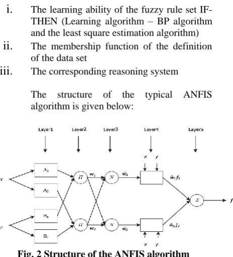
The corresponding reasoning systemThe structure of the typical ANFIS algorithm is given below:
Fig. 2 Structure of the ANFIS algorithm
In the ANFIS structure, the first layer is responsible for the ambiguity of the input signal. Here, the shape of the membership function changes with the change in parameters.
The second layer is responsible for the multiplication of the input signal, the output of each node represents the credibility of a rule.
The third layer is the i-node calculation. The
fourth layer and its summation (5th layer gives the
C. Kalman Smoothing weighted Support Vector Regression (KSwSVR)4
The KSwSVR prediction method is based on statistical learning technology, support vector regression (SVR), which is suitable for the complex and dynamic characteristics of the cloud computing environment. It integrates the SVR algorithm and the Kalman Smoothing technology.
The Kalman filter estimates the process state and then obtains feedback in the form of noisy measurements. The Kalman filter is used here since it estimates the hidden parameters indirectly from measured data and can integrate data from many measurements.
Support Vector Machines (SVM) method was proposed by Vapnik to solve the pattern recognition problems. SVM was promoted to SVR (Support Vector Regression) in 1998. SVR produces a decision boundary that can be expressed in terms of a few support vectors and can be used with kernel functions to create complex nonlinear decision boundaries. SVR is a very promising prediction model that outperforms the back propagation neural networks (BPNN) prediction algorithms.
The decision making process of KSwSVR method is given below:
Fig. 3 KSwSVR Decision Making Process
D. RVLBPNN5 Prediction Algorithm
BP Neural Network can effectively hide nonlinear relationships among the Cloud workloads. VLBP (Variable Learning rate Back propagation) enhances the convergence rate but slows down the update process of Mean Square Error (MSE). By incorporating variant concepts of a genetic algorithm with the BPNN, the new algorithm called the Rand Variable Learning rate BPNN (RVLBPNN) is implemented. This algorithm effectively adjusts the learning rate of the neurons in accordance with the trend of the MSE. The algorithm is explained in the following steps:
1) Generate a random number rand(u) (0 <
rand(u) < 1).
2) If rand (u) is less than a defined value (0.8),
then execute VLBP algorithm.
3) If rand(u) is greater than the defined value,
else if MSE has increased, then the learning rate is multiplied by a factor greater than 1; if MSE decreases after updating the connection weight, then the learning rate is multiplies by a factor between 0 and 1.
RVLBPNN algorithm can identify the global minimum point by effectively avoiding the local minimum points and hence improves the learning efficiency of the network neurons.
E. EEWMA5 (Enhanced Exponentially Weighted Moving Average) Prediction Algorithm
Two main ideas of this paper are:
Overload avoidance
Green computing
Overload avoidance: To reduce the number of
hotspots moves the VMs to the underutilized servers.
Green Computing: The underutilized servers
can be turned off. If the server is found to be underutilized, then the VMs of those servers can be moved to some other servers so that these servers can be made idle and they can be turned off.
To predict the resource needs of VMs in future, Average EWMA was used earlier. But EWMA is not suitable for the uprising needs. Hence the Enhanced EWMA prediction is used as follows:
E (t) = α * {(O(t – 1) + O(t)) / 2} + (1 – α) * O(t), α = 0.7
V. FEEDBACK BASEDLOADPREDICTION7
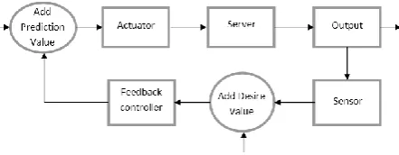
The feedback based prediction model is based on the difference between the predicted and the real value. It takes the system output into consideration. The block diagram of feedback prediction model is given below:
Fig. 4 Feedback Prediction Model
sensory data. It returns an error as feedback and involves itself in the future results. Sensors are often installed on actuators to search the environment and continuously correct the actions based on real data. The goals for the feedback based prediction model in the first test bed are:
1 – All tasks perform within the deadline
2 – The selected prediction model must be more effective than other models
3 – The prediction models must have better accuracy.
In the second test bed, efficiency is considered. 1 – To converge to the stable point during a reform process
2 – To reach the maximum user sharing 3 – To impose less cost for users
In the third test bed, prediction accuracy is observed.
VI. COMPARISONTABLEOFLOADPREDICTIONALGORITHMSINCLOUD
Load Prediction Methods in Cloud Parameters Merits Demerits
Host Load Prediction in a Google Compute Cloud with a Bayesian Model [1]
Mean Square Error (MSE) and Success rate
Outperforms other solutions by 5.6 – 50% in the long-term prediction.
Evaluated only using
Google’s cloud
Load Forecasting for Optimal
Resource Allocation in Cloud
Computing Using Neural Method [2]
Estimated load,
Actual load,
Observed load
-- Wastes a huge resource to
forecast
The Cloud Computing Load
Forecasting Algorithm Based on Kalman Filter and ANFIS [3]
Mean Absolute Error (MAE)
Better prediction accuracy --
Efficient Resources Provisioning
Based on Load Forecasting in Cloud [4]
Linear Prediction,
machine learning
technology – AR
Minimize prediction error,
improve resource
utilization, improves energy
saving, very stable
algorithm
Not integrated into an
automated cloud resource management system
RVLBPNN : A workload Forecasting Model for Smart Cloud Computing [5]
Mean Square Error
(MSE), local
minimum point
Facilitates better learning rate of neurons, Increases prediction accuracy
Periodicity effects of the workload behaviour can be incorporated to enhance the
prediction accuracy
.
Load Prediction Algorithm for
Dynamic Resource Allocation[6]
Estimated load,
Observed load
Overload avoidance, Green computing, works well on both increasing and
decreasing trend of
resources
--
A feedback based prediction model for real-time workload in a cloud [7]
Time series Helps the system to be
stable and amend itself. Automatic identification and resolution of anomalies.
Difficult to identify a
minimum requested resource that satisfies a time limit for a given workload.
VII.CONCLUSION
This paper summarizes the classification of load prediction methods and its impact on cloud environment. Efficient load prediction in cloud computing, leads to the betterment of cloud services. After prediction, various methods can be applied to minimize skewness so that the overall utilization of server resources can be improved.
REFERENCES
[1] Sheng Di, Derrick Kondo, Walfredo Cirne, “Host Load Prediction in a Google Compute Cloud with a Bayesian Model”, SC '12: Proceedings of the International Conference on High Performance Computing, Networking, Storage and Analysis, 10-16 Nov. 2012
[3] Jian Sun and Yi Zhuang, “The Cloud Computing Load Forecasting Algorithm Based on Kalman Filter and ANFIS”, 4th International Conference on Machinery,
Materials and Computing Technology (ICMMCT 2016) [4] J Rongdong Hu, Jingfei Jiang, Guangming Liu, and Lixin
Wang, “Efficient Resources Provisioning Based on Load Forecasting in Cloud”, The Scientific World Journal, Hindawi Publishing Corporation, Vol 2014, Article ID 321231.
[5] Yao Lu, John Panneerselvam, Lu Liu and Yan Wu, “RVLBPNN: A workload Forecasting Model for Smart Cloud Computing”, Scientific Programming, Hindawi Publishing Corporation, Vol 2016, Article ID 5635673. [6] M.Lavanya and V.Vaithiyanathan, “Load Prediction
Algorithm for Dynamic Resource Allocation”, IJST, Vol 8(35), December, 2015, ISSN (Print): 0974 - 6846. [7] Babak Esmaeilpour Ghouchani, Azizol Abdullah, Nor
Asila Wati Abdul Hamid, Amir Rizaan Abdul Rahman, “A feedback based prediction model for real-time workload in a cloud”, Journal of Theoretical and Applied Information Technology, Vol 87. No.3, 31st May 2016, ISSN (Print):