Shock-induced noise in 2D sub- and supersonic mixing layers

Eric Canc`es & Jean-Fr´ed´eric Gerbeau, Editors DOI: 10.1051/proc:2007009

SHOCK-INDUCED NOISE IN 2D SUB- AND SUPERSONIC MIXING LAYERS

J. Schulze

, Ch. Schaupp

, J. Sesterhenn

, R. Friedrich

, J. Berland

, Ch.

Bogey

and D. Juv´

e

Abstract. A numerical code solving acoustic analogies to predict shock-induced noise is developed. Both Lighthill’s analogy and the one of Ffowcs-Williams and Hawkings (FWH) are implemented and compared to the acoustic far field of the direct numerical simulation (DNS) in detail. In addition to this the linearized Euler Equations (LEE) are used to propagate into the acoustic far field and the results are also compared to the DNS-data. With a two dimensional mixing layer in a subsonic test case and a Reynolds number based on the initial shear layer thicknessRe_δω0 of 1.42·105, a first application of the code is performed. To investigate the shock-induced noise, a two dimensional supersonic mixing layer with an impinging oblique shock is simulated. The results of the analogies for the shock-induced noise are in good agreement with the acoustic far field of the DNS. The accuracy of the FWH-method is better than the one of Lighthill’s analogy.

1.

Introduction

Understanding and predicting the sound generation processes by supersonic turbulent jets issuing for example from the exhaust of civil and military aircraft is an issue of great interest: Reduction of noise, polluting the environment is desired and minimization of damage to engine or nozzle parts due to high-intensity sound radiated by the jet flow is necessary.

The supersonic jets considered here are either over- or underexpanded. Thus, a shock-cell structure exists within the jet core, which gives rise to additional noise components, to be investigated here: Shock–associated noise and jet screech.

Different approaches to numerical simulation of noise generation within these jet flows have been adopted by the participants of this research project, conducted within the framework of CEMRACS 2005. While the French group from ´Ecole Centrale de Lyon focused on Large-eddy simulation of a planar, supersonic jet subject to the screech phenomenon, the German participants from Technische Universit¨at M¨unchen performed DNS of the isolated planar mixing layer–compression wave interaction.

In this way, it was possible on the one hand to capture the complete near acoustic field including mix-ing noise, shock-associated noise and jet screech, and to demonstrate the capabilities of the LES method to handle problems of this kind. On the other hand, the sound generation by interaction of turbulence with the oblique compression/expansion structures, which is of fundamental importance within the phenomena of shock-associated noise and jet screech, could be investigated in detail.

The CEMRACS 2005 event with a focus on computational aeroacoustics offered an excellent opportunity to define and perform joint work related to the supersonic jet noise problem. Propagation of sound computed by

1_{Technische Universit¨at M¨unchen, Germany} 2_{Ecole Centrale de Lyon, France}´

c

EDP Sciences, SMAI 2007

DNS/LES close to the jet or the mixing layer, respectively, into the far acoustic field was selected as focus of our work during CEMRACS 2005. Different approaches to far field sound propagation have been applied to the oblique shock/shear layer interaction case; the methods used (propagation by Lighthill’s analogy, Ffowcs-Williams and Hawkings analogy and linearized Euler equations) and the results obtained shall be presented in the following.

2.

Governing theory

In this section, Lighthill’s analogy and the FWH-method are presented. For both analogies the numerical procedure is explained in detail. The used LEE-method is described at the end of this chapter.

2.1.

Lighthill’s Analogy

Lighthill’s [24] 1951 idea was to make a rearrangement of the compressible and unsteady Navier-Stokes (NS) equations into an inhomogeneous wave equation without any approximations or modeling. The right hand side of the new found wave equation can now be interpreted as acoustic source term called Lighthill’s source:

∂2_ρ ∂t2 −c

2 0Δρ =

∂2_Tij ∂xi∂xj

(2.1)

wherec0 is the ambient speed of sound andTij is Lighthill’s stress tensor defined as:

Tij =ρuiuj+ (p−ρc2₀)δij−τij; (2.2)

primed variables denote fluctuations likep=p−p0. Far away from the turbulent aerodynamic field the tensor Tij disappears and can be set to zero. So the sources only play a role in a limited volume including the turbulent fluctuations. As estimated by Goldstein [20] and Lighthill [24] the dominant part of the sources are the Reynolds stressesρuiuj. Unlike most articles in the literature, where the other two parts of the tensorTij are neglected, we will use the complete source, since the deviation of the isentropic behavior (p−ρc2

0)δij plays a role for supersonic cases.

2.1.1. Numerical algorithm

The solution of Lighthill’s equation is obtained using the three dimensional free space Green’s function. It can be written for space derivatives of Lighthill’s stress tensor in the following form:

p_{(x, t) =} 1 4π

V 1

r ∂2_T

ij

∂yi∂yj

y, t−_cr

0

dy. (2.3)

where r = |x−y| is the distance between the observer’s location y and the the source x. V is the volume including all relevant acoustic sources. These sources have to be evaluated at the retarded timeτ =t− r

c0 which makes interpolation between stored time steps necessary. This method was also used in [6] and differs from the method used in [34], where a Green’s function in frequency space is used to avoid interpolation in time.

0 0.2 0.4 0.6 0.8 1 1.2

0% 20% 40% 60% 80% 100%

Figure 1. Implemented window function; Example: inlet: 33%, outlet: 10%

Low-pass filtering.If the temporal resolution of the sources is too small (due to storage used), a low-pass filtering of Lighthill’s sources can avoid high frequency noise in the far field. In the present study a Butterworth low-pass filter was used to adjust temporal badly resolved sources. It has to be mentioned that the filtering of the source only reduces the high frequency noise but is not effecting a better solution.

Integration. Subsequent to the interpolation, the sources are integrated over the source volume V. The integration is approximated with the midpoint rule, which is a simple but fast method. An application of a method with a higher resolution, like the Simpson rule, is by reason of the later explained ”QuickSort”-method not such straightforward.

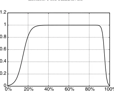
Window function. Most technical applications make it impossible to locate all sources in a closed volume; e.g. in a jet a convective flow transports the sources through a fixed volume. It is therefore essential to add special inflow and outflow conditions to the near field. Otherwise noise from the region of the in- and outlet would cover the far field. In the present study, a window function fades the sources slowly in the near field and out on the outlet. It consists of two hyperbolic tangent functions and can be defined by:

f(x) = 1 2

tanh

2(x−xstart−b v 2 ) 1 bv (2.4) −tanh

2(x−xend+b h 2 ) 1 bh

where the parameters bi, i =v, h modify the width of the window in- and outlet. These parameters have to be adjusted carefully for each case. It could be shown that the width of the window in- and outlet has to be at least as large as the distance of two convecting acoustic sources (e.g. vortices). In fig. 1 an example of a possible window function is presented.

Averaging.As described for example in Bogey et al. [6], it is necessary to calculate and subtract the average of the sources in order to obtain a centered pressure fluctuation. The new found source term is obtained by:

∂2_T

ij

∂xi∂xj ∗

= ∂

2_T

ij

∂xi∂xj −

∂2_Tij ∂xi∂xj.

(2.5)

The temporal average is thereby calculated over the sum of all stored time steps divided by their number:

∂2T_ij ∂xi∂xj ≈

N

z=1 ∂2_Tij ∂xi∂xj|

z/N, (2.6)

Figure 2. Schematic view of the flow situation in the far field with a moving medium (velocityu).

aircraft, propelled by the jet engine). For this case the free space Green’s function has to be adjusted to take the mean-flow effects into account. If the medium in the acoustic far field is not at rest the velocity of propagation of the acoustic waves is no more uniform in all directions, but a vectorial sum of all concerned velocities. An observer in an upstream direction of a source would hear their signal later than an observer in flow direction. According to this a mean-flow in the far field also affects the retarded time (τ =τ(c)).

The problem can be formulated in vectorial notation:

c0Δt+uΔt−r=0, (2.7)

where Δtdenotes the runtime of a signal from the sourcexto the far fieldywith the virtual observer location

y _{(see fig. 2).}

In order to reduce the problem, the following simplifications are used:

• u= (u1,0,0)T; parallel mean-flow

• r= (r1, r2,0)T; two-dimensional problem

The new found retarded timeτ∗=t−Δtcan now be determined to:

τ∗_=t− 1

c0(Ms2−1)

MsΔx− Ms2Δx2+r2

, (2.8)

with the Mach number Ms of the parallel flow in the far field and Δx = x1−y1. Equation (2.8) has to be

inserted in a modified Green’s function:

p_{(x, t) =} 1 4π|1 +MsΔ_rx|

V 1

r ∂2_Tij ∂yi∂yj

(y, τ∗) dy. (2.9)

Numerical issues.The solution of Lighthill’s analogy with Green’s function needs the information of the acoustic sources stored over a certain period of time in order to evaluate the sound in a far field with a certain size. To calculate the acoustic fluctuation at one point in the far field, all this point’s affecting sources have to be taken into account. The calculation of more than one point (a field) makes it necessary to read each saved time step more than once which is temporal expensive. In the present code all existing retarded times (nret.times=nnearfield·nfarfield∼109, for an average 2D problem) are sorted by their length to recognize which

2.2.

Ffowcs-Williams and Hawkings Analogy

Most of the above mentioned numerical issues are not necessary for the Ffowcs-Williams and Hawkings method. The FWH-equation is based on Lighthill’s analogy and represents an advanced Lighthill-equation. Again, the FWH-equation is a rearrangement of the compressible NS-equations and includes a source term on their right hand side. Unlike Lighthill’s method, the sources are not stored in a closed volume with all the turbulent fluctuations but on a surface surrounding all acoustic sources and, in addition to this, in the area outside this surface (Tij). In most cases, the FWH-equation is applied to problems with moved bodies like the sound radiation of a rotor blade. For this case the sources have to be taken into account on the surface of the rotor blade and in the surrounding medium (vortices caused by the rotor blade). It is needles to say that the sources surrounded by the surface - in our case the sourcesin the rotor blade - have to be set to zero. If one tries to predict the radiated sound of a free jet, no solid surfaces are present. The surface, on which a part of the FWH-sources are stored, can now be chosen arbitrary. It is however useful to choose a surface which surrounds all the turbulent fluctuations because all the sourcesTij are zero outside the volume and, as aforementioned, have to be zero in the volume, also. In this case, only sources on a surface remain and the volume integration in Lighthill’s analogy turns into a surface integration for the FWH-equation which reduces the computational costs drastically. It has to be mentioned that these FWH-sources are based on acoustic fluctuations in the acoustic far field and not on noise generating turbulent fluctuations in the near field as they are the basis for Lighthill’s analogy.

The FWH-equation in integral notation, for a free jet with no solid surfaces, is obtained by:

4π{p(x, t)·H(f)}= ∂

∂t

S

_ρui

r ni

τdS

−_∂x∂

i

S

ρuiuj+Pij

r nj

τ

dS, (2.10)

withPij =pδij−τij and the Heaviside-functionH(f) which is zero in the area surrounded by the the surface

S. The indexτ indicates that the sources have to be evaluated at the retarded time, whereas the retarded time can be calculated by eq. (2.8) to take mean flow effects into account. In comparison to Lighthill’s analogy the FWH-sources are not a scalar but a symmetric matrix which increases the amount of storage about the sixfold. This source-matrix is multiplied by the normal vectorni of the surface and then interpolated at the retarded time. The interpolation scheme can be adopted from the Lighthill analogy whereas the integration has to be reduced to a surface integration. All other numerical issues, like the window-function or the averaging and filtering of the sources, are unnecessary for the FWH-method.

2.3.

Far-field sound propagation using LEE

A hybrid zonal approach can be implemented to predict the far-field noise. In this approach, the near-field data provided by the DNS computation is extrapolated using a simplified set of equations, allowing long-range propagation of acoustic waves.

In the present work, the two-dimensional linearized Euler Equations (LEE) are solved beyond an extrapolation line, which is specified by the DNS near-field. Assuming that time-dependent perturbations are small, and keeping only the first order terms in the Euler equations yields the LEE, given in two dimensions by,

∂U ∂t +

∂E ∂x +

∂F

where,

U = [ρ, ρ₀u, ρ₀v, p] (2.12)

E = [ρu0+ρ0u, ρ0u0u+p, ρ0u0v, u0p+γp0u] (2.13) F = [ρv0+ρ0v, ρ0v0u, ρ0v0v+p, v0p+γp0v] (2.14)

The termH, defined as,

H= [0,(ρ0u+ρu0)· ∇u0,(ρ0u+ρu0)· ∇v0,(γ−1)p∇ ·u−(γ−1)u· ∇p0] (2.15)

takes into account the mean flow inhomogeneities, withu= (u, v) andu₀= (u0, v0). The specific heat ratio γis equal to 1.4.

The LEE are solved using the low dispersive and low dissipative explicit numerical algorithms developed by Bogey & Bailly [9]: optimized eleven-point finite differences are implemented to compute spatial derivatives, and selective filtering is performed with optimized eleven-point filter. Time integration is carried out by an optimized fourth-order six-stage low-storage Runge-Kutta scheme [4]. The non-reflecting boundary conditions of Tam & Dong [43] are implemented to model a free-field space. More details on the extrapolation procedure are provided in [5], where LEE are used to propagate screech tones predicted by LES into the far-field.

3.

Application

In this chapter, numerical results of theLighthill/FWH-code and theLEE-code for two application cases are presented. These are:

(1) Subsonic mixing layer (both velocities subsonic); computed with Lighthill’s analogy (two-dimensional computation).

(2) Supersonic mixing layer interacting with an oblique shock; computed with Lighthill’s analogy, the FWH method and LEE-propagation (two-dimensional computation).

To save computational time, the used DNS cases are simulated in a two-dimensional domain. It has to be mentioned that in these idealized two-dimensional computations the acoustic source diverges from a real three-dimensional case. As a consequence, effects like the roll up and pairing of vortices might be stronger and lead to a raised acoustic noise level. For a detailed description of the used DNS cases see [37].

3.1.

Subsonic mixing layer

The subsonic mixing layer is forced with its most unstable frequencyf₀and its first sub-harmonic, in order to achieve a vortex pairing at a more or less fixed location. This vortex pairing is the dominant acoustic source in this test case and emits an acoustic signal with the frequency of the vortex pairing (fP =f0/2). Michalke [28]

showed with a linear stability analysis that this frequency can be determined to:

f0= 0.132u

c

δ0

ω

, (3.16)

with the common velocityuc = (u1+u2)/2 and the initial mixing layer thickness δω0. The parameters of the DNS for this test case are listed in tab. 1.

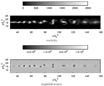
A result of the DNS (near field) for the vorticity and the divergence of Lighthill’s stress tensor (acoustic source) is shown in fig. 3, where thex-location of the vortex pairing seems to be aroundx= 90·δω0. This point is the origin of the dominant acoustic source. In fig. 4 theLighthill-solution for this first test case is presented. For this calculation, mean-flow interactions (eq. (2.8)) are taken into account.

Case _I

u1 0.4c0 Lx/δω0 346

u2 0.2c0 Ly/δ0ω 157

μ0 1.824·10−5mkg_·s (Air) nx 512

Reδ0_ω 1.42·105 ny 384

Table 1. Parameter of the DNS for the subsonic mixing layer (test case one)

vorticity

Lighthill-source

Figure 3. Subsonic mixing layer;top: vorticity;bottom: divergence of Lighthill’s stress tensor

the emitted sound but also the noise is visible more detailed (including the filtered case; see the following paragraph).

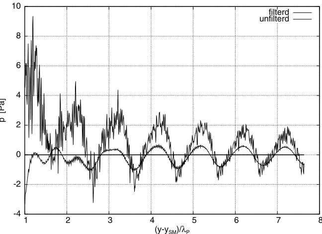
In order to reduce the noise in the far field, the Lighthill sources are filtered in time with a low-pass Butter-worth filter at a cutoff-frequency offcut= 2.5fP = 5.0f0. Through the application of the filtering, the noise in

the far field of theLighthill-solution could be reduced but also the amplitude of the acoustic waves is reduced. In fig. 5 a cut through the far field is shown for both the filtered and the unfiltered case.

The influence of the parameters of the window function is demonstrated in fig. 6, with a series of snapshots of a small part of the far field. Modified is the width of the window function at the inlet, while the width of the outlet is kept constant at 26δω0. To reduce the noise from the inlet such that it is negligible in comparison to the expected dominant acoustic field, the width of the window-inlet has to be at least 10.5·δ0ω which is about the distanceδs0of two vortices, entering the near field. This result emanates from fig. 7, where the relative error of the different far fields, based on a far field with a wide window-inlet, is plotted over the window-width bv.

Figure 4. Acoustic far field; computed with Lighthill’s analogy, pressure fluctuation±5 [Pa],

WENO-4. The top left-hand corner of the figure is physically incorrect because of missing time steps in the past of the mixing layer.

pairing is not visible. However, the Lighthill-solution is predicting the dominant acoustic noise source of the vortex pairing with the expected frequency. In the following test case a comparison between the DNS and the analogies is presented.

3.2.

Supersonic mixing layer with shock

In this test case shock-induced noise is investigated. This is achieved by a turbulent sub-/supersonic mixing layer with an impinging oblique shock. In contrast to the above discussed subsonic case, the mixing layer of this test case is only forced by its most unstable frequencyf0to avoid a vortex pairing. As we will see, a vortex

pairing occurs downstream of the interaction point between shock tip and mixing layer, anyway. Although this pairing emits a louder acoustic wave than the shock interaction, it won’t disturb us because shock-induced noise is emitted mainly in the upstream direction and the noise of the supersonic vortex pairing in the downstream direction (see fig. 8 (left) for details). In fig. 8 (right) the full Lighthill source including the acoustic far field of the DNS is visualized. The shock-induced noise is clearly visible in the upstream direction.

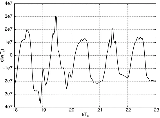
For the interpolation of the source at the retarded time their temporal evolution is important. The source is stored with a temporal resolution of Δt= 1/(16·f0). This seems to be a sufficient condition to satisfy the

Nyquist-criterion and to guarantee a physical correct reconstruction of the source (see also fig. 9).

-4 -2 0 2 4 6 8 10

1 2 3 4 5 6 7 8

p’ [Pa]

(y-ySM)/λP

filterd unfilterd

Figure 5. Cut through the far field iny-direction atx= 100δ_ω0 divided by the wavelengthλ_P

and measured from the middle of the mixing layerySM; filtered and unfiltered case.

0δ0

ω 2.6δω0 6.5δω0 13δω0

Figure 6. Far field for different parameters of the window function. Modified is the width of

the window function at the inlet, while the width of the outlet is kept constant at 20%. Same color scaling for all cases (±5.0 [Pa])

Case _II

u1 1.44·c0 Lx/δ0ω 346

u2 0.216·c0 Ly/δω0 85

μ0 8.365·10−3mkg_·s nx 512

Reδ_ω0 1.90·103 ny 384

Table 2. Parameters of the DNS for the mixing layer with shock.

calculating the total pressure and the analogies only the pressure fluctuation. So the ambient pressurep0 has

to be subtracted from the DNS data.

0.001 0.01 0.1 1 10

0 0.2 0.4 0.6 0.8 1 1.2 1.4 1.6 1.8 2

rel. error

b/δs 0

Figure 7. _{Relative error of different far fields (fig. 6), based on a far field with a wide}

window-inlet, plotted over the window width bv divided by the distanceδ0s of two entering dominant acoustic sources (vortices)

Figure 8. Left: Instantaneous dilatation field for the mixing layer with shock (DNS); color

scale±100 [1/s];Right: Instantaneous field of the full Lighthill source for the same case (DNS); color scale±5·106_[kg/(s2_m3_)]

qualitative differences to the DNS can be seen in this visualization. Both amplitude and position of the two calculations are in good accordance to each other. In a cut through the far field the differences can be seen more detailed (fig. 12). A high frequency noise superposes the far field of theLighthill-solution and is most dominant in the near of the mixing layer (y/δ0

ω<40).

-4e7 -3e7 -2e7 -1e7 0 1e7 2e7 3e7 4e7

18 19 20 21 22 23

div(T

ij

)

t/T0

Figure 9. Temporal evolution of the full Lighthill source ( ∂

2_T

ij

∂xi∂xj) measured at the interaction

point of shock tip and mixing layer over five periodsT₀

the acoustic relevant sources. This refraction effect is particularly dominant in the case of the sub-/supersonic mixing layer with shock. Lighthill’s analogy, with the use of a Green’s function, is not taking these effects into account, since the speed of sound is expected to be constant in the whole computational domain (see eq. (2.3)). Similar to the method used for the derivation of eq. (2.9), the information of the local speed of the acoustic signal should be included in such an analysis (like a modified retarded time). These effects are negligible for the FWH and the LEE method since the used sources are already in the acoustic far field where a constant speed of the acoustic wave propagation can be assumed (except for the effects of a parallel meanflow, see eq. (2.9)).

The solution for the FWH-method is presented in fig. 11 (bottom right). It includes the acoustic pressure fluctuation in the far field and a part of the source (_∂t∂(ρv), DNS) in the near field. For this two dimensional case, the surface integration turns into a one dimensional problem, so the sources have to be stored only on a line (red line in the near field of fig. 11). This ”source-line” has to be placed on an appropriate location in the near field, which should be in general far away from any aerodynamic perturbations. To specify this place more precisely, a parameter study with a varying position of the source-line iny-direction has been performed. The resulting far fields of each different source-line are then compared to the far field of the source-line with the largest distance to the mixing layer and their relative error is identified. In addition to this we use the Q-criterion of Hunt et al. [22], which defines the zones where rotation is predominant, to measure the strength of the aerodynamic perturbations:

Q= 1

2[rijrij−sijsij], (3.17)

with the strain rate tensorsij and the rotation tensorrij. In fig. 10 both the L2-norm of the Q-criterion and

the above mentioned relative error are plotted with a logarithmic scaling (to compare both curves an arbitrary scaling is used). It can be shown that the Q-criterion is linked to the relative error and therefore acts as an indicating value for the positioning of the source-line. In our case the source-line is well placed in a distance to the mixing layer of at least 20δ0ω. In addition to this we can see that the position of the FWH-surface (”source-line”) is not sensitive, since the relative error is constant once we are in the acoustic far field.

0 1 2 3 4 5 6 7 8 9

0 10 20 30 40 50 60 70

y/δω0

~log(rel. error) ~log(||Q-criterion||)

Figure 10. _{Comparison of the Q-criterion (}L_{2-norm) and the relative error between the far}

fields for different positions of the stored sources. Center of the mixing layer aty= 0δ0ω

The results of the linearized Euler Equations are presented in fig. 11 (bottom left) and, in a comparison to the DNS and the analogies, in fig. 12. The results seem to match with the ones of the DNS.

4.

Concluding remarks

TheLighthill/FWH-code is implemented to evaluate the sound emitted by the Lighthill/FWH-sources with an integral formulation. Different numerical schemes for the treatment of the source are tested to determine their influence to the numerical solution, like the influence of the window function, the filtering and averaging of the source and different interpolation procedures. In addition to this, we compared the the results to the LEE propagation.

A two-dimensional subsonic mixing layer was used as a first application case for the Lighthill-sources. Al-though we observed a superposition of spurious high frequency noise in the far field of the Lighthill solution, the dominant frequency of the vortex pairing could be identified. The expected sound in the DNS was not clearly visible in this ”small” computational domain, so no direct comparison to the DNS was possible. In order to minimize high frequency noise in the far field, low pass filtering of the sources was necessary.

second test case was used to investigate shock-induced noise with the Lighthill- and the FWH-method and also the LEE. It could be shown that the accordance between the FWH-method and the DNS was much better than the one of Lighthill’s solution. Close to the near field the differences between the DNS and Lighthill’s analogy were most dominant. Far away from the aerodynamic fluctuations, the position and the frequency of the acoustic waves in Lighthill’s analogy match with the ones of the DNS, although the amplitude differs. Again, high frequency noise superposed the solution of both analogies. With a parameter study, theL2-norm

of the Q-criterion was found to be an indicating value for an appropriate position of the source-surface in the FWH-method. This value seems to be an important parameter to optimize the hybrid simulation.

DNS Lighthill

LEE FWH

Figure 11. Comparison of all used numerical prediction methods. Top left: DNS, (p[±600

Pa]) (for a more descriptive visualization, the area around the mixing layer has a different color scaling (p[±12000 Pa]). Top right: Lighthill solution, (p[±600 Pa]), including the source-area in the near field (_∂x∂2Tij

i∂x_j). Bottom left: LEE propagation, (p[±600 Pa]), far field starts at y/δ0

ω ≈ 50, the near field shows a part of the FWH-source ( ∂

∂t(ρv)) [±3·103]. The red line denotes the location of the variables, used as input data for the LEE-code. Bottom right: FWH-solution, far field starts aty/δ0ω≈50, near field shows a part of the FWH-source (

∂ ∂t(ρv)) [±3·103]. The red line denotes the location of the sources, used as input data for the FWH-code.

in relation to Lighthill’s analogy, is that a modification of the sources like windowing, filtering or averaging is needless. The results of the LEE reproduce the overall shape of the near acoustic field provided by the DNS. In comparison to the analogies, no high frequency noise is visible in the solution of the LEE-propagation.

-4000 -3000 -2000 -1000 0 1000 2000

30 40 50 60 70 80 90 100 110

p’ [Pa]

y/δ_ω0

FWH LIGHTHILL DNS LEE

Figure 12. Comparison of the analogies (Lighthill/FWH) and the LEE-propagation to the

DNS, Pressure-fluctuation.

References

[1] Andersson, N., Erikson, L., Davidson L. (2004). A Study of Mach 0,75 Jets and Their Radiated Sound Using Large-Eddy Simulation.10th AIAA/CEAS Aeroacoustics Conference (2004)

[2] Bailly, C. and Juv´e, D. (2000). Numerical solution of acoustic propagation problems using linearized Euler equations.AIAA J. 38(1):22-29

[3] Bailly, C., Bogey, C. (2004). Contributions of computational aeroacoustics to jet noise research and prediction. Int. J. of Comp. Fluid Dynamics 18(6):481-491

[4] Berland J., Bogey C. and Bailly C., (2006). Low-dissipation and low-dispersion fourth-order Runge-Kutta algorithm.Comput. Fluids.

[5] Berland J., Bogey C. and Bailly C., (2006). Large eddy simulation of screech tone generation in a planar underexpanded jet. 12th AIAA/CEAS Aeroacoustics Conference, 8-10 May, Cambridge, Massachusetts, USA. AIAA Paper 2006-2496.

[6] Bogey, C. Bailly, C. and Juv`e, D. (2000). Numerical simulation of sound generated by vortex pairing in a mixing layer.AIAA Journal 38(12):2210-2218

[7] Bogey, C. Bailly, C. and Juv`e, D. (2001). Noise computation using Lighthill’s equation with inclusion of mean flow - acoustic interaction.AIAA Paper 2001-2255

[8] Bogey, C., Gloerfelt, X. and Bailly, C. (2003). Illustration of the inclusion of sound-flow interactions in Lighthill’s equation. AIAA J. 41(8):1604-1606

[9] Bogey C. and Bailly C. (2004). A family of low dispersive and low dissipative explicit scheme for flow and noise computations. J. of Computational Physics 194:194-214.

[10] Colonius, T., Lele, S. and Moin, P. (1997). Sound generation in a mixing layer.J. of Fluid Mech. 300:575-409

[11] Colonius, T., Mohseni, K., Freund, J., Lele, S. and Moin, P. (1998). Evaluation of noise radiation mechanisms in a turbulent jet.Center for Turbulence Research 1998

[12] Crighton, D. G. (1975). Basic principles of aerodynamic noise generation.Prog. Aerospace Sci., 16(1):31-96

[13] Hardin, J. C. and Hussaini, M. Y. (1993). Computational aeroacoustics for low Mach number flows.Computational Aeroa-coustics, Springer Verlag (1993) S. 50-68

[15] Ehrenfried, K. (2003). Str¨omungsakustik II.Vorlesungsskript. Technische Universit¨at Berlin.

[16] Farrasat, F., Doty, M. and Hunter, C. (2004). The acoustic analogy - a powerfull tool in aeroacoustics with emphasis on jet noise prediction.10th AIAA/CEAS Aeroacoustics Conference , Manchester, United Kingdom, May 10-12, 2004

[17] Farrasat, F. and Posey, J. W. (2003). The role of analytic methods in computational aeroacoustics.International Journal of Aeroacoustics 1(3):207-240

[18] Friedrich, R. (2002). Kompressible Str¨omungen mit Reibung und W¨armeleitung.Fachgebiet Str¨omungsmechanik. Technische Universit¨at M¨unchen.

[19] Garc´ıa, A. (2004). Weighted ENO y aplicationes.Departamento de Mathem´atica Aplicada. Universitat de Val´encia (Spain) [20] Goldstein, M. E. (1976). Aeroacoustics.McGraw-Hill, New York, 1976

[21] Hoare, C. A. R. (1962). QuickSort.Computer Journal 5(1):10-15

[22] Hunt, J. C. R., Wray, A. and Moin, P. (1988). Eddies, stream, and convergence zones in turbulent flows.Center for Turbulence Research Report CTR-S88

[23] Juv´e, D. (2004). Two topics in computational aeroacoustics.DFG-CNRS Seminar, Orl´eans, september 6-7, 2004

[24] Lighthill, M. J. (1952). On sound generated aerodynamically-I. General theory.Proceedings of the Royal Society of London 221(A 1107):564-587

[25] Lilley, G. (1974). On the noise from jets.AGARD CP-131 pp. 13.1-13.12

[26] Liu, X., Osher, S. and Chan, T. (1994). Weighted Essentially Non-oscillatory Schemes.J. of Computational Physics 115:200-212

[27] Manning, T. (1999). A numerical investigation of sound generation in supersonic jet screech. PhD thesis. Department of aeronautics and astronautics. Stanford University

[28] Michalke, A. (1964). On the inviscid instability of the hyperbolic-tangent velocity profile.J. of Fluid Mech. 19:543-556 [29] Mitchelle, B., Lele, S. and Moin, P. (1999). Direct computation of the sound generated by vortex pairing in an axisymmetric

jet.J. of Fluid Mech. 383:113-142

[30] Morris, J, Farassat, F. (2002). Acoustic analogy and alternative theories for jet noise prediction.AIAA J. 40(4):671-680 [31] Powell, A. (1953). On the mechanism of choked jet noise.Proceedings of the Royal Society of London B, 66:1039-1056 [32] Powell, A. (1953). On the noise emanating from a two-dimensional jet above the critical pressure. Aeronautical Quaterly,

4(2):103-122

[33] Powell, A. (1954). The reduction of choked jet noise.Proceedings of the Royal Society of London B, 67(4):313-327

[34] Rembold, B., Freund, J. and Wang M. (2002). An evaluation of LES for jet noise prediction.Center for Turbulence Research. Proceedings of the Summer Program 2002.

[35] Rembold, B. (2003). Direct and large-eddy simulation of compressible rectangular jet flow.PhD thesis. Swiss Federal Institute od Technology Zrich.

[36] Rienstra, S. and Hirschberg, A. (2002). An introduction to acoustics.Eindhoven University of Technology.

[37] Schaupp, C. (2004). Numerische Untersuchung stossinduzierten L¨arms.Diplomarbeit, Fachgebiet Str¨omungsmechanik, Tech-nische Universit¨at M¨unchen, 2004

[38] Sebastian, K., Shu, C. (2003). Multidomain WENO finite difference method with interpolation at subdomain interfaces. Journal of Scientific Computing 19,Nos 1-3

[39] Sesterhenn, J. (2001). A characteristic-type formulation of the Navier-Stokes equations for high order upwind schemes.CAF 30(1):37-67

[40] Shu, C. 2003. High-order finite difference and finite volume WENO schemes and discontinous Galerkin methods for CFD. Int. J. of Comp. Fluid Dynamics 17(2):107-118

[41] Tam, C. K. W., Ahuja, K. K., Jones, R. R. (1994). Screech tones from free and ducted supersonic jets.AIAA J., 31(5):917-922 [42] Tam, C. K. W.(1995). Computational aeroacoustics: Issues and methods.AIAA J. 33(10):1788-1796

[43] Tam C.K.W. and Dong Z. (1996). Radiation and outflow boundary conditions for direct computation of acoustic and flow disturbances in a nonuniform mean flow.J. of Computational Acoustics 4(2):175-201.

[44] Numerical simulation of flow-induced noise by means of the hybrid method with LES and aeroacoustic analogy.Dissertation. Fachbereich Maschinentechnik der Universitt Siegen.