Design a Guidance Law Considering Approximation of Missile Control Loop Dynamics Using Adaptive Back-Stepping Theory

(1)

Iranian Journal of Electrical & Electronic Engineering, Vol. 14, No. 3, September 2018 204

Design a Guidance Law Considering Approximation of Missile

Control Loop Dynamics Using Adaptive Back-Stepping

Theory

V. Behnamgol*(C.A.)_{, A. R. Vali* and A. Mohammadi*}

Abstract: In this paper, a new guidance law is designed to improve the performance of a homing missiles guidance system in terminal phase. For this purpose first of all, the two dimensions equations of motion are formulated, then the approximation dynamic of missile control loop is added to these equations which are nonlinear whit unmatched uncertainty. Then, a new adaptive back-stepping method is developed in order to control this system. An adaptive term is used in the control law that is converged to the uncertainty. This convergence is proved based on Lyapunov stability theorem. Therefore using this adaptive term in the control law can be eliminated the uncertainty. Based on this algorithm, a new guidance law is designed. Then its performance is compared with common guidance laws in a guidance loop simulation in the presence of control loop dynamics.

Keywords: Guidance Law, Control Loop Dynamics, Adaptive Back-Stepping Control, Unmatched Uncertainty.

1 Introduction1

oming missiles guidance system consists of two guidance and missile control loops. The outer is guidance loop and the inner is missile control loop. In the guidance loop, the proper guidance commands are produced to modify the missile trajectory and reach it to the target. The guidance commands (missile lateral acceleration) are generated by guidance law

.

The guidance law is designed by using mathematical rules or control theories considering relative kinematics between the missile and the target

.

The guidance commands are implemented by the missile control loop [1-4]

.

So it can be said that the missile control loop acts as an actuator in the homing missiles guidance loop

.

In tactical missiles, the proportional navigation (PN) family are widely applicable laws implemented in

Iranian Journal of Electrical & Electronic Engineering, 2018. Paper first received 25 March 2017 and accepted 28 February 2018. * The authors are with the Department of Control Engineering, Malek Ashtar University of Technology, Tehran, Iran.

E-mails: vahid_behnamgol@mut.ac.ir, ar.vali@aut.ac.ir and

ali_mohammadi@yahoo.com. Corresponding Author: V. Behnamgol.

terminal phase of many missiles

.

This guidance law is based on nullifying the line of sight (LOS) rate

.

To intercept maneuvering targets, the augmented proportional navigation (APN) is proposed which needs the target maneuvers measurement or estimation. Therefore it leads to a significant increase in cost and of course complicated calculations [1-4]. PN family is designed based on mathematical theories

.

In recent years, the guidance law is considered as guidance loop controller and designed using control theories. From this point of view, the relative kinematic between missile and target is a process must be controlled. The outputs of this process are some variables such as LOS rate and closing velocity. These variables are measured by seeker and are sent to the guidance section to generate guidance commands.

Regarding the nonlinear kinematic relations in the terminal phase, nonlinear control theories and in especial case Lyapunov stability theory have been used to design the guidance law [5,6]. In the presence of uncertainties such as target maneuvers, sliding mode control theory has been used to design nonlinear and robust guidance laws

.

In this case, the guidance law only used the target maneuvers bound. Hence target maneuvers measurement or estimation is not required

.

H

(2)

Iranian Journal of Electrical & Electronic Engineering, Vol. 14, No. 3, September 2018 205 LOS rate is commonly used to introduce sliding

variables in sliding mode guidance laws

.

Then, missile acceleration has been designed such that the sliding variable converges to zero [7-9]. In [10,11] the nonlinear guidance laws have been designed by using sliding mode and partial control theories. The chattering phenomenon has occurred in the sliding mode guidance laws and so the implementation of these guidance laws is impossible

.

For overcome this problem, an approximation of these guidance laws is used that leads to reducing the accuracy.

In the design procedure of these guidance laws, the dynamics of missile control loop is neglected

.

This means it is assumed the guidance commands are implemented immediately and with no dynamics

.

While the dynamics of missile control loop exist and in many conditions, guidance commands are not implemented immediately

.

So, in reality the performance of these guidance laws are decreased and the stability margins are not guaranteed. Also the line of sight rate may diverge that leads to error in guidance loop

.

Therefore, consideration of missile control loop dynamics in guidance law designing can improve the performance of missile. Considering relative kinematics and perfect dynamics of missile, an integrated guidance and control system can be designed

.

This kind of system was designed in [12-18] using different control theories. The aerodynamic surface angle is determined by these integrated guidance and control systems directly for guaranteeing interception. This complicated systems acts as both autopilot and guidance law. An approximation of missile control loop dynamics can be assumed in guidance law designing. Otherwise, major changes in guidance and control loops are not required. Furthermore, the designing procedure will be simpler than integrated algorithms. This task was performed in [19] by using adaptive sliding mode control theory. Also in [20] the Lyapunov control theory, in [21] the conventional sliding mode control, and finally in [22] nonsingular terminal sliding mode control is used for designing guidance law considering approximation of control loop dynamics. In presented algorithms [19-22], the normalization procedure is required. In normalization process, the derivation of target lateral acceleration appears. Whereas this variable is considered as uncertainty, the derivation is not available. Also in some references for calculation simplicity, the commanded acceleration was designed normal to line of sight. For implementation of these guidance laws, calculating perpendicular vector normal to the line of sight is required every time. Moreover, in these references for preventing the chattering the controller approximation was used. Note that this approximationleads to precision decrease in control and the stability is not guaranteed.

In this paper, the guidance law is designed assuming the approximation of control loop dynamics. Without

normalization procedure, the back-stepping method is used. Due to the unmatched relation between target lateral acceleration as uncertainty and commanded acceleration as control input, an adaptive back-stepping algorithm is proposed.

In next section, the relative kinematic equations and first order dynamics for control loop is formulated. In Section 3 the new adaptive back-stepping method is proposed. In Section 4, the guidance law is designed. The simulation results are presented in Section 5 and finally the conclusion is presented in Section 6.

2 Modeling

In this section, relative kinematics and approximation of control loop dynamics is formulated. First of all, the equations of two dimension motion are derived. As shown in Fig. 1, R is the relative range and σ is line of sight angle. Also γm and γt are missile and target velocity vector angles and Am and At are missile and target lateral acceleration, respectively. Closing velocity is achieved as follow:









cos cos

t t m m

RV   V   (1)

Also the relative lateral velocity is









sin sin

t t m m

R V   V   (2)

where  is the line of sight rate. The relations of missile and target lateral acceleration are as follow:

m m m

A V  (3)

t t t

A V  (4)

where m and t are the rates of missile and target velocity vectors. By derivation from (1) and (2) and constant velocities assumption we have:

 

2 _sin( ₎ _sin( ₎

t t m m

d

R R A A

dt         (5)





_t cos( _t) _mcos( _m) d

R R A A

dt          (6)

Fig. 1 Two dimension relative kinematics.

(3)

Iranian Journal of Electrical & Electronic Engineering, Vol. 14, No. 3, September 2018 206 For guaranteeing the interception with target, noticing

(6) the missile lateral acceleration should be in such form that stabilizes the relative lateral velocity [6,23]. In this paper, the stabilized control loop dynamics is approximated as follow:

1 1 m

c A

A S (7)

1 1

m m c

A A A

 

   (8)

By adding (8) to relative kinematics (3)-(6), the system relative degree is increased. Therefore, the missile lateral acceleration is considered as a state variable and commanded acceleration is designed such that the relative lateral velocity goes to zero [20-22].

3 Adaptive Back-Stepping Control

In the back-stepping algorithm the Lyapunov theory is applied for high order un-normal nonlinear systems. Consider a second degree nonlinear system as follow:

 

1 1 1 2

2 2 2

1

( ) ( )

( )

x f x g x x

x f x g x u

y x

 



 _ _

   

(9)

In back-stepping algorithm, considering first equation of (9), x2 is assumed as virtual control signal. Then, this

control signal is designed such that the first state x1 goes

to desired state. Assume the virtual control for controlling x1 exists as follow:

2 ( )

x  x (10)

Now in second step, the control input u is designed such that x2 reaches to ϕ(x). Back stepping algorithm is

applied for certain nonlinear systems. The sliding mode theory is used for controlling normal and uncertain nonlinear systems. In un-normal systems, this theory is applied after normalization. While an unmatched uncertainty exists, normalization may leads to uncertainty derivations which are inappropriate. Later a new back-stepping algorithm is proposed for nonlinear systems with unmatched uncertainty as shown in (11).

 

1 1 1 2

2 2 2

1

( ) ( ) ( )

( )

x f x g x x w t

x f x g x u

y x

  



 _ _

   

(11)

where w(t) is unmatched uncertainty with condition |w(t)| ≤Lw, |g(t) = ẇ(t)| ≤ Lg and Lw, Lg are positive constants. The Theorem (1) is proposed for controlling these kinds of systems.

Theorem 1:

Given system (11), by using the control law





2 3

2

1 1 1 1

1

1 2

1 2 1 3

1 2

2 1 1 4

1 2

( ) ( )

( )

1

( ) ( )

( ) z

f x x k

z

z x x

x f x k x

g x

x

k x k

x

k x k

x





 

 

  



  

  

 

  

 _ _ _ _

 

 _

  

 





   

 _



(12)

The stability of uncertain and un-normal nonlinear system (11) is guaranteed with selecting k1, k2, k3 > 0,

k4 = (Lw + |ξ1|)Lg + η / k3 and η > 0, where ξ1 and ξ2 are

adaptive variables.

Proof. For proving stability, in the first step consider the

first equation in (11). In this equation, x2 = ϕ(x) is

considered as virtual control input and then it is designed such that stabilizes the first state variable in system (11). By using the virtual control input x2 = ϕ(x)

which is proposed in (12) in the first equation of (11) we have:









1 1 1 1

1 2 1 3 1 2

2 1 1 4 1 2

( )

sgn

x k x w t

k x k x



 

    

 _ _ _

 

   



(13)

For surveying stabilization of (13), the error dynamics are introduced as follow:

1 1 1 1

1

2

1 1 1 2 1 3

2

2 1 2

2

2 1 4

2

( ) , ( )

x k x e

x

e

e e w t e g t k x k

e

e x

e

e e k

e

 

 

  



  _

 

_   _ _   



   

  _

   

(14)

where g(t) = ẇ(t). Now, a Lyapunov candidate is selected as

2 2

2

1 1 1 3 2

1

2 2

k

V  x  e k e (15)

This Lyapunov function is positive definite. The derivative of this Lyapunov function is:

(4)





2 2 2 2

1 1 3 2 1 1 1 1 2 1 3 3 1 4

2 2 2 2

2 2

1 1 1 2 1 1 3 1 3 1 3 4 1 1 3 4 1

1 2 1 1 2 1

2 2

2 1 2 1 2 1 3 4

2 2

- ( ) -

-( ) ( ) ( )

-

-e e e e

e e k e k x e e g t k x k k e k

e e e e

e e

k e e g t k x e k e k e k k k e g t k

V k x

k e g t k k

e

x k x

k x k x

e k x

       _ _ _ _                      (16)

By selecting k4 = (Lw + |ξ1|)Lg + η / k3, where |w(t)| ≤Lw, |g| ≤ Lg and η > 0 yields:



1





1



1 w t( ) g t( ) Lw Lg

V       (17)

The condition (17) implies

0 (0) 0 (0) (0) t V V

dV dt V t t



       



(18)

Therefore condition (17) guarantees the convergence of V from V(0) to zero in finite time (18). Therefore the finite time stabilization of error dynamics (13) is in the presence of w(t) as uncertainty is guaranteed.

Now in second step, the virtual variable is introduced as z = x2 - ϕ(x). For addressing stability of this variable

the second Lyapunov function candidate is introduced as follow:

2 2

1 2

V  z (19)

The derivation of this Lyapunov function is





2 2 ( )

V zz z x  x (20)

Replacing the second relation of (11) in (20) we have:

 





2 2 2( ) ( )

V zz z f x g x u x (21)

Replacing controller (12) in (21) yields:

 



2 2 2 2

2 2 3 3 1 ( ) ( ) ( ) ( ) ( )

V zz z f x g x f x

g x

z

x k x k z

         _               (22)

For γ = (2-β)/2 and c = 2(2-β)/2_k

3 we have V2 cV2

 

 ,

therefore the finite time stabilization of virtual variable z = x2 - ϕ(x) is guaranteed [6].

4 Guidance Law Designing

In this section the guidance law is designed using the new back-stepping control algorithm that is proposed in previous section.

The kinematic equations and first order control dynamics are as follow:

,

( ) cos( )

1 1

( )

m m T

m m c

d

R R A A

dt d

A A A

dt         _{ } _ _ _    _{ } _  (23)

In these equations the commanded acceleration Ac should be designed such that controls the relative lateral velocityR. Also, AT, is the target lateral

acceleration normal to line of sight that is considered as uncertainty and has unmatched relation with control signal. By using back-stepping algorithm that is proposed in previous section, by comparing (11) and (21) we have:

 

1 1 1 2 , 2 2 ( )

( ) cos( )

( ) 1 1 ( ) m m T m c x R

f x R

g x

x A

w t A

f x A

g x u A           _{ }   _ _     _        _     (24)

Therefore for controlling (23) by using Theorem 1, the guidance law is designed as follow:









1 1

1 2 3 2

2 1 4 2

1 2 3

1 [ ( ) ] ( ) 1 ( ) cos( ) sgn sgn

, , 0, 0 1

c m

m

z

A A x k

z

z A x

x R k R

k R k R

k k k

                     _ _ _          _ _ _ _ _  _ _                      (25)

5 Simulation Results

In this section, the proposed guidance law is simulated. In all simulation scenarios, the interception

(5)

Iranian Journal of Electrical & Electronic Engineering, Vol. 14, No. 3, September 2018 208 condition is reaching to 5 meters from target and a

150 m/s2_{saturation is considered for autopilot. Also, the}

initial velocities for missile and target are 800 and 700 m/s, respectively. The proposed back-stepping guidance law is compared to approximated sliding mode guidance law and true proportional navigation (TPN) in two different scenarios. These guidance laws are as follow:





1

( )

cos( )

c SMG

m

A  _ __ R   Sat R   (26)

1

cos( )

cTPN

m

A NR

   

 _ _

 (27)

5.1 Scenario I

In first scenario, the missile and target are flied with

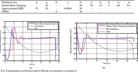
30 and 150 degree initial angles in pitch plan and target has -3g maneuver. Therefore, target is coming and initial range is 40 km. The other parameters are as listed in Table 1.

In this scenario, commanded and missile lateral acceleration, line of sight rate and relative lateral velocity is plotted in Figs. 2 and 3.

As shown in figures, the missile acceleration is smooth and implementable in all guidance laws. The precision of controlling line of sight rate and relative lateral velocity are higher than two other guidance laws. As shown in Figs.4 and 5, the interception time and velocity losses are lower than other guidance laws. In this scenario, it can be said; due to high relative range the missile has enough time for reactions and the control loop dynamics does not have very bad influences on guidance loop.

Table 1 The values of parameters in scenario I.

Guidance Law η μ N ε At k1 k2 k3 γ1 γ2

Robust Back-Stepping - 30 - - 30 30 10 5 0.8 0.4

Approximated SMG 70 30 - 0.0008 30 - - - - -

TPNG - - 4 - 30 - -

0 5 10 15 20 25 30

-70 -60 -50 -40 -30 -20 -10 0

Time (s)

C

o

m

a

n

d

e

d

A

c

e

le

ra

ti

o

n

(

m

/s

2)

Robust Back Stepping Guidance SM Guidance

TPN

0 5 10 15 20 25 30

-70 -60 -50 -40 -30 -20 -10 0

Time (s)

M

is

s

ile

A

c

e

le

ra

ti

o

n

(

m

/s

2)

TPN

(a) (b)

Fig. 2 a) Commanded acceleration and b) Missile acceleration in scenario I.

0 5 10 15 20 25 30

-0.8 -0.7 -0.6 -0.5 -0.4 -0.3 -0.2 -0.1 0 0.1

Time (s)

L

O

S

R

a

te

(

d

e

g

/s

)

TPN

0 5 10 15 20 25 30

-200 -150 -100 -50 0 50

Time (s)

R

e

la

ti

v

e

L

a

te

ra

l

V

e

lo

c

it

y

(

m

/s

)

TPN

(a) (b)

Fig. 3 a) Line of sight rate and b) Relative lateral velocity in scenario I.

(6)

Design a Guidance Law Considering Approximation of Missile Control Loop Dynamics Using Adaptive Back-Stepping Theory

… V. Behnamgol, A. R. Vali and A. Mohammadi

0 1

2

3 4 x 104 -1

-0.5 0 0.5 1 -4000 -2000 0 2000 4000

X(m) Y(m)

Z

(m

)

TPN

Target Trajectory

0

0.5

1

1.5 2

2.5

3

3.5 4

x 104

-1 -0.8 -0.6 -0.4 -0.2 0 0.2 0.4 0.6 0.8 1 -3000 -2000 -1000 0 1000 2000

X(m)

TPN Target Trajectory

Fig. 4 Missile and target trajectories in scenario I.

0 5 10 15 20 25 30

900 1000 1100 1200 1300 1400 1500

Time (s)

C

lo

s

in

g

V

e

lo

c

it

y

(

m

/s

)

TPN

Fig. 5 Closing velocity in scenario I.

5.2 Scenario II

In second scenario missile and target is flying with 0 and 150 degrees angles in pitch plan, respectively. Target has 2g maneuver. Therefore, target is going and initial relative range is 10 km. the values of parameters in this scenario are as listed in Table 2.

In this scenario, commanded and missile lateral acceleration, line of sight rate and relative lateral acceleration are plotted in Figs. 6 and 7. As illustrated in these figures, the missile accelerations are smooth and implementable. By applying proposed guidance law, the line of sight rate and relative lateral velocity are converging to zero and these variables are not controlled using two other guidance laws. As shown in Figs.8 and 9 the missile intercept to target by using proposed guidance law , but the closing velocity reaches to zero and guidance loop is instable by using other guidance laws.

In this case, the miss distance is 46 and 21 m by using approximated sliding mode and proportional guidance laws, respectively. Therefore, in this scenario that the relative range is shorter than first scenario, the control loop dynamics leads to instability by using approximated sliding mode and proportional guidance

laws.

6 Conclusions

In this paper, a guidance law considering approximation of control loop dynamic is designed using robust back-stepping theory. In the guidance loop, the missile-target relative kinematics is considered as a control process. The control input is the commanded acceleration and the output is the relative lateral velocity based on parallel navigation idea. In this guidance loop, the missile control loop act as an actuator and implement the guidance commands. The dynamics of this section commonly is not to be considered in designing guidance law and it is neglected. But for increasing precision, the approximation of missile control loop dynamics is added to kinematics equations and then the guidance law is designed. The simulation results show that the missile control loop dynamics can cause instability in older guidance laws such as approximated sliding mode and pure proportional guidance laws; but the proposed robust back-stepping guidance law has appropriate performance in the presence of missile control loop dynamics.

(7)

Table 2 The values of parameters in scenario II.

Guidance Law η μ N ε At k1 k2 k3 γ1 γ2

Robust Back-Stepping - 20 - - 20 30 10 5 0.7 0.1

Approximated SMG 10 20 - 0.00003 20 - - - - -

TPNG - - 4 - 20 - -

0 1 2 3 4 5 6 7 8

-300 -200 -100 0 100 200 300

Time (s)

C

o

m

a

n

d

e

d

A

c

e

le

ra

ti

o

n

(

m

/s

2)

TPN

0 1 2 3 4 5 6 7 8

-150 -100 -50 0 50 100 150

Time (s)

M

is

s

ile

A

c

e

le

ra

ti

o

n

(

m

/s

2)

TPN

(a) (b)

Fig. 6 a) Commanded acceleration and b) Missile acceleration in scenario II.

0 1 2 3 4 5 6 7 8

-3 -2 -1 0 1 2 3

Time (s)

L

O

S

R

a

te

(

d

e

g

/s

)

TPN

0 1 2 3 4 5 6 7 8

-400 -300 -200 -100 0 100 200 300 400 500

Time (s)

R

e

la

ti

v

e

L

a

te

ra

l

V

e

lo

c

it

y

(

m

/s

)

TPN

(a) (b)

Fig. 7 a) Line of sight rate and b) Relative lateral velocity in scenario II.

0

5000

10000 -1

0 1

0 1000 2000 3000

X(m) Y(m)

Z

(m

)

TPN

Target Trajectory

0 1000

2000 3000

4000 5000

6000 7000

8000 9000

10000

-1 -0.8 -0.6 -0.4 -0.2 0 0.2 0.4 0.6 0.8 1 0 500 1000 1500 2000 2500

X

(m

)

Fig. 8 Missile and target trajectories in scenario II.

(8)

<

0 1 2 3 4 5 6 7 8

0 500 1000 1500

Time (s)

C

lo

s

in

g

V

e

lo

c

it

y

(

m

/s

)

TPN

7 7.1 7.2 7.3 7.4 7.5

0 50 100 150 200 250 300 350 400

Time (s)

R

e

la

ti

v

e

R

a

n

g

e

(

m

)

TPN

(a) (b)

Fig. 9 a) Closing velocity and b) Relative range in scenario II.

References

[1] G. M. Siouris, Missile Guidance and Control

Systems. Springer, 2005.

[2] P. Zarchan, Tactical and Strategic Missile

Guidance. AIAA Series, Sixth Edition, Vol. 239,

2012.

[3] R. Yanushevsky, Modern Missile Guidance. Taylor & Francis Group, 2008.

[4] N. A. Shneydor, Missile Guidance and Pursuit:

Kinematics, Dynamics and Control. Horwood

Publishing, 1998.

[5] R. Yanushevsky and W. Boord, “Lyapunov approach to guidance laws design,” Nonlinear

Analysis, Vol. 63, pp. 743–749, 2005.

[6] D. Zhou, Sh. Sun and K. L. Teo, “Guidance Laws with Finite Time Convergence,” Journal of

Guidance, Control, and Dynamics, Vol. 32, No. 6,

pp. 1838–1846, 2009.

[7] K. R. Babu, I. G. Sarma and K. N. Swmy, “Switched Bias Proportional Navigation for Homing Guidance Against Highly Maneuvering Target,”

Journal of Guidance, Contro1, and Dynamics,

Vol. 17, No. 6, pp. 1357–1363, 1994.

[8] M. Innocenti, “Nonlinear guidance techniques for agile missiles,” Control Engineering Practice, Vol. 9, pp. 1131–1144, 2001.

[9] J. Moon, K. Kim and Y. Kim, “Design of Missile Guidance Law via Variable Structure Control,”

Journal of Guidance, Control, and Dynamics,

Vol. 24, No. 4, pp. 659–664, 2001.

[10]T. Binazadeh and M. J. Yazdanpanah, “Partial Stabilization Approach to 3-Dimensional Guidance Law Design,” Journal of Dynamic Systems,

Measurement, and Control, Vol. 133, 2011.

[11]T Binazadeh and M-J Yazdanpanah, “Robust partial control design for non-linear control systems: a guidance application,” Systems and Control

Engineering, Vol. 225, 2011.

[12]F. K. Yeh, K. Y. Cheng and L. Ch. Fu, “Variable

Structure-Based Nonlinear Missile

Guidance/Autopilot Design with Highly

Maneuverable Actuators,” IEEE Transactions on

Control Systems Technology, Vol. 12, No. 6,

pp. 944–949, 2004.

[13]M. Xin, S. N. Balakrishnan and E. J. Ohlmeyer, “Integrated Guidance and Control of Missiles With Teta-D Method,” IEEE Transactions on Control

Systems Technology, Vol. 14, No. 6, pp. 981–992,

2006.

[14]B. S. Kim, A. J. Caliset and R. J. Sattigeri, “Adaptive, Integrated Guidance and Control Design for Line-of-Sight-Based Formation Flight,” Journal

of Guidance, Control, and Dynamics, Vol. 30,

No. 5, pp. 1386–1398, 2007.

[15]A. Koren and M. Idan, “Integrated Sliding Mode Guidance and Control for Missile with on-off Actuators,” Journal of Guidance, Control, and

Dynamics, Vol. 31, No. 1, pp. 204–213, 2007.

[16]Y. B. Shtessel, I. A. Shkolnikov and A. Levant, “Guidance and Control of Missile Interceptor using Second-Order Sliding Modes,” IEEE Transactions

on Aerospace and Electronic Systems, Vol. 45,

No. 1, pp. 110–124, 2009.

[17]Y. B. Shtessel and Ch. H. Tournes, “Integrated Higher-Order Sliding Mode Guidance and Autopilot for Dual-Control Missiles,” Journal of Guidance,

Control, and Dynamics, Vol. 32, No. 1, pp. 79–94,

2009.

(9)

Iranian Journal of Electrical & Electronic Engineering, Vol. 14, No. 3, September 2018 212 [18]S. S. Vaddi, P. K. Menon and E. J. Ohlmeyer,

“Numerical State-Dependent Riccati Equation Approach for Missile Integrated Guidance Control,”

Journal of Guidance, Control, and Dynamics,

Vol. 32, No. 2, pp. 699–703, 2009.

[19]C. L. Lin, H. Z. Hung, Y. Y. Chen and B. S. Chen, Development of an integrated fuzzy-logic-based missile guidance law against high speed target, IEEE

Transaction on Fuzzy Systems, Vol. 12, No. 2, 157–

169, 2004.

[20]J. H. Chen, Y. A. Zhang and J. Y. Yu, “Lyapunov Stability Based Guidance Law Considering Compensation to Dynamics of Missile,” in Proceedings of the Fourth International Conference

on Machine Learning and Cybernetics, Guangzhou,

Aug. 2005.

[21]D. R. Taur, “A Sliding Mode Nonlinear Guidance with Navigation Loop Dynamics of Homing Missiles,” AIAA Guidance, Navigation, and Control

Conference, Toronto, Canada, Aug. 2010.

[22]Sh. Sun, D. Zho and W. Hou, “A guidance law with ﬁnite time convergence accounting for autopilot lag,” Aerospace Science and Technology, Vol. 25, pp. 132–137, 2013.

[23]Y. B. Shtessel, I. A. Shkolnikov and A. Levant, “Smooth second-order sliding modes: Missile guidance application,” Automatica, Vol. 43, pp. 1470 – 1476, 2007.

V. Behnamgol was born in Iran in 1985. He received the B.Sc. degree from Shomal University, Amol, Iran, in 2009, and the M.Sc. degree from Malek Ashtar University, Tehran, Iran, in 2011, all in Electrical Engineering. He is currently a Ph.D. student of Control Engineering at the Malek Ashtar University of Technology of Tehran, Iran. He has authored more than 20 scientiﬁc journal and conference papers. His research interests include nonlinear, sliding mode and robust control and guidance systems.

A. R. Vali was born in Iran in 1972. He received the B.Sc. degrees in Electrical Engineering from the Shiraz University, Shiraz, Iran, in 1995 and M.Sc. and Ph.D. degrees of Department of Electrical Engineering, Amir Kabir University of Technology, Tehran, Iran, in 1998 and 2005, respectively. He is the author of more than 30 journal and conference papers in the field of nonlinear control systems, analysis and control of time delay systems, tracking systems, modeling and control of biological systems, guidance and control and robotics. Dr. Ahmad Reza Vali is currently Associate Professor at Department of Control Engineering, Malek Ashtar University of Technology, Tehran, Iran.

A. Mohammadi was born in Iran. He received the B.Sc. M.Sc. and Ph.D. degrees in Electrical Engineering from the Sharif University of technology, Tehran, Iran. He is the author of more than 30 journal and conference papers in the field of control systems and estimation. Dr. Ali Mohammadi is currently Assistant Professor at Department of Control Engineering, Malek Ashtar University of Technology, Tehran, Iran.

access article distributed under the terms and conditions of the Creative

Commons Attribution-NonCommercial 4.0 International (CC BY-NC 4.0)

license (https://creativecommons.org/licenses/by-nc/4.0/).

Downloaded from ijeee.iust.ac.ir at 14:48 IRDT on Friday September 18th 2020 [ DOI: 10.22068/IJEEE.14.3.204 ]