www.astesj.com 192
MIMO Performance and Decoupling Network: Analysis of Uniform Rectangular array Using
Correlated-Based Stochastic Models
Obour Agyekum Kwame O-B*, Maxwell Oppong Afriyie1, Paul Oswald Kwasi Anane1, Affum Emmanuel Ampoma1, Matthew
Seddoh Akatey2
1University of Electronic Science and Technology of China, School of Communication and Information Engineering, 611731, China 2University of Electronic Science and Technology of China, School of Energy Science, 611731, China
A R T I C L E I N F O A B S T R A C T Article history:
Received: 18 December, 2016 Accepted: 21 January, 2017 Online: 28 January, 2017
We explore the dependency of MIMO performance on azimuthal spread (AS) and elevation spread (ES) using correlated-based stochastic models (CBSMs). We represent the transmitter as uniform rectangular array (URA), and derive an analytical function for spatial correlation, in terms of maximum power when phase gradient of the incident wave follows a Student’s t-distribution. We model the correlated-based stochastic MIMO system to investigate the usefulness of the analytical function, under the condition that the magnitude and phase of mutual coupling and consequently the coupling matrix of the coupled receiving monopole array differs much from that of the decoupled array. Verification is achieved with the help of simulation results, which support the existing fact that the azimuthal spread is the fundamental determinant of system capacity. However, we observed that lower values of AS and ES increase the rate of deterioration in the symbol error rate (SER) and not antenna spacing after decoupling process.
Keywords:
Azimuthal Spread (AS) Decoupling Network Elevation Spread (ES) Mutual coupling (MC) Spatial Correlation Function Uniform Rectangular Array (URA)
1. Introduction
The correlation-based stochastic models (CBSMs) are mainly used for theoretical analysis to assess the performance of massive MIMO systems. However, these models could be applied to cases where the user equipment (UE) with multiple antennas works at millimeter wave [1]. Although the fifth generation (5G) wireless communication technology will offer alluring features such as higher transmission rate, there are still several challenges ahead in the deployment of this technology [2-3]. Very recently, antenna arrays have attracted attention in the wireless communication industry to enhance signal quality, coverage and capacity. This is because antenna configuration directly influences the channel characteristics and performance, therefore, it is a critical factor in deciding the channel characteristics in MIMO technology.
In view of this, all attempts to improve the performance of the existing MIMO technology must be investigated especially in regards to realistic channel models.
All endeavours to improve and enhance the performance of the existing MIMO technology need to be explored, specifically with regards to analyzing the MIMO characteristics of wireless channels.
The authors in [4] demonstrated that having the MIMO system in three dimensional view is the efficient method for managing spatial resource. Several array configurations have been the subject of investigations on MIMO technology, and most of the prior investigations considered simple system configurations using only AS [5–9].
Many refer to the work in [8] and [9] where researchers presented spatial correlation function for four-element receiving circular arrays, when the angle-of-arrival (AoA) followed Laplacian and truncated Gaussian distributions respectively, because the uniform circular array (UCA) configuration has been the subject of many investigations on MIMO technology. Although the authors derived the correlation function for UCA in terms of AS by considering that the ES of the incoming plane wave in the propagation geometry is 90o, their contribution provides fundamental basis for evaluating
the spatial correlation function of URA in advanced MIMO technologies. Therefore, our objective in this paper is to experiment the CBSMs at 2.4 GHz. We modelled the transmitter as a uniform rectangular array, and examined the effects of spatial fading correlation and mutual coupling on channel capacity and symbol error rate (SER). To prove our concept, we quantify the mutual coupling of the receiving array by the receiving mutual impedance method (RMIM) [10], whereas, we examined the URA in the CST
ASTESJ
ISSN: 2415-6698*Corresponding Author: Obour Agyekum Kwame O-B, University of Electronic
Science and Technology of China, 611731, China Email: [email protected]
www.astesj.com
Special Issue on Computer Systems, Information Technology, Electrical and Electronics Engineering
Microwave Studio to determine the coupling matrix. Recently, authors in [11] proposed a spatial correlation function for MIMO channel model on the latest 3GPP standards and WINNER+ [12]. We are of the view that our concept will add to cover new aspects in MIMO modelling studies.
For purposes of clarity, the contributions in this paper are as follows: 1) We fabricate a decoupling network to study the dependence of system performance on antenna spacing, AS and ES of MIMO system, using CBSMs on the assumption that the magnitude and phase of the mutual coupling and consequently the coupling matrix of the coupled array varies from that of the decoupled array at the receiving end. 2) We derive an analytical expression for spatial correlation function of a URA, based on maximum power in the direction of maximum arrival using the Student’s t-distribution. 3) Our outcomes show that azimuthal spread (AS) is the essential determinant of system performance. Also, lower values of AS and ES increase the rate of deterioration in the SER, and not antenna spacing.
This letter is organized as follows: Section II presents the design of the decoupling network. In Section III, we derive the closed-form expression for the spatial correlation function in terms of maximum power for URA using Student’s t-distribution. Section IV presents analytical and simulation results. Finally, we give concluding remarks in Section V.
2. Operating Matrix of the Decoupling Network
The compensation network is designed using a power-divider and two rat-race couplers. The power divider has unequal power-dividing ratio with no active circuit elements to minimize extra circuit noise. The operating matrix for two-element receiving array is given by [13].
12 12
1 2
1 1
2 21 2 21
2 1
1
1
L L
L L
Z Z
V V
Z Z
U V
U Z V Z
V V
Z Z
(1)
where the inputs to network are coupled voltages V1 and V2 from the two monopole antennas, and the outputs of network are compensation voltages U1 and U2. The mutual impedance between the two monopole antennas is represented by Z12 and ZL is the matched load impedance. In order to achieve the tri-band operation, we utilized resonators and stubs.
By sharing the stub with the resonator (parallel LC circuit) of two adjacent
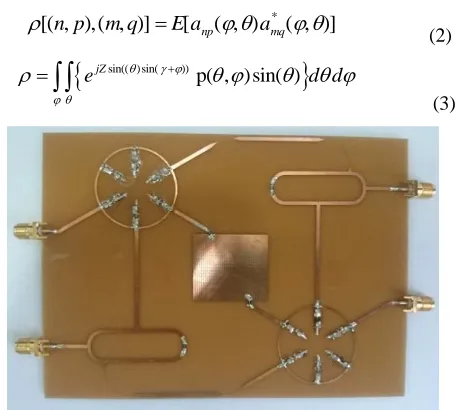
-shaped structure circuits within the rat-race couplers, a decoupling network with working frequencies 2.4/3.5/5.5 GHz was designed. The length and impedance of stubs at different frequencies are calculated using the procedure in [14]. The decoupling network has been designed using ADS and fabricated using FR4 substrate with dielectric constant 4.8 as shown in Fig. 1. Simulated and measured responses are shown in Fig. 2. Measured results at 2.4/3.5/5.5 GHz demonstrate that isolation and insertion losses between input and output ports of more than 10 dB can be accomplished. To achieve best performance, the initial values of the impedance and the parallel resonator had to be increased to accomplish the tri-band operation. This accounted for the large differences between simulated and measured values in Fig. 2(a) and Fig. 2(b) at 3.5 GHz.3. System Model
3.1.Proposed Spatial Correlation of URA
The spatial correlation between antennas at positions ( , )n p and ( , )m q following the procedure in [14] is expressed as
*
[( , ),( , )]n p m q E a[ np( , )amq( , )]
(2)
sin(( )sin( ))
p( , )sin( )
jZ
e d d
(3)
Fig. 1. Photograph of the fabricated compensation network
2.0 2.5 3.0 3.5 4.0 4.5 5.0 5.5 6.0 -70
-60 -50 -40 -30 -20 -10 0
Ma
gnitude (dB)
Freqeuncy (GHz)
M_S22 S_S22 M_S11 S_S11 M_S21 S_S21
2.0 2.5 3.0 3.5 4.0 4.5 5.0 5.5 6.0 -60
-50 -40 -30 -20 -10 0
Magnitude (dB)
Frequency (GHz)
S_S32 M_S32 M_S42 S_S42
2.0 2.1 2.2 2.3 2.4 2.5 2.6 -30
-24 -18 -12 -6 0
Magni
tude
(dB)
Freqeuncy (GHz)
S_S31 M_S31
S_S41 M_S41
2.0 2.5 3.0 3.5 4.0 4.5 5.0 5.5 6.0 -70
-60 -50 -40 -30 -20 -10 0
Mag
nitu
de
(dB)
Frequency (GHz) M_S44 M_S33
S_S44 S_S33
S_S43 M_S43
Fig. 2. Simulated and measured scattering parameters of the decoupling network for (a) input ports, (b), (c) input and outputs ports, and (d) output ports.
where p( , ) is the joint spatial power spectrum. For our theoretical analysis, we have used the fact that the maximum power
in the direction of maximum arrival is proportional top( , ) . Therefore, we represent the joint spatial power spectrum p( , ) in (3) by the maximum power Pt( ) of the incident plane wave and proportional to AS and ES. If the phase gradient has a Student’s t-distribution as in [15], compared to the choice of joint spatial power spectrum of [14], then the phase in (3) can be expressed as
sin( ) Zk
2
3/ 22 2
( ) 1 2 cos( ) sin sin( )
p
s
s
(4)
wheres is the measure of angular spread. In our analysis we
assumed that
2 2
sin sin sin
. The maximum power
( ) t P
in the direction of maximum arrival isPt( )
p( ) d . With the above assumptions, we can rewrite (3) as
sin( )sin( )]
( ) sin( )
t
jZ
P e d d
(5)
4 Z P
t( )sin( ) Z (6) A. Theoretical and S-parameter based mutual couplingIncorporating the effect of mutual coupling, the channel vector can be written as follows
1/2
m o
H
Z
H
(7)
m
Z
and
denote the coupling and spatial correlation matrices at the receiver and transmitter respectively. The theoretical approximation of coupling matrix is expressed as
1
12
(
)(Z
)
M A L L
Z
Z
Z
Z I
(8)
where ZA,ZL,Z12 are the antenna, load and mutual impedances
respectively. With the above assumption that the magnitude and phase of the mutual coupling are different, we used RMIM measurement procedure shown in Fig. 3 to evaluate the mutual coupling between small receiving monopole arrays at the receiving end under two conditions [10] describe in Section IV. The mutual
impedance Z12is expressed as [10]
(1) ( 2)
11 21 21
12
Z
S
S
S
ZL(9)
where S11 is the measured scattering parameter at monopole 1’s
terminal with monopole 2 removed (taken away from the array),
(1)
21 S
is the measured scattering parameter at monopole 1’s terminal
with monopole 2’s terminal connected toZLand
( 2 )
21 S
defines the measured scattering parameter at monopole 2’s terminal with
monopole 1’s terminal connected toZL Moreover, in terms of scattering parameters [16] coupling matrix in (7) is given as
1
(
t)(
t)
LM
Z
I
S
I
S
Z
(10)
where matched load impedance
Z
L has a value of50
and N Nt S M
is the S-parameter matrix of the antenna array. To determine the S-parameters at the transmitting end, the URA is modelled in CST Microwave Studio as a
4 4
monopole array, located in the xyplane.Fig. 3. Measuremwnt of receiving mutual impedance in anechoic chamber at 2.4 GHz
4. Numerical Results
In this section, we present the analytical performance and the simulation results of MIMO system using CBSMs. We modelled and analyzed the correlated-based stochastic MIMO channel, based on the two conditions that the magnitude and the phase of the mutual coupling and the coupling matrix of the coupled receiving array vary much from that of the decoupled array. The simulated channel is according to (6)-(10) and it is assumed that fading is correlated at both transmitter and receiver sides. The receiving array is represented by two-monopole element on a metallic ground and operating at 2.4 GHz. The monopoles have length of 30 mm, radius of 0.5 mm and element separation of/ 8. As indicated already, the formulation of coupling matrix of the receiving array is determined in anechoic chamber under two conditions using RMIM.
Condition I: the S-parameters of the coupled array are determined
to estimate for the coupled voltages (V1andV2 ), and also to
formulate the coupling matrix using (9)-(10).
Condition II: the monopole array is connected to the decoupling network through equivalent length coaxial links. The scattering parameters of the output ports of the decoupling network are determined to formulate the coupling matrix and estimate for the
compensated voltages (U1andU2).
With the end goal of justifying the assumption that the magnitude and phase of mutual coupling of coupled array differs much from the decoupled array at the receiving end, there are three different types of voltages recorded in Table I. The last row in Table I is a ratio of the voltage obtained with monopole B to the voltage obtained with monopole A. It can be seen that the ratio of the compensated voltage is very close to the uncoupled voltages. This also demonstrates that the compensated voltages have successfully
been removed off the coupling effect. The value of
is determined for each antenna spacing of the URA and incorporated into the channel model.4.1.Effects of AS and ES- Performance Tradeoff
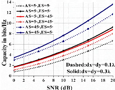
modelling of coupling capacity matrix at the receiving side in Fig. 4 and Fig. 5 support the existing fact of the effects of higher values of azimuthal spread (AS) on system performance. Our outcomes demonstrate that elevation spread (ES) does not affect system capacity as much as the azimuthal spread (AS) does. Moreover, it is therefore not surprising that spacing between antenna elements affects system performance. However, larger number of transmit antennas improve system performance in a fixed physical space.
4.2.Symbol error rate (SER) vs SNR
In Fig. 6, there is a close match between symbol error rate (SER)
for ASES30 at 0.2 and 0.5respectively. We observed that the SER after an increase of 10dB forAS45 , ES20 at 0.5 remains nearly the same as that forAS20 ,ES45 at 0.2. A close inspection of Fig. 6 reveals that the impacts of higher values of AS and antenna spacing on the channel capacity are more significant than SER. We note that lower values of AS and ES increase rate of deterioration in the SER and not antenna spacing after decoupling process.
Fig. 4. Capacity vs SNR for antenna spacing 0.1
and 0.3
Fig. 5. Capacity vs SNR for antenna spacing 0.2
and 0.5
Fig. 6. SER vs SNR for QPSK with 4 4 URA Table 1: Different Measured Voltages
Uncoupled Voltages (reference)
Coupled voltages
Compensated voltages
M
o
n
o
p
o
le
A mag (mV) 16.64 12.4 11.55
angle (
) -160.64 -166.67 34.967M
o
n
o
p
o
le
B
mag (mV) 16.54 15.42 12.30
angle (
) -139.56 -141.46 55.16B/A mag (mV) 0.9939 1.2199 1.065
angle (
) 21.08 25.208 20.1935. Conclusion
We derived an expression for the spatial fading correlation of URA when the phase gradient follows Student’s t-distribution. We investigated dependency of MIMO performance on azimuthal spread (AS) and elevation spread (ES) after decoupling process using CBSMs. Our results support the existing fact that the azimuthal spread (AS) is the essential determinant of system performance. Additionally, results confirm that lower estimations of AS and ES significantly expand the rate of deterioration in the SER, and not antenna element separation after decoupling process.
Appendix
The integral in (5) is evaluated in this appendix. Using the properties of Bessel function in the case of n0 as [17]
( sin( ))
1 ( )
2 n
j n x
J x e d
0
sin( )
1 2 n
jx
e d
0
2 2
cos( ) 1
2
jx u
e du
we can rewrite (5) as
2
0 0
cos( )
( ) sin( ) jx
t
P e d d
(12)where xZsin( ) . Using specific solutions in (11) such as
0
1
0 2
( )
( sin( )) sin( ) 2
x
o J x
J x d x
(13)
and
1 2
0 2
( )
sin( )
x
x
J
x
x
, we obtain (6). To evaluate
( )
( )
t
P
p
d
, we use the series [18]
2 2 2 2
2 2
(cos ) (1 sin ) (1 sin )
sin (1 sin )
sin 2
1 2
d
n
Using the series
2 11
1 /
1
ln( )
2
1
n
n
n
and
1 2
2 0
2 2
1
( 1) cos( )
2
n
n n k
n k
n n
Sin n k
k n
(14)with well-known Taylor series of
cos
andsin
, (6) converges rapidly for small values ofZ
.References
[1] Kan Zheng, Suling Ou and Xuefeng Yin "Massive MIMO Channel Models: A Survey "International Journal of Antennas and Propagation”, vol. 2014, Article ID: 848071, Jun. 2014.
[2] Asvin Gohil, Hardik Modi and Shobhit K Patel “5G Technology of Mobile Communication: A Survey, IEEE Conference on Intelligent Systems and Signal Processing (ISSP), pp. 288 – 292, March 2013.
[3] Kan Zheng, Suling Ou and Xuefeng Yin “Massive MIMO Channel Models: A Survey”, International Journal of Antennas and Propagation, vol. 2014, Article ID 848071, June 2014.
[4] Jianhua Zhang, Chun Pan, Feng Pei, Guangyi Liu, and Xiang Cheng "Three-Dimensional Fading Channel Models: A Survey of Elevation Angle Research,” IEEE Communications Magazine, June 2014, pp. 218-226 [5] J. Zhou, S. Sasaki, S. Muramatsu, H. Kikuchi, and Y. Onozato, “Spatial
correlation for a circular antenna array and its applications in wireless communication,” in IEEE Global Telecommunications Conference, GLOBECOM ’03., vol. 2, Dec 2003, pp. 1108–1113.
[6] A. Forenza, D. J. Love, and R. W. Heath, “Simplified spatial correlation models for clustered MIMO channels with different array configurations,” IEEE Transactions on Vehicular Technology, vol. 56, no. 4, July. 2007, pp.1924–1934.
[7] J.-A. Tsai and B. Woerner, “The fading correlation function of a circular antenna array in mobile radio environment,” in IEEE Global Telecommunications Conference, vol. 5, May 2001, pp. 3232–3236. [8] Jiann-An Tsai, R. Michael Buehrer, and Brian D. Woerner “BER Performance
of a Uniform Circular Array versus a Uniform Linear Array in a Mobile Radio Environment”, IEEE Transactions on Wireless Communications, vol. 3, No. 3, May 2004, Page: 732.
[9] Jiann-An Tsai, R. Michael Buehrer “Spatial Fading Correlation Function of Circular Antenna Arrays With Laplacian Energy Distribution”, IEEE Communications Letters, vol. 8, No. 5, May 2002, Page: 295
[10] H. T. Hui, “A new definition of mutual impedance for application in dipole receiving antenna arrays,” IEEE Antennas Wireless Propag. Lett. vol. 3, pp. 364–367, 2004.
[11] Qurrat-Ul-Ain Nadeem, Abla Kammoun, M'erouane Debbah†, and Mohamed-Slim Alouini "Spatial Correlation Characterization of a Uniform Circular Array in 3D MIMO Systems,” International Workshop on Signal Processing Advances in Wireless Communications (SPAWC), July 2016, pp: 1 - 6
[12] 3GPP TR 36.873 V12 .0.0, “Study on 3D channel model for LTE,” Sep.2014 [13] Y. Yu and H.T. Hui "Design of a Mutual Coupling Compensation Network for a Small Receiving Monopole Array", IEEE Trans. On Micro. Theory and Techniques, vol. 59, no. 9, pp. 2241-2245, Sept. 2011.
[14] S. K. Yong and J. S. Thompson, “A three-dimensional spatial fading correlation model for uniform rectangular arrays”, IEEE Antennas and Wireless Propag. Lett, vol. 2, no. 1, pp. 182–185, 2003.
[15] J. B. Andersen and K. I. Pedersen, “Angle-of-arrival statistics for low resolution antenna”, IEEE Trans. Antennas Propagat. vol. 50, No. 3, pp.391-395, Mar. 2002.
[16] D. Masouros, J. Chen, K. Tong, M. Sellathurai, and T. Ratnarajah, “Towards massive-MIMO transmitters: on the effects of deploying increasing antennas in fixed physical space,” in Proc. of the Future Network and Mobile Summit, pp. 1–10, 2013.
[17] Abramowitz Milton, Stegun Irene “Handbook of Mathematical Functions with Formulas, Graphs and Mathematical Tables”, New York: Dover, ISBN 0-486-61272-4.