Parameters Sensitivity Characteristics of Highly Integrated Valve-Controlled Cylinder Force Control System

ORIGINAL ARTICLE

Parameters Sensitivity Characteristics

of Highly Integrated Valve-Controlled Cylinder

Force Control System

Kai‑Xian Ba

_{, Bin Yu}

_{, Xiang‑Dong Kong}

_{, Chun‑He Li}

_{, Qi‑Xin Zhu}

_{, Hua‑Long Zhao}

_{and Ling‑Jian Kong}

Abstract

Nowadays, a highly integrated valve‑controlled cylinder (HIVC) is applied to drive the joints of legged robots. Although the adoption of HIVC has resulted in high‑performance robot control, the hydraulic force system still has problems, such as strong nonlinearity, and time‑varying parameters. This makes HIVC force control very difficult and complex. How to improve the control performance of the HIVC force control system and find the influence rule of the system parameters on the control performance is very significant. Firstly, the mathematical model of HIVC force control system is established. Then the mathematical expression for parameter sensitivity matrix is obtained by apply‑ ing matrix sensitivity analysis (PSM). Then, aimed at the sinusoidal response under (three factors and three levels) working conditions, the simulation and the experiment are conducted. While the error between the simulation and experiment can’t be avoided. Therefore, combined with the range analysis, the error in the two performance indexes of sinusoidal response under the whole working condition is analyzed. Besides, the sensitivity variation pattern for each system parameter under the whole working condition is figured out. Then the two sensitivity indexes for the three system parameters, which are supply pressure, proportional gain and initial displacement of piston, are proved experimentally. The proposed method significantly reveals the sensitivity characteristics of HIVC force control system, which can make the contribution to improve the control performance.

Keywords: Highly integrated valve‑controlled cylinder system, Force control system, Matrix sensitivity analysis, Orthogonal test design, Sensitivity index

© The Author(s) 2018. This article is distributed under the terms of the Creative Commons Attribution 4.0 International License (http://creat iveco mmons .org/licen ses/by/4.0/), which permits unrestricted use, distribution, and reproduction in any medium, provided you give appropriate credit to the original author(s) and the source, provide a link to the Creative Commons license, and indicate if changes were made.

1 Introduction

The valve-controlled cylinder system is the most com-monly used component in the hydraulic system and is widely used in many fields such as aerospace, metal-lurgy, engineering machinery, agricultural machinery and advanced manufacturing. The highly integrated valve-controlled cylinder (HIVC) which has the high power density is used with unique advantages in the aerospace load simulator and the high performance legged robot which are different from the traditional civil equipment and require higher entire performance to ensure better adaptability under the complex environment. Therefore,

the lighter weight and the faster response are required for the HIVC, which makes the structure optimization and the compensation control method of the HIVC have

practical significance [1–5].

The control methods of the HIVC include the posi-tion control and the force control, and the posiposi-tion con-trol compared with the force concon-trol is more mature, yet the force control is widely applied to the heavy industry, the aerospace load simulator and the advanced manu-facturing. But the quantitative performance analysis and the system optimization method of the force control are less, and how to improve the force control performance effectively should be analyzed further. The force control is relied on the compressibility of the oil and is achieved through controlling the oil volume of the closed oil cav-ity, and ensuring the stability of the control component with small valve opening increases the force control

Open Access

*Correspondence: yb@ysu.edu.cn

1 _{School of Mechanical Engineering, Yanshan University,} Qinhuangdao 066004, China

difficulty and makes the effect of each system parameter on the force control system performance more sensi-tive. There are many parameters in the hydraulic system including structure parameters, working parameters and control parameters whose uncertainty caused by the manufacturing error, the testing error, the material aging, the non-ideal working condition and the online work-ing parameters fluctuatwork-ing makes the real workwork-ing per-formance no complete accordance to the ideal working performance, which is involved with what effect degree of the parameter change has on the force control perfor-mance. Therefore, it is needed to research which param-eter has greater effects on the force control performance and should be optimized and compensated and which parameter has smaller effects and can be ignored in the compensation control and structure optimization. The sensitivity analysis theory just can be applied to research the parameters change effects on the hydraulic system dynamic characteristics, and the sensitivity analysis results of the HIVC can be used to improve the system working performance, which would provide a novel idea for analyzing the system performance quantitatively and optimizing the compensation control method effectively, so the sensitivity analysis of HIVC force control system has significant theoretical research value and application prospects.

There are many sensitivity analysis methods includ-ing the matrix sensitivity analysis (MSA), the trajectory sensitivity analysis, the global sensitivity analysis, the variance-based sensitivity analysis and so on. All these sensitivity analysis methods have different mathemati-cal operation characteristics, so the operation accuracy, the operation style and the operation process are differ-ent, which makes each sensitivity analysis method have its own advantages and applied range. The MSA is based on the matrix operation that is applicable to the higher order hydraulic system even involved with many non-linear problems. Therefore, the MSA is adopted to ana-lyze the parameter sensitivity of the HIVC force control system. In recent years, the different sensitivity

analy-sis methods are applied to different fields. Ya et  al. [6]

adopted to trajectory sensitivity analysis research the correlation coefficients of random variables of mechani-cal structures, which provided guidance for the system

reliability researches. Abolfaz et  al. [7] adopted

trajec-tory sensitivity analysis to research the stability of under-ground rock structures, finding deep-influencing geo

mechanical parameters. Liu et al. [8] adopted trajectory

sensitivity analysis to research the structure parameters of the engine pipelines and demonstrated that some sup-ports’ positions played more important roles for complex piping, and the engine pipelines structure parameters

were optimized. Chatterjee et  al. [9] adopted trajectory

sensitivity analysis to found series and shunt compensa-tors in order to improve the transient stability of power

system. Song et al. [10] adopted global sensitivity

analy-sis to research the key parameters that affect model per-formance, and analyzed relationship between parameter identification, uncertainty analysis, and optimization in

hydrological modeling. Zheng et al. [11] adopted global

sensitivity analysis to perform on a marine ecosystem dynamic model, and proposed the model’s parameter optimization strategy and applied it to the Sanggou Bay.

Saltelli et al. [12] adopted variance-based sensitivity

anal-ysis to research the various available techniques for

sen-sitivity analysis of model output. Hall et al. [13] adopted

variance-based sensitivity analysis to give an incomplete picture of model response over the range of variability in the hydraulic model inputs, and shown that the variance-based sensitivity analysis is more general in its applicabil-ity and in its capacapplicabil-ity to reflect nonlinear processes and the effects of interactions among variables. Bashar et al.

[14] adopted MSA to research the performance

differ-ence between CPU and GPU in computer system. Billy

et  al. [15] adopted MSA to solve the steady-state

oper-ating point of regulator circuits and also examine the stability of operation in power system, and other meth-ods are compared in the performance of the steady-state determination and stability analysis. Zhang et  al.

[16] adopted MSA to research the electrical impedance

tomography by using the sensitivity matrix update, and the reconstructed images after sensitivity matrix update

were compared in power system. Naseralavi et  al. [17]

adopted MSA to research the structural damage detec-tion of cyclic structures.

Yet sensitivity analysis has a few applications in

hydrau-lic system. Vilenus [18] applied trajectory sensitivity

same working condition. Furthermore, Farasat et al. [19] founded the fourth order linear mathematical model of the valve-controlled cylinder position control system where the servo valve flow-pressure nonlinearity is lin-earized partially. The sensitivity of other parameters, such as servo valve torque motor constant, servo valve area constant, orifice opening of metering valve, system return oil pressure, supply oil volume, return oil volume and input signal voltage, is given with parameters change 1% under single working condition by four sensitivity evaluation methods including VILENUS method, revised VILENUS method, Entirety index method and Individual characteristics method. The analysis results indicated that the sensitivity of effective piston area of servo cyl-inder, flow coefficient, conversion mass and input signal

voltage is relatively small. Kong et al. [20–22] first

estab-lished the fifth linear order mathematical model for the hydraulic drive unit of quadruped robot and derived the first order trajectory sensitivity formulas analysis. Aimed at the imprecise conclusion of sensitivity analysis obtained from the linear model, some nonlinear models are also established. Besides, the sensitivity mathematical expressions with nonlinear and time-varied parameters are derived under the trotting gait working conditions.

Kong et al. [23] derived the mathematical model of the

second order trajectory sensitivity analysis based on the mathematical model of the first order trajectory sensitiv-ity formulas analysis. Therefore, the situation where the first order trajectory sensitivity formulas analysis accu-racy of some parameters is not high is improved. Then the experimental verification is conducted.

In Refs. [18–22], the hydraulic system sensitivity

anal-ysis was adopted to analyze the position control system and the mathematical model was simple even some of them.The trajectory sensitivity analysis method had the disadvantage of large computation, and the sensitivity results are obtained with only position step signal under one single working condition, which relatively decreased the reference value of the sensitivity results. However, the force control system is one of the main control methods of the HIVC and many problems need adopt the sensitiv-ity analysis to solve. What is the sensitivsensitiv-ity change rule of the force control parameters? How can the system parameters change influence the output response when the input signal is sinusoidal? What can the effects of each system parameter change have on the two perfor-mance indexes of sinusoidal response that are the ampli-tude attenuation and the phase lag which reflect on the control accuracy and response speed respectively? Which parameters change can improve or restrain the force control performance? How can the system parameters

sensitivity change under different working conditions? Especially, are the experimental results and the theoreti-cal analysis results coincident? With the above issues this paper is organized as follows: Firstly, the force control system mathematical model and the experimental system are described. Secondly, the MSA common mathemati-cal model and the appropriate MSA mathematimathemati-cal model for the HIVC are derived. Thirdly, working conditions are listed and nine working conditions based on the orthog-onal test design are selected to conduct the simulation analysis and the experiment research, and the dynamic change of the system parameters sensitivity is researched under these nine selected working conditions. Fourthly, the two sensitivity indexes based on the two performance indexes of sinusoidal response are derived, and the range analysis table based on the two sensitivity indexes is built to analyze the sensitivity value and change rules quantita-tively under the whole twenty-seven working conditions. Moreover, the effects of each parameter on the force con-trol performance and the methods to improve the force control performance are concluded. Finally, the sensitiv-ity analysis results are verified experimentally.

2 Introduction of HIVC 2.1 System Compositions

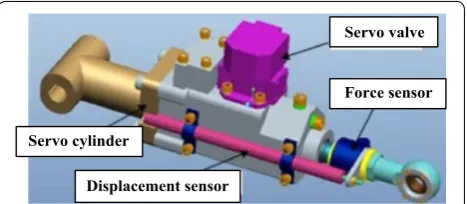
In this paper, the three-dimensional assembly drawing of

HIVC is shown in Figure 1 [24].

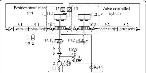
The performance test platform schematic of HIVC is

shown in Figure 2.

The performance test platform photo of HIVC is shown

in Figure 3.

In Figures 2 and 3, the right channel which consists of

small servo valve and servo cylinder is the tested HIVC controlled by the force-loop method, while the left chan-nel which consists of the same type servo valve and servo cylinder is the position simulation part controlled by the position-loop method. The two channels are connected by the cylinder piston rod, and displacement sensor and force sensor are installed in their joint.

Displacement sensor Servo cylinder

Force sensor Servo valve

2.2 Mathematical Model of HIVC Force Control System

The force control system transfer block diagram of HIVC

is shown in Figure 4.

In Figure 4, Kd = CdW

2

ρ , ω is natural frequency of

servo valve, ζ is damping ratio of servo valve, Cd is orifice

flow coefficient of spool valve, W is area gradient of spool

valve, ρ is density of hydraulic oil, Kd is conversion

coeffi-cient, ps is system supply oil pressure, p0 is system return

oil pressure, p1 is inlet cavity pressure of servo cylinder, p2

is outlet cavity pressure of servo cylinder, Cip is internal

leakage coefficient of servo cylinder, Cep is external

leak-age coefficient of servo cylinder, L is total piston stroke of

servo cylinder, L0 is initial piston position of servo cylinder,

Ap is effective piston area of servo cylinder, βe is effective

bulk modulus, mt is conversion mass(including the piston,

the displacement sensor, the force sensor, the connecting

pipe and the oil in servo cylinder), xp is servo cylinder

pis-ton displacement, xv is servo valve spool displacement, xr

is input displacement, Kaxv is servo valve gain, Kf is force

sensor gain, Kp is proportional gain, K is load stiffness, Bp is

viscous damping coefficient, F is output force, FL is external

load force, Vg1 is volume of input oil pipe, Vg2 is volume of

output oil pipe, Ff is friction, Ur is input voltage, Up is

dis-placement sensor feedback voltage, Ug is controller output

voltage, q1 is inlet oil flow, q2 is outlet oil flow. It can be seen

in Figure 4 that the highest order of system transfer block

diagram is sixth, and denote each vector in Table 1.

In Table 1, the state vector containing six state

vari-ables, input vector containing one input and parameter vector containing fourteen key parameters are selected,

Denote the expanded form of the state space Eq. (1)

including vectors in Table 1 as follows:

8.1

7 1.2

9.1 10.1 10.2 9.2 8.2

4

11.112 13 _11.2

U S

14.1 14.2

M15

6 5

2 1.1

3 M

1.316

U F

Controller Amplifier

Valve-controlled cylinder Position simulation

part

Controller Amplifier

Figure 2 Performance test platform schematic of HIVC. 1. Globe valve; 2. Axial piston pump; 3. Electromotor; 4. Relief valve 5. High‑ pressure filter; 6. Check valve; 7. Accumulator; 8. dSPACE controller; 9. Servo valve amplifier; 10. Servo valve; 11. Servo cylinder; 12. Displace‑ ment sensor; 13. Force sensor; 14. Electromagnetic valve; 15. Cooler; 16. Pressure meter

Displacement sensor Servo cylinder

Force sensor

Servo valve Accumulator

Figure 3 Performance test platform photo of HIVC

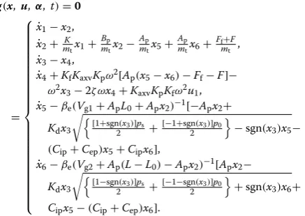
For the friction relative to the output force is small, so it is ignored in this paper. And denote the system

equa-tions including vectors in Table 1 as follows:

(1)                                                                              ˙

x1=x2,

˙

x2= −

K mt

x1−

Bp

mt

x2+

Ap

mt

x5−

Ap

mt

x6−

Ff+F

mt ,

˙

x3=x4, ˙

x4= −KfKaxvKpω2[Ap(x5−x6)−Ff−F]− ω2x3−2ζ ωx4+KaxvKpKfω2u1, ˙

x5=βe(Vg1+ApL0+Apx2)−1[−Apx2+

Kdx3

�

�_[1+sgn(x

3)]ps

2 +

[−1+sgn(x3)]p0 2

�

−sgn(x3)x5−

(Cip+Cep)x5+Cipx6], ˙

x6=βe(Vg2+Ap(L−L0)−Apx2)−1[Apx2−

Kdx3

� �

[1−sgn(x3)]ps

2 +

[−1−sgn(x3)]p0 2

�

+sgn(x3)x6+

Cipx5−(Cip+Cep)x6],

Y=Ap(x5−x6).

(2)

g(x,u,α,t)₌0

=                                                ˙ x1−x2, ˙ x2+_mK

tx1+

Bp

mtx2−

Ap

mtx5+

Ap

mtx6+

Ff+F

mt , ˙

x3−x4, ˙

x4+KfKaxvKpω2_{[Ap(x5−x6)−Ff−F]−} ω2x3−2ζ ωx4+KaxvKpKfω2u1, ˙

x5−βe(Vg1+ApL0+Apx2)−1[−Apx2+ Kdx3

� �_[1+sgn(x

3)]ps 2 +

[−1+sgn(x3)]p0 2

�

−sgn(x3)x5− (Cip+Cep)x5+Cipx6],

˙

x6−βe(Vg2+Ap(L−L0)−Apx2)−1[Apx2− Kdx3

� �_[1−sgn(x

3)]ps 2 +

[−1−sgn(x3)]p0 2

�

+sgn(x3)x6+ Cipx5−(Cip+Cep)x6].

The servo valve natural parameters are obtained from the servo valve product book which shows the fitted time domain and frequency domain characteristic curves. The structure parameters including effective piston area of servo cylinder, total piston stroke of servo cylinder and the volume of oil pipe are the factory data of the cylin-der. The working parameters including system supply oil pressure, system return oil pressure and sensor gain are taken from the experiment test, while other parameters are selected through engineering experience. Therefore, the force control system parameters and initial value of

HIVC are shown in Table 2.

3 MSA Mathematical Model 3.1 MSA Mathematical Common Model

Denote the common system equations as follows:

where x is m-dimensional state vector, u is r-dimensional

vector unrelated to α, α is p-dimensional vector and t is

time.

Initial value of the state vector x₀ can be obtained by

giving initial value of the input vector u0 and the initial

value of parameter vector α0, and initial state of Eq. (3)

are

(3)

g(x,u,α,t)=0,

(4)

g(x0,u0,α₀,t)=0.

Table 1 Each vector of the state space equations

State vector Input vector Output vector Parameter vector

x1=xp u1=Fr Y=F α1=ω α8=Ap

x2= ˙xp α2=ζ α9=βe

x3=xv α3=ps α10=mt

x4= ˙xv α4=p0 α11=Kf

x5=p1 α5=Cip α12=Kp

x6=p2 α6=L α13=K

α7=L0 α14=Bp

Table 2 Simulation model parameters and initial value

Simulation model parameters Initial value

Servo valve gain Kaxv (mm/v) 0.45 Natural frequency of servo valve ω (rad/s) 628 Damping ratio of servo valve ζ 0.77 Effective piston area of servo cylinder AP (mm2) 336.8 Volume of input oil pipe Vg1 (mm3) 620 Volume of output oil pipe Vg2 (mm3) 860 Total piston stroke of servo cylinder L(mm) 50 Initial piston position of servo cylinder L0 (mm) 20 System return oil pressure p0 (MPa) 0.5

Proportional gain KP 8

Force sensor gainKf(V/kN) 0.0769

External leakage coefficient Cep (mm3·(s·MPa)− 1) 0 Internal leakage coefficient Cip (mm3·(s·MPa)− 1) 238

Conversion mass mt(kg) 1.1315

Effective bulk modulus βe MPa 800

Load stiffness K(kN/m) 450

Denote Eq. (4) where input vector change Δu and

parameter vector change Δα causes the state vector

change Δx as follows:

Denote the Taylor expansion of Eq. (5) whose high

order Taylor expansions are ignored as follows:

Eq. (4) are taken into Eq. (6), the following is

Eq. (7) can be turned into

Define

and

Eqs. (9) and (10) are taken into Eq. (8), the following is

where S_α is m×p order parameter sensitivity matrix

(PSM) which contains time-varied elements, and Su is

m×r order input sensitivity matrix (ISM) which also

contains time-varied elements.

Denote the system output vector change as follows:

Based on Eq. (12) which is derived by MSA, the

approx-imate result of the output vector change ∆Y caused by

the parameter vector change α and input vector change

Δu can be obtained after the PSM Sα and ISM Su are

taken into Eq. (12).

3.2 MSA Mathematical Model of HIVC

In HIVC, the matrix in Eq. (7) is ∂g

∂x , which can be

expressed 6 × 6 order Jacobian matrix as follows:

In Eq. (7), the 6 × 14 order matrix gα is ∂g∂α and the

6 × 1 order matrix gu is∂g∂u , whose detail expressions are

(5)

g(x0+�x,u0+�u,α₀+�α,t)=0.

(6)

g(x0+�x,u0+�u,α₀+�α,t)=g(x₀,u₀,α₀,t)

+gx·�x+gu·�u+gα·�α=0.

(7)

gx·x+gu·u+gα·α=0.

(8)

�x= −g−x1·gu·�u−g−x1·gα·�α.

(9) Sα =g−x1·gα,

(10) Su=g−x1·gu.

(11)

�x= −Su·�u− Sα·�α,

(12) �Y =C·�x+D=C·(−Su·�u−Sα·�α)+D.

(13)

gx=



  

a1,1 a1,2 · · · a1,6 a2,1 a2,2

..

. . .. ... a6,1 · · · a6,6



  

.

and

After Eqs. (13) and (14) are taken into Eq. (9), the PSM

Sα can be expressed by 6 × 14 order matrix as follows:

The nth row of the PSM Sα indicates the influence of

seventeen parameters change on the nth state variable.

Similarly, after Eqs. (13) and (15) are taken into Eq.

(9), the ISM Su can be expressed by 6 × 1 order matrix as

follows:

The nth row of the ISM Su indicates the influence of

one input change on the nth state variable.

The parameter vector ∆α is 14 × 1 order matrix, which

can be expressed as follows:

The input vector ∆u is 1 × 1 order matrix, which can be

expressed as follows:

After Eqs. (16)–(19) are taken into Eq. (11), the 6 × 1

order matrix Δx can be expressed as follows:

(14)

g_α = 

    

b1,1 b1,2 · · · b1,6 · · · b1,14

b2,1 b2,2 ...

..

. . .. ...

b6,1 · · · b6,6 · · · b6,14 

    

,

(15)

gu=



  

c1,1 c2,1 .. . c6,1



  

.

(16)

Sα= 

    

s1,1 s1,2 · · · s1,6 · · · s1,14

s1,2 s2,2 ...

..

. . .. ...

s6,1 · · · s6,6 · · · s6,14



    

.

(17)

Su=



  

s1,1 s2,1 .. . s6,1



  

.

(18)

�α= 

  

�α1 �α2 .. . �α14



  

.

(19)

The nth row of the matrix Δx indicates the sum influ-ence of one input change and fourteen parameters

change on the nth state variable.

When only the parameters change of HIVC rather than

the input change are focused, Eq. (11) can be simplified

as follows:

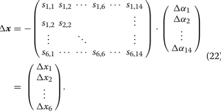
The detail form of Eq. (21) can be expressed as follows:

The input vector ∆Y is 1 × 1 order matrix, and the

coef-ficient matrix D is zero matrix, so Eq. (11) can be

simpli-fied as follows:

Define

(20)

�x= −



    

s1,1 s1,2 · · · s1,6 · · · s1,14

s1,2 s2,2 ... ..

. . .. ...

s6,1 · · · s6,6 · · · s6,14



    

·



  

�α1

�α₂ .. . �α14



  

−



  

s1,1 s2,1

.. .

s6,1 

  

·(�u1)=



  

�x1

�x2

.. . �x6



  

.

(21)

�x= −Sα·�α.

(22)

�x= −



    

s1,1 s1,2 · · · s1,6 · · · s1,14

s1,2 s2,2

. . . .

.

. . .. ...

s6,1 · · · s6,6 · · · s6,14



    

·



  

�α1

�α2 . . .

�α14



  

=



  

�x1

�x2 . . .

�x6



  

.

(23)

�Y =C·�x= −C·Sα·�α.

where SY_α is the PSM of output vector, D is coefficient

matrix, C is coefficient matrix.

Then, the output vector change can be expressed as follows:

Due to limited space, the detail expressions from Eqs.

(13) to (25) are not listed in this paper.

4 Sensitivity Analysis of HIVC 4.1 Dynamic Sensitivity Analysis 4.1.1 Orthogonal Test Design

Sinusoidal response can evaluate the tracing result with different frequency and amplitude, and its control result indicates the response performance and the control accu-racy, so the sinusoidal signal is chosen as the input signal to analyze the system parameter sensitivity of the HIVC force control system. Three working condition factors

including the system supply oil pressure Ps, the sinusoidal

frequency f and the sinusoidal amplitude A are chosen

and each factor has three levels. Ps are 6 MPa, 12 MPa,

and 18  MPa, f are 1  Hz, 2  Hz, and 4  Hz, A are 500  N,

1000  N and 1500  N. There should be 33 _{= 27 working}

conditions which will need superfluous work to complete the comprehensive test.

The orthogonal test design can make the comprehen-sive and superfluous test simplified to a few tests and

evaluate the comprehensive test [25, 26]. The orthogonal

test can be expressed as Ln(tc), where L is the orthogonal

test code, n is the test number and c is the number of the factors. In this paper, the orthogonal test of three factors

and three levels can be expressed as L9(34), which needs

nine tests to evaluate the comprehensive research, and

the detail orthogonal test table is shown in Table 3.

The range analysis table of orthogonal test is needed to evaluate the results of the comprehensive test after the results of these nine selected working conditions shown

in Table 3 are calculated. And the mean value of one level

within one factor can be expressed as follows:

where kβ is mean value of one factor and one level in

range analysis, subscript β shows the βth level within one

factor, subscript γ shows the γth result within this level

and l shows the number of level. Therefore, kβ can reflect

the proportion of this level in all levels, and the larger value indicates that this level within one factor can cause greater influence on result.

(24)

SY_α =C·Sα,

(25)

�Y = −SY_α ·�α.

(26) kβ =

l

γ=1

kβγ, Table 3 Nine working conditions selected by orthogonal

test design

No. System pressure Ps (MPa) Frequency f (Hz) Amplitude A (N)

1 6 1 500

2 6 2 1000

3 6 4 1500

4 12 1 1000

5 12 2 1500

6 12 4 500

7 18 1 1500

8 18 2 500

And the change range of one factor can be expressed as follows:

where R is range of one factor in range analysis. R can

reflect the change range of each level within one factor, and the larger value can reflect that the levels change within one factor can cause greater influence on the result.

(27)

R=max(kβ)−min(kβ),

4.1.2 Nine Working Conditions

To indicate each system parameter sensitivity charac-teristics, the force sinusoidal response simulation and experiment curves with two stable periods under the

nine selected working conditions are shown in Figure 5.

The amplitude attenuation and the phase lag are two typical performance indexes to evaluate the sinusoidal response and these two performance indexes under the

nine selected working conditions are shown in Table 4.

Time t/s

Sinusoidal response

N

/

F

Experimental curve Simulation curve Given displacement curve

0 0.4 0.8 1.2 1.6 2

T600 T400 T200 0 200 400 600

Time

Sinusoidal response

N

/

F

Experimental curve Simulation curve Given displacement curve

0 0.2 0.4 0.6 0.8 1

T1200

T900

T600

T3000 300 600 900 1200

t/s Time

Sinusoidal response

N_/

F

Experimental curve Simulation curve Given displacement curve

0 0.1 0.2 0.3 0.4 0.5

T1600

T1200

T800

T4000 400 800 1200 1600

t/s

Time

Sinusoidal response

N_/

F

Experimental curve Simulation curve Given displacement curve

0 0.4 0.8 1.2 1.6 2

T1200 T900

T600 T3000 300 600 900 1200

t/s Time

Sinusoidal response

N

/

F

Experimental curve Simulation curve Given displacement curve

0 0.2 0.4 0.6 0.8 1

T1600 T1200 T800 T4000 400 800 1200 1600

t/s Time

Sinusoidal response

N

/

F

Experimental curve Simulation curve Given displacement curve

0 0.1 0.2 0.3 0.4 0.5

T600

T400

T200 0 200 400 600

t/s

Time

Sinusoidal respons

e

N

/

F

Experimental curve Simulation curve Given displacement curve

0 0.4 0.8 1.2 1.6 2

T1600

T1200

T800

T4000 400 800 1200 1600

t/s Time

Sinusoidal response

N

/

F

Experimental curve Simulation curve Given displacement curve

0 0.2 0.4 0.6 0.8 1

T600 T400 T200 0 200 400 600

t/s Time

Sinusoidal response

N

/

F

Experimental curve Simulation curve Given displacement curve

0 0.1 0.2 0.3 0.4 0.5

T1200

T900

T600

T3000 300 600 900 1200

t/s

a

b

c

d

e

f

g

h

i

Table 4 Performance indexes under the nine selected working conditions

Performance index 1 2 3 4 5 6 7 8 9

Amplitude attenuation Φ (N)

Experiment 32.1 76.5 101.5 31.3 40.1 30.4 29.2 18.8 38.2

Simulation 9.5 41.7 185.9 12.1 31.2 18.6 14.2 6.1 27.1

Phase lag ψ (°)

Experiment 8.7 13.8 24.5 5.2 8.9 14.4 3.9 8.1 17.9

Simulation 5.0 10.5 20.8 3.5 7.1 13.2 2.8 5.4 10.8

As it can be seen in Table 4, the maximum

ampli-tude attenuation difference between the simulation and the experiment is about 5.6%, the maximum phase lag between the simulation and the experiment is 7.1°, and the maximum difference of the two performance indexes occurs when the sinusoidal frequency is 4 Hz. As the fre-quency is smaller, the difference of the two performance indexes between the simulation and the experiment are smaller. Moreover, when the working condition is 6 MPa, 4 Hz and 1500 N, the amplitude attenuation and phase lag differences between the simulation and the experi-ment are bigger than those under other working con-ditions, which is caused by that the maximum piston output force is about 1600 N when the system supply oil pressure is 6 MPa, and the bigger frequency can also lead the bigger values of the two performance indexes. Above all, the nine groups of simulation and experiment curves are fitting well respectively, which can indicate that the nonlinear mathematical model has relatively high accu-racy and its parameters setting is accurate.

Based on the orthogonal test, the simulation and exper-iment results of the two performance indexes under the nine selected working conditions can be used to derive the range analysis, and the range analysis table is shown

in Table 5, which can indicate the change rules of the

two performance indexes under the whole working conditions.

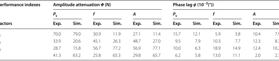
As it can be seen in Table 5, the two performance

indexes change rules of the simulation and experiment are the same. When the amplitude is bigger, the fre-quency is smaller or the supply oil pressure is smaller, the amplitude attenuation and the phase lag are bigger. Besides, the amplitude attenuation change range caused by these three factors change is similar, while the fre-quency change has the most effects on the phase lag and the amplitude change has the least effects on the phase lag.

4.1.3 PSM

For servo cylinder piston displacement, servo cylinder piston velocity, servo valve spool displacement, servo

valve spool velocity and two servo cylinder cavities pres-sure are equal to 0 at the initial moment, the initial

sys-tem state variable x is x0 =0. And PSM Sα are

where 0m×p is 6 × 14 order zero matrix. And the PSM of

output vector SY

α can be expressed as follows:

where the superscript 5 and 6 indicate the row number of

PSM related to the state variables x5 and x6 respectively.

The associated equations including Eqs. (13), (14), (16),

(18) and (29) are solved by programming on the

MAT-LAB. Then the PSM SY

α of each system parameter are

calculated under the nine selected working conditions,

and the time-history curves of PSM SY

α under the first

selected working condition which is 6 MPa, 1 Hz, 500 N

are shown in Figure 6.

As it can be seen in Figures 5(a) and 6, firstly, the PSM

change rules of parameter α1, α5, α7 and α14 are the same.

When the output force is zero as the piston speed is the

largest, the PSM of parameter α1, α5, α7 and α14 are zero,

and their change rules are sinusoidal. Secondly, the PSM of

parameter α2 is also zero when the output force is zero, but

its change rule is oppositely sinusoidal, which is different

from those of parameter α1, α5, α7 and α14. Thirdly, the PSM

change rules of parameter α4, α6, α8 and α10 are the same.

When the output force is zero, the PSM of parameter α4, α6,

α8 and α10 are the biggest and their change rules are

cosinoi-dal. Fourthly, The PSM change rules of the other parameter

α3, α9, α11, α12 and α13 are the same. When the output force

is zero, the PSM of parameter α3, α9, α11, α12 and α13 are the

biggest and their change rules are oppositely cosinoidal. Due to limited space, the PSM of the other eight work-ing conditions are not listed in this paper.

4.1.4 Time‑history Comparative Curves of Force Change

In order to indicate the influence of each parameter change on the sinusoidal force response characteristics of HIVC under the nine selected working conditions clearly,

the force output change ΔY can be expressed as

(28)

Sα0=0m×p,

(29)

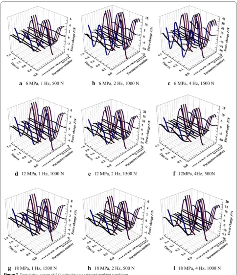
According to Eq. (30), the time-history curves of ∆Y are

shown in Figure 7, based on the PSM SY

α with parameter

increase 10% under the nine selected working conditions.

As it can be seen in Figure 7, the system parameters

increment can cause the output force change periodi-cally. In the following section, these dynamic changes are quantitatively analyzed to grasp the sensitivity change rule of each parameter under the nine selected working conditions.

4.2 Quantitative Sensitivity Analysis 4.2.1 Sensitivity Indexes

In this section, two measurable indexes of parameters sensitivity are defined to quantitatively analyze the char-acteristics of force change caused by the parameters change under the nine selected working conditions.

Denote the first measurable index of parameters

sensi-tivity s1 which is the mean valve of the amplitude

attenu-ation change after the parameters increase 10% in one stable period as follows:

where

where Φ1 is amplitude attenuation change caused by

the parameters change at the peak in one stable period,

Φ2 is amplitude attenuation change caused by the

parameters change at the trough in one stable period. Similarly,denote the second measurable index of

param-eters sensitivity s2 which is the mean valve of the phase

lag change after the parameters increase 10% in one sta-ble period as follows:

(30)

�Y = −SY_α ·�α_i.

(31)

s1=mean(Φ1+Φ2),

(32)

Φ1= [max(Fr)−max(F−SY_α ·�αi)] − [max(Fr)−max(F)]

=max(F₎−max(F−SY

α·�αi),

(33)

Φ2= [min(Fr)−min(F)] − [min(Fr)−min(F−SY_α·�αi)]

=min(F−SY

α·�αi)−min(F),

where ψ is phase lag change caused by the parameters

change in one stable period, as follows:

The influence degree of parameters change on piston

output force F can be evaluated quantitatively and clearly

by analyzing these two sensitivity indexes.

4.2.2 Sensitivity Indexes Histograms

According to Eqs. (31) and (34), the two sensitivity

indexes histograms are obtained to illustrate the sensi-tivity characteristics of each system parameter with each parameter increase 10% under the nine selected working

conditions. The histograms are shown in Figure 8.

As it can be seen in Figure 8, the sensitivity

character-istics of each parameter in HIVC under the nine selected working conditions are as below.

(1) The effects of each parameter increase 10% on the amplitude attenuation and phase lag are different under the same working condition. The two sen-sitivity indexes of parameters α4, α6, α7, α9 and α10

are quite smaller than those of the other parameters under the nine selected working conditions, indi-cating that the small fluctuation of the five param-eters has few effects on the HIVC force control performance. To research the main performance-influenced parameters selectively, the sensitivity of parameters α4, α6, α7, α9 and α10 is not detailedly

researched in this paper. And both α11 and α12 are

the forward path gains which have completely same sensitivity characteristics, so only the sensitivity characteristics of parameter α12 are analyzed in the

following sections. The effects of parameters α1, (34)

s2=mean(Ψ ),

(35)

Ψ =

arcsin

_F

r

max(F_r)

−arcsin

_F−SY α ·�αi

max(F₋SY

α ·�αi)

−

arcsin

_F

r

max(F_r)

−arcsin

_F

max(F₎

. Table 5 Range analysis table of two performance indexes

Performance indexes Amplitude attenuation Φ (N) Phase lag ψ (10‒2(°))

Ps f A Ps f A

Factors Exp. Sim. Exp. Sim. Exp. Sim. Exp. Sim. Exp. Sim. Exp. Sim.

k₁ 70.0 79.0 30.9 11.9 27.1 11.4 15.7 12.1 5.9 3.8 10.4 7.9

k₂ 33.9 20.6 45.1 26.3 48.7 27.0 9.5 7.9 10.3 7.7 12.3 8.3

k₃ 28.7 15.8 56.7 77.2 56.9 77.1 10.0 6.3 18.9 14.9 12.4 10.2

α2, α3, α5, α8, α12, α13 and α14 increase 10% on the

amplitude attenuation and phase lag are large and their sensitivity characteristics must be analyzed detailedly in the following.

(2) The parameters increase has positive or negative effects on the amplitude attenuation and phase lag. Taking sensitivity characteristics of α3, α12 and α13

as examples, the increasing of them can decrease

the amplitude attenuation and phase lag, which is caused by that the increasing of the system supply oil pressure α3 and control gain α12 will increase the

channel gain of the transfer function to enhance the system response speed and control accuracy. According to Figure 8, the parameters having posi-tive/negative effects on the system control perfor-mance should be enlarged/restrained to optimize

·) / ra d Ns ⋅

Sensitivity matrix Time t/s

3 10 − × (( )

0.0 0.4 0.8 1.2 1.6 2.0

T3 T2 T1 0 1 2 3 1 − N/ Sensitivity matrix Time t/s

0.0 0.4 0.8 1.2 1.6 2.0

T2 T1 0 1 2 Pa· (N ) / T 6 10 ×

Sensitivity matrix 0.0 0.4 0.8_{Time t/s}1.2 1.6 2.0

T4 T2 0 2 4 T 1 T 6 10 × / Pa· (N )

Sensitivity matrix 0.0 0.4 0.8Time t/s1.2 1.6 2.0

T6 T3 0 3 6 T 1

a

_b

2Y

S

c

_d

4Y S 13 10 × T 3 ·) (m Pas ⋅ ( ) /

Sensitivity matrix Time t/s

N

⋅

0.0 0.4 0.8 1.2 1.6 2.0

T4 T2 0 2 4 / Sensitivity matrix Time t/s m· (N )

0.0 0.4 0.8 1.2 1.6 2.0

T20 T10 0 10 20 T 1 / Sensitivity matrix

Time t/s

m·

(N

)

0.0 0.4 0.8 1.2 1.6 2.0

T1 0 1 2 T 1 _m N·( )

Sensitivity matrix _{Time t/s}

T

2

0.0 0.4 0.8 1.2 1.6 2.0

T15 T10 T5 0 5 10 15 10 × 4 /

e

_f

6

Y

S

g

_h

8Y S 10 × (N·Pa ) 10 − /

Sensitivity matrix 0.0 0.4 0.8Time t/s1.2 1.6 2.0

T15 T10 T5 0 5 10 15 T 1 kg N· ( / T 3 10 × ) Sensitivity matrix

Time t/s

0.0 0.4 0.8 1.2 1.6 2.0

T4 T2 0 2 4 T 1 5 10 × N / Sensitivity matrix

Time t/s

0.0 0.4 0.8 1.2 1.6 2.0

T6 T3 0 3 6 N / Sensitivity matrix

Time t/s

0.0 0.4 0.8 1.2 1.6 2.0

T6

T3 0 3 6

i

_j

10Y

S

k

_l

12Y S 5 10 − × m / / 4 10 − × · m s ) (

Sensitivity matrix Sensitivity matrix

Time t/s Time t/s 0.0 0.4 0.8 1.2 1.6 2.0

T10

T5 0 5 10

0.0 0.4 0.8 1.2 1.6 2.0

T₈ T₄ 0 4 8 T 1

the structure design and control strategy, which can improve the whole force control performance of HIVC. On the contrary, the secondary perfor-mance-influenced parameter whose fluctuation is small can be ignored.

(3) The amplitude attenuation and the phase lag can be used to evaluate the force control accuracy and response speed respectively, yet the two sensitiv-ity indexes plus-minus characteristics of some parameters are not the same. The two sensitivity indexes plus–minus characteristics of α1, α5 and α14

is opposite, when these three parameters increase, the amplitude attenuation increases and the phase lag decreases. The two performance indexes plus– minus characteristics of α8 is opposite under some

working conditions but the same under the other working conditions. Qualitatively speaking, the effective piston area of servo cylinder increasing enlarges the output force, which improves the sys-tem performance based on the force equilibrium equation, but the effective piston area of servo cyl-Parameters number

1 2 3 4 5 6 7 8 9 10 1112 1314 T1.5 T1 T0.5 0 0.5 1 1 S xe dni yti viti sn eS /N Parameters number 2 S xe dni yti viti sn eS (/° )

1 2 3 4 5 6 7 8 9 1011121314 T0.6 T0.3 0 0.3 0.6 Parameters number 1 2 3 4 5 6 7 8 9 10 11 12 13 14 T6 T3 0 3 1 S xe dni yti viti sn eS /N Parameters number 1 2 3 4 5 6 7 8 9 101112 13 14 T1 T0.5 0 0.5 1 2 S xe dni yti viti sn eS (/° )

a s1ands2with 6 MPa, 1 Hz, 500 N b s1ands2with 6 MPa, 2 Hz, 1000 N

Parameters number 1 2 3 4 5 6 7 8 9 1011121314 T30 T20 T10 0 10 1 S xe dni yti viti sn eS /N Parameters number 1 2 3 4 5 6 7 8 9 1011121314 T2 T1 0 1 2 2 S xe dni yti viti sn eS (/°) Parameters number 1 2 3 4 5 6 7 8 9 1011121314 T1.5 T1 T0.5 0 0.5 1 1 S xe dni yti viti sn eS /N Parameters number 1 2 3 4 5 6 7 8 9 1011121314 T0.4 T0.2 0 0.2 0.4 2 S xe dni yti viti sn eS (/° )

c s1ands2with 6 MPa, 4 Hz, 1500 N d s1ands2with 12 MPa, 1 Hz, 1000 N

Parameters number 1 2 3 4 5 6 7 8 9 1011121314 T4 T2 0 2 1 S xe dni yti viti_sn eS /N Parameters number 1 2 3 4 5 6 7 8 9 1011121314 T1 T0.5 0 0.5 1 2 S xe dni yti viti sn eS (/°) Parameters number 1 2 3 4 5 6 7 8 9 10 11 12 13 14 T4 T2 0 2 1 S xe dni yti viti sn eS /N Parameters number 1 2 3 4 5 6 7 8 9 1011121314 T2 T1 0 1 2 2 S xe dni yti viti sn eS (/° )

e s1ands2with 12 MPa, 2 Hz, 1500 N f s1ands2with 12 MPa, 4 Hz, 500 N

Parameters number

1 2 3 4 5 6 7 8 9 1011121314

T2 T1 0 1 2 1 S xe dni yti viti sn eS /N Parameters number 1 2 3 4 5 6 7 8 9 1011121314 T0.4 T0.2 0 0.2 0.4 2 S xe dni yti viti sn eS (/° ) Parameters number 1 2 3 4 5 6 7 8 9 1011121314 T1 T0.5 0 0.5 1 S xe dni yti viti sn eS /N Parameters number 1 2 3 4 5 6 7 8 9 10 11 12 13 14 T0.6 T0.3 0 0.3 0.6 2 S xe dni yti viti sn eS (/° )

g s1ands2with 18 MPa, 1 Hz, 1500 N h s1ands2with 18 MPa, 2 Hz, 500 N

Parameters number 1 2 3 4 5 6 7 8 9 10 11 12 13 14 T6 T3 0 3 6 1 S xe dni yti viti sn eS /N Parameters number 1 2 3 4 5 6 7 8 9 1011121314 T1 T0.5 0 0.5 1 2 S xe dni yti viti sn eS (/°)

i s1ands2with 18 MPa, 4 Hz, 1000 N

inder increasing enlarges the compressible oil vol-ume of the servo cylinder, which delays the pressure building time and has negative effects on the system performance. So the effect of it on the system per-formance is strongly related to the working condi-tions.

(4) As the working condition changes, the two sensitiv-ity indexes proportions of one parameter change, compared with those of the other parameters. The two sensitivity indexes proportions of α1, α3, α5, α8,

and α14 are large under some working conditions

but small under the other working condition, the compensation control are conducted to improve the HIVC force control performance.

(5) The two sensitivity indexes magnitude of different parameters is related to the magnitude of the ampli-tude attenuation and phase lag directly under one

working condition. In other words, when the mag-nitude of the amplitude attenuation and the phase lag is large or small, the magnitude of S1 and S2 is

large or small.

4.2.3 Range Analysis

In this section, according to the two sensitivity indexes histogram under the nine selected working conditions

shown in Figure 8, the two sensitivity indexes range

anal-ysis tables based on the orthogonal test theory are shown

in Table 6 and Table 7 respectively which can indicate the

change rules of sensitivity indexes to analyze the effects of each parameter on force control performance quan-titatively and the differences under different working conditions.

Table 6 Range analysis of each parameter S₁ (N)

Parameters ω ζ P_s C_ip

Factors Ps f A Ps f A Ps f A Ps f A

k₁ 1.5 0.2 0.5 − 1.6 − 0.2 − 0.5 − 10.7 − 0.9 − 0.9 1.4 1.0 0.5

k₂ 0.8 0.7 1.0 − 0.8 − 0.8 − 1.1 − 1.9 − 3.0 − 2.9 1.0 1.1 1.0

k₃ 0.8 2.2 1.6 − 0.8 − 2.2 − 1.6 − 1.3 − 10.1 − 10.1 0.8 1.0 1.6

R 0.7 2.0 1.1 0.8 2.0 1.1 9.4 9.2 9.2 0.6 0.1 1.1

Parameters Ap Kp K Bp

Factors Ps f A Ps f A Ps f A Ps f A

k₁ 0.7 − 0.6 0.6 − 8.5 − 1.3 − 1.5 − 8.7 − 0.5 − 1.5 1.9 0.2 0.5

k₂ 0.6 0.3 0.9 − 2.6 − 3.3 − 3.5 − 2.4 − 2.8 − 3.3 0.8 0.8 1.1

k₃ 0.6 2.4 0.5 − 2.1 − 8.6 − 8.2 − 2 − 9.7 − 8.3 0.8 2.5 1.9

R 0.1 3.0 0.4 6.4 7.3 6.7 6.7 9.2 6.8 1.1 2.3 1.4

Table 7 Range analysis of each parameter S₂ (10−2_(°))

Parameters ω ζ P_s C_ip

Factors Ps f A Ps f A Ps f A Ps f A

k₁ − 5.5 − 0.2 − 1.6 6.8 0.3 4.5 − 70.2 − 20.2 − 38.8 − 0.4 0.2 0.1

k₂ − 1.8 − 1.2 − 1.8 2.5 3.8 2.5 − 40.2 − 43.0 − 44.9 0.1 0.1 0.1

k₃ − 1.2 − 7.0 − 5.0 4.0 9.2 6.2 − 31.2 − 78.3 − 57.9 0.1 − 0.6 − 0.4

R 4.3 6.8 3.4 4.3 8.9 3.7 39.0 58.1 19.1 0.5 0.8 0.5

Parameters Ap Kp K Bp

Factors Ps f A Ps f A Ps f A Ps f A

k₁ 83.3 33.4 72.1 − 94.5 − 33.8 − 69.5 − 90.1 − 32.6 − 66.5 − 2.9 − 0.1 − 1.7 k₂ 70.2 63.6 69.8 − 69.5 − 66.8 − 71.9 − 66.5 − 64.5 − 69.0 − 1.6 − 0.5 − 1.3 k₃ 58.5 115.0 70.2 − 56.6 − 120.1 − 79.3 − 54.3 − 113.8 − 75.4 − 1.2 − 5 − 2.6

As it can be seen in Table 6 and Table 7, the sensitivity change rules of each parameter in HIVC under the whole working conditions are below:

Firstly, the mean value of one level within one factor

kβ can indicate that the change rules of the effects that

each factor has on the two sensitivity indexes of

param-eters α1, α2, α3, α12, α13 and α14 are quite similar to the

change rules of the amplitude attenuation and phase lag

shown in Table 5 under the whole working conditions.

Frequency f has small effects on S1 of α5, and each

fac-tor change has effects on the plus–minus characteristic

of its S2. In addition, the effects of each parameter on S1

of α8 are different from those of the other parameters,

and even the plus-minus characteristics of its S1 can be

changed with the frequency f change, yet the frequency f

has few effects on its S2.

Secondly, the change range of one factor R can indicate

that the frequency f is the main factor influencing S1 of

α1, α2, α8, α13 and α14. And the amplitude A is the main

factor influencing S1 of α5. Moreover, each factor of α3

and α11 has similar effects on S1. While the frequency f

is the main factor influencing S2 of all the parameters,

which can indicate that frequency f has great effects on

the phase lag.

5 Experiments

Due to the limited experimental conditions and the immeasurable parameters, lots of parameters in force control system of HIVC can’t be measured directly so that their sensitivity characteristics can’t be verified experimentally. However, all parameters sensitivity anal-ysis is based on the same force control mathematical model and the sensitivity mathematical model, the anal-ogy method can be used to deduce some immeasurable parameters sensitivity characteristics from experimental verification of some measurable parameters sensitivity characteristics.

System supply oil pressure α3, initial piston

posi-tion of servo cylinder α7 and proportional gain α12 can

be measured online, so their sensitivity characteristics can be verified experimentally. The initial output force is subtracted from the final output force caused by the parameters increasing. Moreover, the multiple-sampling average method is adopted to ensure the experimental results accuracy. And the comparative histograms of two sensitivity indexes with parameters increase 10% under the nine selected working conditions are shown from

Figure 9.

As it can be seen in Figure 9, the two sensitivity indexes

experimental results of L0 are quite small, which can

ver-ify the theoretical results of them. Therefore, the effects

of L0 on the force control performance can be ignored

when it has relatively small fluctuation, and the detail results of it are not analyzed in this section. Moreover,

the two sensitivity indexes experimental results of Ps and

Kp are quite close to the theoretical results, and the detail

range and error analysis of their sensitivity indexes under

the whole working conditions are shown in Table 8 and

Table 9, in which errors of S1 and S2 are both equal to the

absolute value of the difference between the experiment and the simulation values.

As it can be seen in Table 8 and Table 9, the two

sen-sitivity indexes differences of Ps and Kp between

experi-mental results and theoretical results are small under the

whole working conditions. For Ps, its S1 maximum

differ-ences of kβ and R are 1.7 and 1.9, respectively, and its S2

maximum differences of kβ and R are 0.092° and 0.121°,

respectively. For Kp, its S1 maximum differences of kβ and

R are 1.2 and 1.6, respectively, and its S2 maximum

dif-ferences of kβ and R are 0.092° and 0.121°, respectively.

Furthermore, the large differences are usually generated

when the Ps is small and the f and A are large.

The reason why the differences exist is that the force control system mathematical model of HIVC whose accuracy influences each system parameter sensitivity

1 2 3 4 5 6 7 8 9 T30

T20 T10 0

Experiment Theory

Number of working conditions

1

S

xe

dni

yti

viti

sn

eS

/N

2

S

xe

dni

yti

viti

sn

eS

(/°

)

Experiment Theory

Number of working conditions 1 2 3 4 5 6 7 8 9 T1.5

T1 T0.5 0

a System pressurePs

1

S

xe

dni

yti

viti_sn

eS

/N

Number of working conditions 1 2 3 4 5 6 7 8 9

0 0.002 0.004 0.006 0.008

0.01 Theory_Experiment

2

S

xe

dni

yti

viti

sn_eS

(/°)

Experiment Theory

Number of working conditions 1 2 3 4 5 6 7 8 9 T1.2

T0.8 T0.4 0

x

10

-3

b Initial piston position of servo cylinderL0

Experiment Theory

Number of working conditions 1 2 3 4 5 6 7 8 9 T20

T15 T10 T5 0

1

S

xe

dni

yti

viti

sn

eS

/N

Experiment Theory

Number of working conditions 1 2 3 4 5 6 7 8 9 T1.5

T1 T0.5 0

2

S

xe

dni

yti

viti

sn

eS

(/°

)

c Proportional gainKp

analysis results can’t accurately describe all the practi-cal system characteristics, so the differences between the simulation results and experiment results are inevitable.

6 Conclusions

(1) The PSM of each parameter and the dynamic fig-ures of the output force change with each param-eter increase 10% can indicate that each paramparam-eter change has different dynamic effects on the sinusoi-dal output force and each parameter PSM changes periodically including sinusoid, opposite sinusoid, cosine and opposite cosine whose ranges are differ-ent and change with differdiffer-ent working conditions. (2) The two sensitivity indexes are built to evaluate

the effects of each parameter increase 10% on the amplitude attenuation and the phase lag of the sinusoidal output force response. The results can indicate that system parameters increasing have positive or negative effects on the two sensitivity indexes. Moreover, the range analysis can indicate that the two sensitivity indexes of each parameter change with different working conditions including three working conditions factor.

(3) The two sensitivity indexes of the system return oil pressure, the total piston stroke of servo cylinder,the initial piston position of servo cylinder, the effective bulk modulus and the conversion mass are small under the nine selected working conditions. While the two sensitivity indexes of the natural frequency of servo valve, the damping ratio of servo valve,

Table 8 Range and error analysis table of P_s sensitivity indexes

Sensitivity indexes S1 (N) S2 (10−2 (°))

Factors Ps f A Ps f A

Exp. Sim. Err. Exp. Sim. Err. Exp. Sim. Err. Exp. Sim. Err. Exp. Sim. Err. Exp. Sim. Err.

k₁ − 9.5 − 10.7 1.2 − 1.1 − 0.9 0.2 − 1.0 − 0.9 0.1 − 66.3 − 70.2 3.9 − 21.2 − 20.2 1.0 − 41.0 − 38.8 3.2 k₂ − 2.2 − 1.9 0.3 − 3.5 − 3.0 0.5 − 3.2 − 2.9 0.3 − 40.8 − 40.2 0.6 − 44.1 − 43.0 1.1 − 50.3 − 44.9 5.4 k₃ − 1.3 − 1.3 0 − 8.4 − 10.1 1.7 − 8.7 − 10.1 1.4 − 34.5 − 31.2 3.3 − 76.5 − 78.3 1.8 − 48.7 − 57.9 9.2

R 8.2 9.4 1.2 7.3 9.2 1.9 7.7 9.2 1.5 31.8 39.0 7.2 55.3 58.1 2.8 7.7 19.1 12.1

Table 9 Range analysis table of K_p sensitivity indexes

Sensitivity indexes S1 (N) S2 (10−2 (°))

Ps f A Ps f A

Factors Exp. Sim. Err. Exp. Sim. Err. Exp. Sim. Err. Exp. Sim. Err. Exp. Sim. Err. Exp. Sim. Err.

k₁ − 7.5 −8.5 1.0 − 1.5 − 1.3 0.2 − 1.9 − 1.5 0.4 − 92.1 − 94.5 2.4 − 41.7 − 33.8 7.9 − 71.8 − 69.5 2.3 k₂ − 2.7 − 2.6 0.1 − 3.7 − 3.3 0.4 − 4.0 − 3.5 0.5 − 70.5 − 69.5 1.0 − 75.4 − 66.8 8.6 − 74.8 − 71.9 2.9 k₃ − 2.6 − 2.1 0.5 − 7.8 − 8.6 0.8 − 7.0 − 8.2 1.2 − 57.9 − 56.6 1.3 − 105.8 − 120.1 14.3 − 75.4 − 79.3 3.9

R 4.9 6.4 1.5 6.3 7.3 1.0 5.1 6.7 1.6 34.2 37.9 3.7 64.1 86.3 22.2 3.6 9.8 6.2

the system supply oil pressure, the internal leakage coefficient, the effective piston area of servo cylin-der, the proportional gain, the force sensor gain and the viscous damping coefficient are large.

Authors’ Contributions

X‑DK and L‑JK were in charge of the whole trial; K‑XB and BY wrote the manu‑ script; H‑LZ, Q‑XZ and C‑HL assisted with sampling and laboratory analyses. All authors read and approved the final manuscript.

Author details

1 _{School of Mechanical Engineering, Yanshan University, Qinhuangdao 066004,} China. 2 _{State Key Laboratory of Fluid Power and Mechatronic System,} Zhejiang University, Hangzhou 310027, China. 3 _{Columbia University, New} York 10027, USA.

Authors’ Information

Kai‑Xian Ba, born in 1989, is currently a PhD candidate at Yanshan University, China. His research interest is electro‑hydraulic servo control system. Tel: +86‑ 18630472204; E‑mail: bkx@ysu.edu.cn.

Bin Yu, born in 1985, is currently a lecture at Yanshan University, China. His research interest is fluid transmission and robot control. Tel: +86‑ 13930342639; E‑mail: yb@ysu.edu.cn.

Xiang‑Dong Kong, born in 1959, is currently a professor at Yanshan Univer‑ sity, China. He received his PhD degree from Yanshan University, China, in 1991. His main research interests include electro‑hydraulic servo control system and robot control theory. Tel: +86‑335‑8051166; E‑mail: xdkong@ysu.edu.cn.

Chun‑He Li, born in 1989, is currently a master candidate at Yanshan Uni‑ versity, China. His research interest is modeling in servo control system. E‑mail: 345082951@qq.com.

Qi‑Xin Zhu, born in 1992, is currently a master candidate at Yanshan Uni‑ versity, China. His research interest is valve−controlled cylinder force control system. E‑mail: 1755228049@qq.com.

Hua‑Long Zhao, born in 1993, is currently a master candidate at Yanshan University, China. His research interest is robot control and modeling. E‑mail: 731515432@qq.com.