Attention Based Spatial-Temporal Graph Convolutional Networks for Traffic Flow Forecasting

The Thirty-Third AAAI Conference on Artificial Intelligence (AAAI-19)

Attention Based Spatial-Temporal Graph Convolutional Networks

for Traffic Flow Forecasting

Shengnan Guo,

Youfang Lin,

Ning Feng,

Chao Song,

Huaiyu Wan

2_{Beijing Key Laboratory of Traffic Data Analysis and Mining, Beijing, China} 3_{CAAC Key Laboratory of Intelligent Passenger Service of Civil Aviation, Beijing, China}

{guoshn, yflin, fengning, chaosong, hywan}@bjtu.edu.cn

Abstract

Forecasting the traffic flows is a critical issue for researchers and practitioners in the field of transportation. However, it is very challenging since the traffic flows usually show high nonlinearities and complex patterns. Most existing traffic flow prediction methods, lacking abilities of modeling the dy-namic spatial-temporal correlations of traffic data, thus can-not yield satisfactory prediction results. In this paper, we propose a novel attention based spatial-temporal graph con-volutional network (ASTGCN) model to solve traffic flow forecasting problem. ASTGCN mainly consists of three in-dependent components to respectively model three tempo-ral properties of traffic flows, i.e., recent, daily-periodic and weekly-periodic dependencies. More specifically, each com-ponent contains two major parts: 1) the spatial-temporal at-tention mechanism to effectively capture the dynamic spatial-temporal correlations in traffic data; 2) the spatial-spatial-temporal convolution which simultaneously employs graph convolu-tions to capture the spatial patterns and common standard convolutions to describe the temporal features. The output of the three components are weighted fused to generate the fi-nal prediction results. Experiments on two real-world datasets from the Caltrans Performance Measurement System (PeMS) demonstrate that the proposed ASTGCN model outperforms the state-of-the-art baselines.

Introduction

Recently, many countries are committed to vigorously de-velop the Intelligent Transportation System (ITS) (Zhang et al. 2011) to help for efficient traffic management. Traf-fic forecasting is an indispensable part of ITS, especially on the highway which has large traffic flows and fast driving speed. Since the highway is relatively closed, once a conges-tion occurs, it will seriously affect the traffic capacity. Traf-fic flow is a fundamental measurement reflecting the state of the highway. If it can be predicted accurately in advance, ac-cording to this, traffic management authorities will be able to guide vehicles more reasonably to enhance the running efficiency of the highway network.

Highway traffic flow forecasting is a typical problem of spatial-temporal data forecasting. Traffic data are recorded at fixed points in time and at fixed locations distributed

∗

Corresponding author: [email protected]

Copyright c⃝2019, Association for the Advancement of Artificial Intelligence (www.aaai.org). All rights reserved.

9:00 AM 5:00 PM

A B

C

D

(a) Spatial influence of traffic flows at different times

(b) Temporal influence between traffic flows

0 t-4 t-2 t-1 t t+1 t+2 time

flow

history forecast

t-3 A

B

In

fl

u

en

ce

1

0 A

B

C

D

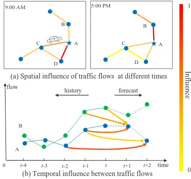
Figure 1: The spatial-temporal correlation diagram of traffic flow

in continuous space. Apparently, the observations made at neighboring locations and time stamps are not independent but dynamically correlated with each other. Therefore, the key to solve such problems is to effectively extracting the spatial-temporal correlations of data. Fig. 1 demonstrates the spatial-temporal correlations of traffic flows (also can be ve-hicle speed, lane occupancy, etc.). The bold line between two points represents their mutual influence strength. The darker the color of line is, the greater the influence is. In the spatial dimension (Fig. 1(a)), we can find that different loca-tions have different impacts on A and even a same location has varying influence on A as time goes by. In the temporal dimension (Fig. 1(b)), the historical observations of differ-ent locations have varying impacts on A’s traffic states at different times in the future. In conclusion, the correlations in traffic data on the highway network show strong dynamics in both the spatial dimension and temporal dimension. How to explore nonlinear and complex spatial-temporal data to discover its inherent spatial-temporal patterns and to make accurate traffic flow predictions is a very challenging issue.

device is placed at a unique geospatial location, constantly generating time series data about traffic. These devices have accumulated a large amount of rich traffic time series data with geographic information, providing a solid data founda-tion for traffic forecasting. Many researchers have already made great efforts to solve such problems. Early, time series analysis models are employed for traffic prediction prob-lems. Yet, it is difficult for them to handle the unstable and nonlinear data in practice. Later, traditional machine learn-ing methods are developed to model more complex data, but it is still difficult for them to simultaneously consider the spatial-temporal correlations of high-dimensional traffic data. Moreover, the prediction performances of this kind of methods rely heavily on feature engineering, which often re-quires lots of experiences from experts in the corresponding domain. In recent years, many researchers use deep learn-ing methods to deal with high-dimensional spatial-temporal data, i.e., convolutional neural networks (CNN) are adopted to effectively extract the spatial features of grid-based data; graph convolutional neural networks (GCN) are used for de-scribing spatial correlation of graph-based data. However, these methods still fail to simultaneously model the spatial-temporal features and dynamic correlations of traffic data.

In order to tackle the above challenges, we pro-pose a novel deep learning model: Attention based

Spatial-TemporalGraphConvolutionNetwork(ASTGCN) to collectively predict traffic flow at every location on the traffic network. This model can process the traffic data di-rectly on the original graph-based traffic network and ef-fectively capture the dynamic spatial-temporal features. The main contributions of this paper are summarized as follows:

• We develop a spatial-temporal attention mechanism to learn the dynamic spatial-temporal correlations of traffic data. Specifically, a spatial attention is applied to model the complex spatial correlations between different loca-tions. A temporal attention is applied to capture the dy-namic temporal correlations between different times.

• A novel spatial-temporal convolution module is designed for modeling spatial-temporal dependencies of traffic data. It consists of graph convolutions for capturing spa-tial features from the original graph-based traffic network structure and convolutions in the temporal dimension for describing dependencies from nearby time slices.

• Extensive experiments are carried out on real-world high-way traffic datasets, which verify that our model achieves the best prediction performances compared to the existing baselines.

Related work

Traffic forecasting After years of continuous researches and practices, many achievements have been made in the studies about traffic forecasting. The statistical models used for traffic prediction include HA, ARIMA (Williams and Hoel 2003), VAR (Zivot and Wang 2006), etc. These ap-proaches require data to satisfy some assumptions, but traf-fic data is too complex to satisfy these assumptions, so they usually perform poorly in practice. Machine learning meth-ods such as KNN (Van Lint and Van Hinsbergen 2012) and

SVM (Jeong et al. 2013) can model more complex data, but they need careful feature engineering. Since deep learning has brought about breakthroughs in many domains, such as speech recognition and image processing, more and more researchers apply deep learning to spatial-temporal data pre-diction. Zhang et al. (2018) designed a ST-ResNet model based on the residual convolution unit to predict crowd flows. Yao et al. (2018b) proposed a method to predict traffic by integrating CNN and long-short term memory (LSTM) to jointly model both spatial and temporal dependencies. Yao et al. (2018a) further proposed a Spatial-Temporal Dynamic Network for taxi demand prediction which can learn the sim-ilarity between locations dynamically. Although the spatial-temporal features of the traffic data can be extracted by these model, their limitation is that the input must be standard 2D or 3D grid data.

Convolutions on graphs The traditional convolution can effectively extract the local patterns of data, but it can only be applied for the standard grid data. Recently, the graph convolution generalizes the traditional convolution to data of graph structures. Two mainstreams of graph convolution methods are the spatial methods and the spectral methods. The spatial methods directly perform convolution filters on a graph’s nodes and their neighbors. So, the core of this kind of methods is to select the neighborhood of nodes. Niepert, Ahmed, and Kutzkov (2016) proposed a heuristic linear method to select the neighborhood of every center node, which achieved good results in social network tasks. Li et al. (2018) introduced graph convolutions into human action recognition tasks. Several partitioning strategies were proposed here to divide the neighborhood of each node into different subsets and to ensure the numbers of each node’s subsets are equal. The spectral methods, in which the lo-cality of the graph convolution is considered by spectral analysis. A general graph convolution framework based on the Graph Laplacian is proposed by Bruna et al. (2014), then Defferrard, Bresson, and Vandergheynst (2016) opti-mized the method by using Chebyshev polynomial approx-imation to realize eigenvalue decomposition. Yu, Yin, and Zhu (2018) proposed a gated graph convolution network for traffic prediction based on this method, but the model does not consider the dynamic spatial-temporal correlations of traffic data.

to be trained for each time series.

Motivated by the studies mentioned above, considering the graph structure of the traffic network and the dynamic spatio-temporal patterns of the traffic data, we simultane-ously employ graph convolutions and the attention mecha-nisms to model the network-structure traffic data.

Preliminaries

Traffic Networks

In this study, we define a traffic network as an undirected graphG= (V, E,A), as shown in Fig. 2(a), whereV is a finite set of|V|=N nodes;E is a set of edges, indicating the connectivity between the nodes; A ∈ RN×N denotes

the adjacency matrix of graphG. Each node on the traffic networkGdetectsFmeasurements with the same sampling frequency, that is, each node generates a feature vector of lengthF at each time slice, as shown by the solid lines in Fig. 2(b).

(b) 1

𝑡𝑖𝑚𝑒 flow occupy speed forecasting target

(a)

0 𝑡𝑖𝑚𝑒

Figure 2: (a) The spatial-temporal structure of traffic data, where the data at each time slice forms a graph; (b) Three measurements are detected on a node and the future traf-fic flow is the forecasting target. Here, all measurements are normalized to [0,1].

Traffic Flow Forecasting

Suppose thef-th time series recorded on each node in the traffic network G is the traffic flow sequence, and f ∈

(1, ..., F). We use xc,i_t ∈ R to denote the value of the c-th feature of node i at time t , and xit ∈ RF denotes

the values of all the features of node i at time t. Xt = (x1

t,x2t, ...,xtN)T ∈RN×F denotes the values of all the

fea-tures of all the nodes at timet.X = (X1,X2, ...,Xτ)T ∈ RN×F×τdenotes the value of all the features of all the nodes

overτtime slices. In addition, we setyti=x f,i

t ∈Rto

rep-resent the traffic flow of nodeiat timetin the future.

Problem. Given X, all kinds of the historical measure-ments of all the nodes on the traffic network over past

τ time slices, predict future traffic flow sequences Y = (y1_,y2_{, ...,y}N₎T _∈

RN×Tp of all the nodes on the whole

traffic network over the next Tp time slices, where yi = (yi

τ+1, yiτ+2, ..., yτi+Tp) ∈ R

Tp _{denotes the future traffic}

flow of nodeifromτ+ 1.

Attention Based Spatial-Temporal Graph

Convolutional Networks

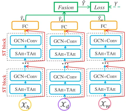
Fig. 3 presents the overall framework of the ASTGCN model proposed in this paper. It consists of three indepen-dent components with the same structure, which are de-signed to respectively model the recent, daily-periodic and weekly-periodic dependencies of the historical data.

Fusion 𝑌෠ 𝑌

FC FC FC

Loss

S

T bloc

k

S

T bloc

k

𝒳

𝒳

𝒳

SAtt+TAtt GCN+Conv

…

SAtt+TAtt GCN+Conv

…

SAtt+TAtt GCN+Conv

…

෠

𝑌𝑑 𝑌෠𝑤

෠

𝑌ℎ

Figure 3: The framework of ASTGCN. SAtt: Spatial Atten-tion; TAtt: Temporal Attention GCN: Graph ConvoluAtten-tion; Conv: Convolution; FC: Fully-connected; ST block: Spatial-Temporal block.

Suppose the sampling frequency isq times per day. As-sume that the current time ist0 and the size of predicting

window isTp. As shown in Fig. 4, we intercept three time series segments of lengthTh,TdandTwalong the time axis

as the input of the recent, daily-period and weekly-period component respectively, whereTh,TdandTware all integer

multiples ofTp. Details about the three time series segments are as follows:

(1) Therecentsegment:

Xh= (Xt0−Th+1,Xt0−Th+2, ...,Xt0)∈R

N×F×Th_{, a}

seg-ment of historical time series directly adjacent to the predict-ing period, as shown by the green part of Fig. 4. Intuitively, the formation and dispersion of traffic congestions are grad-ual. So, the just past traffic flows inevitably have influence on the future traffic flows.

(2) Thedaily-periodicsegment:

Xd= (Xt0−(Td/Tp)∗q+1, ...,Xt0−(Td/Tp)∗q+Tp,

Xt0−(Td/Tp−1)∗q+1, ...,Xt0−(Td/Tp−1)∗q+Tp, ...,

Xt0−q+1, ...,Xt0−q+Tp) ∈ R

N×F×Td _{consists of the}

seg-ments on the past few days at the same time period as the predicting period, as shown by the red part of Fig. 4. Due to the regular daily routine of people, traffic data may show repeated patterns, such as the daily morning peaks. The pur-pose of the daily-period component is to model the daily periodicity of traffic data.

(3) Theweekly-periodicsegment:

Xt0−7∗(Tw/Tp−1)∗q+1, ...,Xt0−7∗(Tw/Tp−1)∗q+Tp, ...,

Xt0−7∗q+1, ...,Xt0−7∗q+Tp) ∈ R

F×N×Tw _{is composed of}

the segments on last few weeks, which have the same week attributes and time intervals as the forecasting period, as shown by the blue part of Fig. 4. Usually, the traffic patterns on Monday have a certain similarity with the traffic patterns on Mondays in history, but may be greatly different from those on weekends. Thus, the weekly-period component is designed to capture the weekly periodic features in traffic data.

6/14/2018 Thur. 8:00-8:55 am

6/14/2018 Thur. 6:00-7:55 am

𝑇ℎ

… …

6/13/2018 Wed. 8:00-8:55 am 6/12/2018 Tue.

8:00-8:55 am 𝑇𝑑

… …

6/17/2018 Thur. 8:00-8:55 am 5/31/2018 Thur.

8:00-8:55 am

… …

𝑇𝑤

𝑇𝑝

Figure 4: An example of constructing the input of time series segments (suppose the size of predicting window is 1 hour, andTh,TdandTware twice ofTp.

The three components share the same network structure and each of them consists of several spatial-temporal blocks and a fully-connected layer. There are a spatial-temporal at-tention module and a spatial-temporal convolution module in each spatial-temporal block. In order to optimize the train-ing efficiency, we adopted a residual learntrain-ing framework (He et al. 2016) in each component. In the end, the out-puts of the three components are further merged based on a parameter matrix to obtain the final prediction result. The overall network structure is elaborately designed to describe the dynamic spatial-temporal correlations of traffic flows.

Spatial-Temporal Attention

A novel spatial-temporal attention mechanism is proposed in our model to capture the dynamic spatial and temporal correlations on the traffic network (as described in Fig. 1). It contains two kinds of attentions, i.e., spatial attention and temporal attention.

Spatial attention In the spatial dimension, the traffic con-ditions of different locations have influence among each other and the mutual influence is highly dynamic. Here, we use an attention mechanism (Feng et al. 2017) to adaptively capture the dynamic correlations between nodes in the spa-tial dimension.

Take the spatial attention in the recent component as an example:

S=Vs·σ((X (r−1)

h W1)W2(W3X (r−1)

h )

T _+b s) (1)

S′_i,j = exp(Si,j)

∑N

j=1exp(Si,j)

(2)

whereX(_hr−1) = (X1,X2, ...XTr−1) ∈ R

N×Cr−1×Tr−1 _is

the input of therth_{spatial-temporal block.Cr}

−1is the

num-ber of channels of the input data in the rth _{layer. When} r= 1,C0=F.Tr−1is the length of the temporal

dimen-sion in therth_{layer. Whenr= 1, in the recent component} T0 = Th(in the daily-period component T0 = Td and in

the weekly-period componentT0 =Tw).Vs,bs ∈RN×N,

W1 ∈ RTr−1_,W

2 ∈RCr−1×Tr−1_,W

3 ∈ RCr−1 _are learn-able parameters and sigmoid σ is used as the activation function. The attention matrixS is dynamically computed according to the current input of this layer. The value of an elementSi,jinSsemantically represents the correlation

strength between nodeiand nodej. Then a softmax func-tion is used to ensure the attenfunc-tion weights of a node sum to one. When performing the graph convolutions, we will ac-company the adjacency matrixAwith the spatial attention matrixS′∈RN×N to dynamic adjust the impacting weights

between nodes.

Temporal attention In the temporal dimension, there ex-ist correlations between the traffic conditions in different time slices, and the correlations are also varying under dif-ferent situations. Likewise, we use an attention mechanism to adaptively attach different importance to data:

E=Ve·σ(((X (r−1)

h )

T

U1)U2(U3X (r−1)

h ) +be) (3)

E′i,j=

exp(Ei,j)

∑Tr−1

j=1 exp(Ei,j)

(4)

whereVe,be ∈ RTr−1×Tr−1_,U

1 ∈ RN,U2 ∈ RCr−1×N_,

U3 ∈ RCr−1 are learnable parameters. The temporal

cor-relation matrixEis determined by the varying inputs. The value of an element Ei,j in E semantically indicates the

strength of dependencies between timeiandj. At last,Eis normalized by the softmax function. We directly apply the normalized temporal attention matrix to the input and get

ˆ

X(hr−1) = ( ˆX1,Xˆ2, ...,XˆTr−1) = (X1,X2, ...,XTr−1)E ′ _∈

RN×Cr−1×Tr−1_{to dynamically adjust the input by merging} relevant information.

Spatial-Temporal Convolution

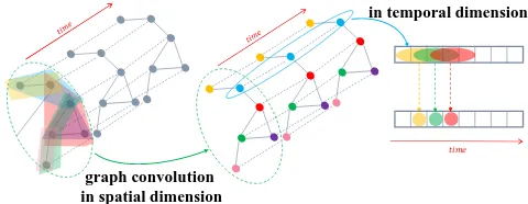
The spatial-temporal attention module let the network auto-matically pay relatively more attention on valuable informa-tion. The input adjusted by the attention mechanism is fed into the spatial-temporal convolution module, whose struc-ture is presented in Fig. 5. The spatial-temporal convolution module proposed here consists of a graph convolution in the spatial dimension, capturing spatial dependencies from neighborhood and a convolution along the temporal dimen-sion, exploiting temporal dependencies from nearby times.

𝑡𝑖𝑚𝑒

graph convolution in spatial dimension

convolution in temporal dimension

Graph convolution in spatial dimension The spectral graph theory generalizes the convolution operation from grid-based data to graph structure data. In this study, the traffic network is a graph structure in nature, and the fea-tures of each node can be regarded as the signals on the graph (Shuman et al. 2013). Hence, in order to make full use of the topological properties of the traffic network, at each time slice we adopt graph convolutions based on the spectral graph theory to directly process the signals, exploit-ing signal correlations on the traffic network in the spatial dimension. The spectral method transforms a graph into an algebraic form to analyze the topological attributes of graph, such as the connectivity in the graph structure.

In spectral graph analysis, a graph is represented by its corresponding Laplacian matrix. The properties of the graph structure can be obtained by analyzing Laplacian matrix and its eigenvalues. Laplacian matrix of a graph is defined as L = D−A, and its normalized form is L = IN −

D−12_AD−12 ∈ _RN×N_{, whereAis the adjacent matrix, IN} is a unit matrix, and the degree matrixD∈ RN×N is a

di-agonal matrix, consisting of node degrees,Dii = ∑jAij.

The eigenvalue decomposition of the Laplacian matrix is L = UΛUT, whereΛ = diag([λ0, ..., λN−1]) ∈ RN×N

is a diagonal matrix, andUis Fourier basis. Taking the traf-fic flow at timetas an example, the signal all over the graph isx=xf_t ∈_RN_{, and the graph Fourier transform of the}

sig-nal is defined asxˆ = UTx. According to the properties of the Laplacian matrix,Uis an orthogonal matrix, so the cor-responding inverse Fourier transform isx=Uxˆ. The graph convolution is a convolution operation implemented by us-ing linear operators that diagonalize in the Fourier domain to replace the classical convolution operator (Henaff, Bruna, and LeCun 2015). Based on this, the signalxon the graph

Gis filtered by a kernelgθ:

gθ∗Gx=gθ(L)x=gθ(UΛUT)x=Ugθ(Λ)UTx (5)

where ∗G denotes a graph convolution operation. Since

the convolution operation of the graph signal is equal to the product of these signals which have been transformed into the spectral domain by graph Fourier transform (Si-monovsky and Komodakis 2017), the above formula can be understood as Fourier transforming gθ and xrespectively

into the spectral domain, then multiplying their transformed results, and doing the inverse Fourier transform to get the final result of the convolution operation. However, it is ex-pensive to directly perform the eigenvalue decomposition on the Laplacian matrix when the scale of the graph is large. Therefore, Chebyshev polynomials are adopted in this pa-per to solve this problem approximately but efficiently (Si-monovsky and Komodakis 2017):

gθ∗Gx=gθ(L)x= K−1

∑

k=0

θkTk(˜L)x (6)

where the parameterθ∈ RKis a vector of polynomial

co-efficients.L˜ = _λ2

maxL−IN,λmaxis the maximum

eigen-value of the Laplacian matrix. The recursive definition of the Chebyshev polynomial isTk(x) = 2xTk−1(x)−Tk−2(x),

whereT0(x) = 1,T1(x) = x. Using approximate expan-sion of Chebyshev polynomial to solve this formulation cor-responds to extracting information of the surrounding 0 to

(K −1)th_{-order neighbors centered on each node in the}

graph by the convolution kernelgθ. The graph convolution

module uses the Rectified Linear Unit (ReLU) as the final activation function, i.e., ReLU(gθ∗Gx).

In order to dynamically adjust the correlations between nodes, for each term of Chebyshev polynomial, we accom-panyTk(L˜)with the spatial attention matrixS

′

∈ RN×N,

then obtainTk(L˜)⊙S′, where⊙is the Hadamard product.

Therefore, the above graph convolution formula changes to

gθ∗Gx=gθ(L)x=∑K_k=0−1θk(Tk(˜L)⊙S′)x.

We can generalize this definition to the graph signal with multiple channels. For example, in the recent

com-ponent, the input is Xˆ(_hr−1) = ( ˆX1,Xˆ2, ...,XˆTr−1) ∈

RN×Cr−1×Tr−1 , where the feature of each node hasCr−1

channels. For each time slicet, performingCrfilters on the graphXˆt, we getgθ∗GXˆt, whereΘ = (Θ1,Θ2, ...,ΘCr)∈

RK×Cr−1×Cr_{is the convolution kernel parameter (Kipf and}

Welling 2017). Therefore, each node is updated by the infor-mation of the 0∼K-1 neighbors of the node.

Convolution in temporal dimension After the graph con-volution operations having captured neighboring informa-tion for each node on the graph in the spatial dimension, a standard convolution layer in the temporal dimension is fur-ther stacked to update the signal of a node by merging the information at the neighboring time slice, as shown by the right part in Fig. 5. Also take the operation on therth_layer

in the recent component as an example:

X(_hr)=ReLU(Φ∗(ReLU(gθ∗GXˆ (r−1)

h )))∈R

Cr×N×Tr

(7) where∗denotes a standard convolution operation,Φis the parameters of the temporal dimension convolution kernel, and the activation function is ReLU.

In conclusion, a spatial-temporal convolution module is able to well capture the temporal and spatial features of traffic data. A spatial-temporal attention module and a temporal convolution module forms a spatial-temporal block. Multiple spatial-spatial-temporal blocks are stacked to further extract larger range of dynamic spatial-temporal correlations. Finally, a fully connected layer is appended to make sure the output of each component has the same dimension and shape with the forecasting target. The final fully connected layer uses ReLU as the activation function.

Multi-Component Fusion

the outputs of different components are fused, the impacting weights of the three components for each node are different, and they should be learned from the historical data. So the final prediction result after the fusion is:

ˆ

Y=Wh⊙Yˆh+Wd⊙Yˆd+Ww⊙Yˆw (8)

where⊙ is the Hadamard product.Wh,Wd andWw are

learning parameters, reflecting the influence degrees of the three temporal-dimensional components on the forecasting target.

Experiments

In order to evaluate the performance of our model, we car-ried out comparative experiments on two real-world high-way traffic datasets.

Datasets

We validate our model on two highway traffic datasets PeMSD4 and PeMSD8 from California. The datasets are collected by the Caltrans Performance Measurement System (PeMS) (Chen et al. 2001) in real time every 30 seconds. The traffic data are aggregated into every 5-minute interval from the raw data. The system has more than 39,000 detectors deployed on the highway in the major metropolitan areas in California. Geographic information about the sensor stations are recorded in the datasets. There are three kinds of traffic measurements considered in our experiments, including to-tal flow, average speed, and average occupancy.

PeMSD4 It refers to the traffic data in San Francisco Bay Area, containing 3848 detectors on 29 roads. The time span of this dataset is from January to February in 2018. We choose data on the first 50 days as the training set, and the remains as the test set.

PeMSD8 It is the traffic data in San Bernardino from July to August in 2016, which contains 1979 detectors on 8 roads. The data on the first 50 days are used as the training set and the data on the last 12 days are the test set.

Preprocessing

We remove some redundant detectors to ensure the distance between any adjacent detectors is longer than 3.5 miles. Fi-nally, there are 307 detectors in the PeMSD4 and 170 detec-tors in the PeMSD8. The traffic data are aggregated every 5 minutes, so each detector contains 288 data points per day. The missing values are filled by the linear interpolation. In addition, the data are transformed by zero-mean normaliza-tionx′=x−mean(x)to let the average be 0.

Settings

We implemented the ASTGCN model based on the MXNet1 framework. According to Kipf and Welling (2017), we test the number of the terms of Chebyshev polynomial K ∈ {1,2,3}. AsKbecomes larger, the forecasting performance improves slightly. So does the kernel size in the temporal di-mension. Considering the computing efficiency and the de-gree of improvement of the forecasting performance, we set

1

https://mxnet.apache.org/

K = 3 and the kernel size along the temporal dimension to 3. In our model, all the graph convolution layers use 64 convolution kernels. All the temporal convolution layers use 64 convolution kernels and the time span of the data is ad-justed by controlling the step size of the temporal convo-lutions. For the lengths of the three segments, we set them as:Th= 24,Td = 12,Tw = 24. The size of the predicting

windowTp= 12, that is to say, we aim at predicting the traf-fic flow over one hour in the future. In this paper, the mean square error (MSE) between the estimator and the ground truth are used as the loss function and minimized by back-propagation. During the training phase, the batch size is 64 and the learning rate is 0.0001. In addition, in order to verify the impact of the spatio-temporal attention mechanism pro-posed here, we also design a degraded version of ASTGCN, named Multi-Component Spatial-Temporal Graph Convolu-tion Networks (MSTGCN), which gets rid of the spatial-temporal attention. The settings of MSTGCN are the same as those of ASTGCN, except no spatial-temporal attention.

Baselines

We compare our model with the following eight baselines:

• HA: Historical Average method. Here, we use the average value of the last 12 time slices to predict the next value.

• ARIMA (Williams and Hoel 2003): Auto-Regressive In-tegrated Moving Average method is a well-known time series analysis method for predicting the future values.

• VAR (Zivot and Wang 2006): Vector Auto-Regressive is a more advanced time series model, which can capture the pairwise relationships among all traffic flow series.

• LSTM (Hochreiter and Schmidhuber 1997): Long Short-Term Memory network, a special RNN model.

• GRU (Chung et al. 2014): Gated Recurrent Unit network, a special RNN model.

• STGCN (Li et al. 2018): A spatial-temporal graph convo-lution model based on the spatial method.

• GLU-STGCN (Yu, Yin, and Zhu 2018): A graph convolu-tion network with a gating mechanism, which is specially designed for traffic forecasting.

• GeoMAN (Liang et al. 2018): A multi-level attention-based recurrent neural network model proposed for the geo-sensory time series prediction problem.

Root mean square error (RMSE) and mean absolute error (MAE) are used as the evaluation metrics.

Comparison and Result Analysis

We compare our models with the eight baseline methods on PeMSD4 and PeMSD8. Table 1 shows the average results of traffic flow prediction performance over the next one hour.

Model PeMSD4 PeMSD8 RMSE MAE RMSE MAE HA 54.14 36.76 44.03 29.52 ARIMA 68.13 32.11 43.30 24.04 VAR 51.73 33.76 31.21 21.41 LSTM 45.82 29.45 36.96 23.18 GRU 45.11 28.65 35.95 22.20 STGCN 38.29 25.15 27.87 18.88 GLU-STGCN 38.41 27.28 30.78 20.99 GeoMAN 37.84 23.64 28.91 17.84

MSTGCN (ours) 35.64 22.73 26.47 17.47 ASTGCN (ours) 32.82 21.80 25.27 16.63

Table 1: Average performance comparison of different ap-proaches on PeMSD4 and PeMSD8.

of modeling nonlinear and complex traffic data. By com-parison, the methods based on deep learning generally ob-tain better prediction results than the traditional time series analysis methods. Among them, the models which simulta-neously take both the temporal and spatial correlations into account, including STGCN, GLU-STGCN, GeoMAN and two versions of our model, are superior to the traditional deep learning models such as LSTM and GRU. Besides, GeoMAN performs better than STGCN and GLU-STGCN, indicating the multi-level attention mechanisms applied in GeoMAN are efficient in capturing the dynamic changings of traffic data. Our MSTGCN, without any attention mech-anisms, achieve better results than the previous state-of-the-art models, proving the advantages of our model in describ-ing spatial-temporal features of the highway traffic data. Then combined with the spatial-temporal attention mecha-nisms, our ASTGCN further reduces the forecasting errors.

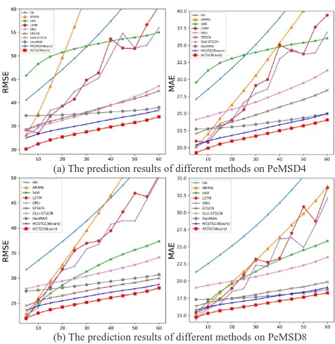
Fig. 6 shows the changes of prediction performance of various methods as the prediction interval increases. Overall, as the prediction interval becomes longer, the correspond-ing difficulty of prediction is gettcorrespond-ing greater, hence the pre-diction errors also increase. As can be seen from the fig-ure, the methods only taking the temporal correlation into account can achieve good results in the short-term predic-tion, such as HA, ARIMA, LSTM and GRU. However, with the increase of the prediction interval, their prediction ac-curacy drops dramatically. By comparison, the performance of VAR drops slower than those methods. This is mainly be-cause VAR can simultaneously consider the spatial-temporal correlations which are more important in the long-term pre-diction. However, when the scale of the traffic network be-comes larger, i.e., there are more time series considered in the model, the prediction error of VAR increases, as shown in Fig.6, its performance on PeMSD4 is worse than that on PeMSD8. The errors of deep learning methods increase slowly with prediction interval increases, and their overall performance is good. Our ASTGCN model achieves the best prediction performance almost all the time. Especially in the long-term prediction, the differences between ASTGCN and other baselines are more significant, showing that the strat-egy of combining attention mechanism with graph

convolu-(b) The prediction results of different methods on PeMSD8 (a) The prediction results of different methods on PeMSD4

Figure 6: Performance changes of different methods as the forecasting interval increases.

tion can better mine the dynamic spatial-temporal patterns of traffic data.

0

1

2

3

4 5

6 7

8

9

Figure 7: The attention matrix obtained from the spatial at-tention mechanism.

Conclusion and Future Work

In this paper, a novel attention based spatial-temporal graph convolution model called ASTGCN is proposed and suc-cessfully applied to forecasting traffic flow. The model combines the spatial-temporal attention mechanism and the spatial-temporal convolution, including graph convolu-tions in the spatial dimension and standard convoluconvolu-tions in the temporal dimension, to simultaneously capture the dy-namic spatial-temporal characteristics of traffic data. Exper-iments on two real-world datasets show that the forecast-ing accuracy of the proposed model is superior to existforecast-ing models. The code has been released at: https://github.com/ wanhuaiyu/ASTGCN.

Actually, the highway traffic flow is affected by many ex-ternal factors, like weather and social events. In the future, we will take some external influencing factors into account to further improve the forecasting accuracy. Since the AST-GCN is a general spatial-temporal forecasting framework for the graph structure data, we can also apply it to other pragmatic applications, such as estimating time of arrival.

Acknowledgments

This work was supported by the Natural Science Foundation of China (No. 61603028).

References

Bruna, J.; Zaremba, W.; Szlam, A.; and Lecun, Y. 2014. Spectral networks and locally connected networks on graphs. In Interna-tional Conference on Learning Representations.

Chen, C.; Petty, K.; Skabardonis, A.; Varaiya, P.; and Jia, Z. 2001. Freeway performance measurement system: mining loop detector data.Transportation Research Record: Journal of the Transporta-tion Research Board(1748):96–102.

Chung, J.; Gulcehre, C.; Cho, K.; and Bengio, Y. 2014. Empiri-cal Evaluation of Gated Recurrent Neural Networks on Sequence Modeling. InNIPS 2014 Workshop on Deep Learning.

Defferrard, M.; Bresson, X.; and Vandergheynst, P. 2016. Con-volutional neural networks on graphs with fast localized spectral filtering. InAdvances in Neural Information Processing Systems, 3844–3852.

Feng, X.; Guo, J.; Qin, B.; Liu, T.; and Liu, Y. 2017. Effective deep memory networks for distant supervised relation extraction. InInternational Joint Conference on Artificial Intelligence, 19–25. He, K.; Zhang, X.; Ren, S.; and Sun, J. 2016. Deep residual learn-ing for image recognition. InIEEE Conference on Computer Vision and Pattern Recognition, 770–778.

Henaff, M.; Bruna, J.; and LeCun, Y. 2015. Deep con-volutional networks on graph-structured data. arXiv preprint arXiv:1506.05163.

Hochreiter, S., and Schmidhuber, J. 1997. Long short-term mem-ory.Neural Computation9(8):1735–1780.

Jeong, Y.-S.; Byon, Y.-J.; Castro-Neto, M. M.; and Easa, S. M. 2013. Supervised weighting-online learning algorithm for short-term traffic flow prediction. IEEE Transactions on Intelligent Transportation Systems14(4):1700–1707.

Kipf, T. N., and Welling, M. 2017. Semi-supervised classification with graph convolutional networks. International Conference on Learning Representations.

Li, C.; Cui, Z.; Zheng, W.; Xu, C.; and Yang, J. 2018. Spatio-Temporal Graph Convolution for Skeleton Based Action Recogni-tion. InAAAI Conference on Artificial Intelligence, 3482–3489. Liang, Y.; Ke, S.; Zhang, J.; Yi, X.; and Zheng, Y. 2018. GeoMAN: Multi-level Attention Networks for Geo-sensory Time Series Pre-diction. InInternational Joint Conference on Artificial Intelligence, 3428–3434.

Niepert, M.; Ahmed, M.; and Kutzkov, K. 2016. Learning convo-lutional neural networks for graphs. InInternational conference on machine learning, 2014–2023.

Shuman, D. I.; Narang, S. K.; Frossard, P.; Ortega, A.; and Van-dergheynst, P. 2013. The emerging field of signal processing on graphs: Extending high-dimensional data analysis to networks and other irregular domains. IEEE Signal Processing Magazine 30(3):83–98.

Simonovsky, M., and Komodakis, N. 2017. Dynamic edgecondi-tioned filters in convolutional neural networks on graphs. In Com-puter Vision and Pattern Recognition, 3693–3702.

Van Lint, J., and Van Hinsbergen, C. 2012. Short-term traffic and travel time prediction models. Artificial Intelligence Applications to Critical Transportation Issues22(1):22–41.

Velickovic, P.; Cucurull, G.; Casanova, A.; Romero, A.; Lio, P.; and Bengio, Y. 2018. Graph attention networks. InInternational Conference on Learning Representations.

Williams, B. M., and Hoel, L. A. 2003. Modeling and forecasting vehicular traffic flow as a seasonal ARIMA process: Theoretical basis and empirical results. Journal of transportation engineering 129(6):664–672.

Xu, K.; Ba, J.; Kiros, R.; Cho, K.; Courville, A.; Salakhudinov, R.; Zemel, R.; and Bengio, Y. 2015. Show, attend and tell: Neural image caption generation with visual attention. InInternational conference on machine learning, 2048–2057.

Yao, H.; Tang, X.; Wei, H.; Zheng, G.; Yu, Y.; and Li, Z. 2018a. Modeling spatial-temporal dynamics for traffic prediction. arXiv preprint arXiv:1803.01254.

Yao, H.; Wu, F.; Ke, J.; Tang, X.; Jia, Y.; Lu, S.; Gong, P.; and Ye, J. 2018b. Deep multi-view spatial-temporal network for taxi demand prediction. InAAAI Conference on Artificial Intelligence, 2588–2595.

Yu, B.; Yin, H.; and Zhu, Z. 2018. Spatio-Temporal Graph Convo-lutional Networks: A Deep Learning Framework for Traffic Fore-casting. In International Joint Conference on Artificial Intelli-gence, 3634–3640.

Zhang, J.; Wang, F.-Y.; Wang, K.; Lin, W.-H.; Xu, X.; and Chen, C. 2011. Data-driven intelligent transportation systems: A sur-vey. IEEE Transactions on Intelligent Transportation Systems 12(4):1624–1639.

Zhang, J.; Zheng, Y.; Qi, D.; Li, R.; Yi, X.; and Li, T. 2018. Pre-dicting citywide crowd flows using deep spatio-temporal residual networks.Artificial Intelligence259:147–166.