R E S E A R C H
Open Access
Modeling the spatial and temporal dynamics of
foraging movements of humpback whales
(
Megaptera novaeangliae
) in the Western
Antarctic Peninsula
Corrie Curtice
1*, David W Johnston
2, Hugh Ducklow
3, Nick Gales
4, Patrick N Halpin
5and Ari S Friedlaender
2,6Abstract
Background:A population of humpback whales (Megaptera novaeangliae) spends the austral summer feeding on Antarctic krill (Euphausia superba)along the Western Antarctic Peninsula (WAP). These whales acquire their annual energetic needs during an episodic feeding season in high latitude waters that must sustain long-distance migration and fasting on low-latitude breeding grounds. Antarctic krill are broadly distributed along the continental shelf and nearshore waters during the spring and early summer, and move closer to land during late summer and fall, where they overwinter under the protective and nutritional cover of sea ice. We apply a novel space-time utilization distribution method to test the hypothesis that humpback whale distribution reflects that of krill: spread broadly during summer with increasing proximity to shore and associated embayments during fall.
Results:Humpback whales instrumented with satellite-linked positional telemetry tags (n = 5), show decreased home range size, amount of area used, and increased proximity to shore over the foraging season.
Conclusions:This study applies a new method to model the movements of humpback whales in the WAP region throughout the feeding season, and presents a baseline for future observations of the seasonal changes in the
movement patterns and foraging behavior of humpback whales (one of several krill-predators affected by climate-driven changes) in the WAP marine ecosystem. As the WAP continues to warm, it is prudent to understand the ecological relationships between sea-ice dependent krill and krill predators, as well as the interactions among recovering populations of krill predators that may be forced into competition for a shared food resource.
Keywords:Humpback whale, Foraging, Western Antarctic Peninsula, Antarctic krill, Satellite telemetry, Space-time utilization distribution, Product kernel
Background
Migratory animals typically spend a portion of their an-nual life cycle in resource-rich feeding grounds [1]. While in these areas, animals typically acquire enough energy to fuel migrations to spatially and temporally dis-parate breeding and calving grounds that are sometimes resource limited. For larger marine mammals such as humpback whales (Megaptera novaeangliae), breeding and feeding grounds are often several thousands of
kilometers apart and require vast amounts of energy and time to transit, highlighting the need to feed efficiently during the time they spend on the foraging grounds.
In marine ecosystems, resources are often patchy in both space and time. In the continental shelf waters along the Western side of the Antarctic Peninsula (WAP), nutri-ent rich circumpolar deep water from the Antarctic Circumpolar current intrudes into coastal areas via a series of deep canyons on the continental shelf [2,3]. This water mixes with phytoplankton-rich and less dense sur-face waters during summer [4], and a resulting lens of nutrient-rich and phytoplankton-laden water is entrained near the surface. Sunlight stimulates algal productivity in * Correspondence:[email protected]
1
Marine Geospatial Ecology Lab, Nicholas School of the Environment, Duke University Marine Laboratory, Beaufort, NC 28516, USA
Full list of author information is available at the end of the article
these waters, which is subsequently consumed by a myriad of lower and, eventually, upper trophic level predators [4].
Humpback whales are the most numerous baleen whale found in the nearshore waters along the WAP [5-8]. These whales breed in tropical waters near the equator in winter and feed during summer months in the high-latitude Antarctic waters [9]. Because of their large body size (adults reach up to 15 meters long and 40 tons in weight), they have extremely high energetic demands. These needs are met through an anatomically evolved bulk-filter feeding mechanism that allows them to process a volume of prey-laden water nearly equal to their body mass in a single feeding lunge [10]. Antarctic krill (Euphausia superba) are the dominant macro-zooplankton in WAP waters and are the primary com-ponent of humpback whale diets in this area [11]. Previous work has shown that the distribution and abun-dance of humpback whales around the WAP are best predicted by that of Antarctic krill [12]. As mobile pred-ators with high energetic demands, it stands to reason that humpback whales will seek out areas with increased prey abundance, changing their distribution to reflect such prey changes throughout the feeding season.
During summer months Antarctic krill are abundant both at the marginal ice edge zone as winter sea ice re-treats and throughout open continental shelf waters [13]. A portion of the adult population of krill can also be found offshore, where they deposit their eggs in deep water [13]. Thus, during summer months, krill are dis-tributed broadly from nearshore to beyond the continen-tal shelf. In autumn, krill appear to move inshore and towards sheltered bays where they coalesce into large ag-gregations that will be covered by sea ice formation [13], minimizing predation risk from diving predators includ-ing baleen whales [7,14]. It is also believed that the under-ice habitat offers ample food to feed juvenile krill over the winter [13]. Sea ice formation varies both latitu-dinally along the WAP and annually, especially along the western side of the Antarctic Peninsula, generally reach-ing its greatest extent between July-September [15].
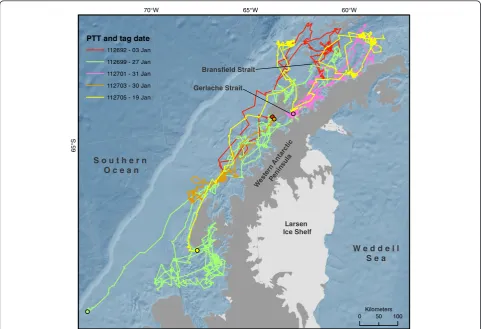
Previous research on humpback whales in the Gerlache and Bransfield Strait areas of the WAP (see Figure 1 for these locations) found that whales exhibited both short and long-distance movements with relatively short resi-dency times and variable-sized home ranges between pre-sumed foraging areas during summer [16]. Recently,
60°W 65°W
70°W
65°
S
0 50 100
Kilometers
West ern
Ant arct
ic
Pen insu
la
Larsen Ice Shelf S o u t h e r n
O c e a n
W e d d e l l S e a PTT and tag date
112692 - 03 Jan
112699 - 27 Jan
112701 - 31 Jan
112703 - 30 Jan 112705 - 19 Jan
Gerlache Strait Bransfield Strait
exceptional aggregations of both Antarctic krill [17] and humpback whales have been observed in nearshore bays late in the feeding season [7], with higher densities of whales than previously reported in these locations [8]. Given the known distribution of whales in summer months and the ultimate disposition of both whales and krill later in the feeding season, we hypothesize that the movement patterns and home ranges of humpback whales will reflect seasonal changes in the distribution and behav-ior of Antarctic krill. Specifically we predict that the area of whale movements will decrease over time, and that the overall distribution of humpback whales will become more proximate to shore over our study period, from the beginning of summer (January) to the end of the feeding season (June).
To test these predictions, we examined the spatial dis-persion and coastal proximity of time-variant home ranges derived from satellite locations of Antarctic humpback whales in the WAP. Probabilistic home ranges are commonly used to describe an animal’s use of space [18], giving a probability of occurrence for an area. Van Winkle [19] described these as utilization distribu-tions (UD) derived from two-dimensional animal loca-tions, and Worton [20] describes the kernel estimator [21] as a robust, non-parametric, probability density function for determining the UD. Keating and Cherry [22] have expanded Van Winkle’s UD definition to in-clude four dimensions, adding time and elevation (or depth in the case of marine animals), and expanded the traditional kernel method into a new“product kernel al-gorithm”. Here we applied this new product kernel method to a new taxonomic group (baleen whales) in a novel region (Antarctic Peninsula) and derived measures of space use to better understand the temporal move-ment patterns and behavior of these mobile ocean pred-ators in a dynamic environment.
Results
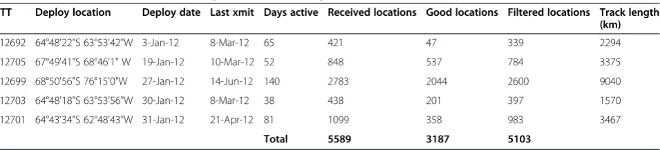
Five satellite-linked tags (Platform Transmitting Termi-nals [PTTs]) were deployed and remained active for be-tween 38 and 140 days (Table 1; Figure 1). All of the
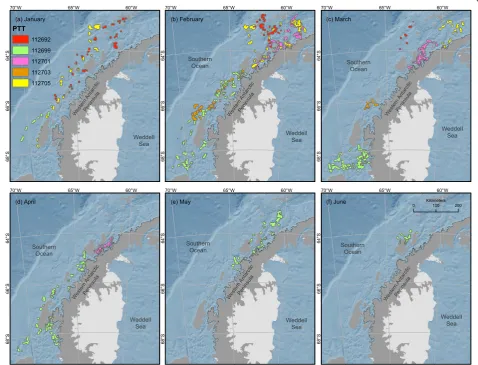
PTTs were deployed during January 2012, with a differ-ence of 28 days between the first and last deployments. Three PTTs (112692, 112703, 112705) stopped transmit-ting in early March (8 March, 8 March and 10 March re-spectively), and have the shortest durations (65, 38, and 52 days respectively) and are therefore skewed towards the beginning of the summer. The two remaining PTTs (112699, 112701) were the longest duration (140 and 81 days respectively), covering a later and longer period of the feeding season. Track lengths ranged from 1570 km to 9040 km (Table 1), providing a general measure of how much each whale moved. The quality of locations (Argos’ “Location Class”) equal to or greater than class 0 (the set of classes which have estimated error ranges associated with them) comprised 60% of the total locations used in the analysis (Table 1). Home ranges, defined as the 95% Utilization Distribution (UD) calculated with a spatio-temporal kernel density algo-rithm, were calculated for each of the five whales at up to 75 specific time steps, depending on the duration of the PTT (Figure 2).
Model results
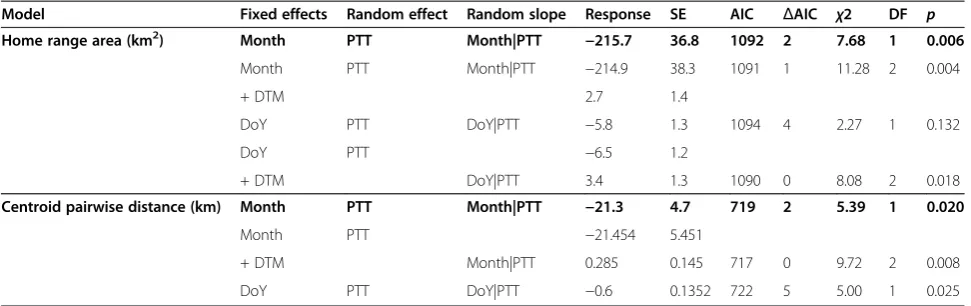
All tested models used Day of Year or month with and without distance to mainland as potential fixed effects predictors, and all tested models used PTT as a random effect to account for individual whale variations in movement (see Table 2 for full model results). Each model also included the temporal fixed effect (Day of Year or month) as a random slope. When AIC values for models were within two AIC units of the model with the lowest AIC score, the most simplistic model of that set was chosen [23]. Models were also evaluated based on the p-value and chi-square results when compared via the ANOVA (analysis of variance) likelihood ratio test to a “null” model with only distance to mainland as the fixed effect.
Three of the four home range area models showed sig-nificant difference from the null models and were within two AIC units of the model with the lowest AIC; the se-lected model with only month as a predictor (χ2(1) =
Table 1 Details of Platform Transmitting Terminal (PTT) tags
PTT Deploy location Deploy date Last xmit Days active Received locations Good locations Filtered locations Track length (km)
112692 64°48'22"S 63°53'42"W 3-Jan-12 8-Mar-12 65 421 47 339 2294
112705 67°49'41"S 68°46'1" W 19-Jan-12 10-Mar-12 52 848 537 784 3375
112699 68°50'56"S 76°15'0"W 27-Jan-12 14-Jun-12 140 2783 2044 2600 9040
112703 64°48'18"S 63°53'56"W 30-Jan-12 8-Mar-12 38 438 201 397 1570
112701 64°43'34"S 62°48'43"W 31-Jan-12 21-Apr-12 81 1099 358 983 3467
Total 5589 3187 5103
7.68, p= 0.006) was the most parsimonious of the three. With each increase in month, there was a corresponding decrease in home range area of 215.7 km2± 36.8 km2 (standard errors). The models with distance to mainland as predictors also show that as distance to mainland in-creased, the home range area also inin-creased, indicating that when further from the mainland the whales range over a larger area.
The distances between the centroids of each home range area for each whale is a measure for the range or spread of each whale over the course of the foraging sea-son [24]. If the whales move closer to shore, presumably following the movement of krill, the distances between the 95% UD polygons (representing the general “home range” for the 5-day spread around a given date) should decrease over time. Three models showed significant
differences from the null models (one model failed to converge); the selected model with only month as the predictor (χ2(1) = 5.39, p= 0.02) was more parsimonious than the lowest AIC scoring model. For each increase in month the model shows a corresponding decrease in the pairwise distance of centroids of 21.3 km ± 4.7 km (standard errors).
Discussion
The results of our spatial analyses indicate that the dis-tribution and movement patterns of satellite-tagged humpback whales on Antarctic foraging grounds change significantly over the course of the feeding sea-son (approximately January to June). Both of our spatial metrics - time-variant home range area and pairwise home range centroid distance - decrease as a function 60°W 65°W 70°W 64° S 66° S 68° S 60°W 65°W 70°W 64° S 66° S 68° S 60°W 65°W 70°W 6 4 °S 6 6° S 6 8 °S We ster nA nta rctic Peni nsul a Southern Ocean Weddell Sea
(a) January (c) March
West ern Anta rctic Penin sula Southern Ocean Weddell Sea (b) February West ern Ant arct ic Peni nsul a 60°W 65°W 70°W 64° S 6 6 °S 68° S 60°W 65°W 70°W 64° S 66° S 68° S 60°W 65°W 70°W 6 4 °S 6 6° S 68° S
(d) April (e) May (f) June
Southern Ocean
Southern
Ocean SouthernOcean
Weddell Sea
Weddell
Sea WeddellSea
Weddell Sea 0 Kilometers100 200 PTT 112692 112699 112701 112703 112705 Wes tern Ant arc tic Penin sula We ster nAn tarc tic Peni nsu la We ste rnAnt arcti c Peni nsul a
of time and proximity to shore. We believe that these results are additional evidence that humpback whales move in concert with seasonal changes in the broad-scale distribution of their main prey, Antarctic krill [13]. During January, the time of our PTT deployments, krill are generally dispersed across the nearshore and continental shelf waters of the WAP [14]. Over the course of the summer months, krill have been shown to move inshore and aggregate into denser patches [7,14]. Based on these previous studies of krill movement, our results provide supporting evidence that whales track the movement of their primary prey through the summer months, adjusting their movements to maintain proximity to this important resource, resulting in increased whale density in the nearshore regions of the WAP [8].
In the WAP region, a suite of predators relies on krill as a primary food item. In addition to baleen whales (including humpback, minke whales - Balaenoptera bonaerensis, and fin whales - Balaenoptera physalus), several penguin, seabird and seal species acquire the vast majority of their energy from Antarctic krill [25]. While these animals share a common prey, they exhibit markedly differently life history strategies that affect their foraging patterns and movement ecology. For ex-ample, during summer months, Adelie penguins ( Pygos-celis adeliae) and gentoo penguins (Pygoscelis papua) are considered central-place foragers that come and go from terrestrial nesting sites frequently to provision and rear growing chicks. This requires the penguins to stay in close spatial proximity (15–60 km [26,27]) to such areas, and the breeding success of penguins at a par-ticular breeding rookery depends largely on local krill abundance [28]. Crabaeater (Lobodon carcinophagus), leopard (Hydrurga leptonyx), and Antarctic fur seals
(Arctocephalus gazella) also rely on krill as a food item in this region [29]. While they are not necessarily dependent on returning to rookeries to provision pups, they are limited in their foraging ranges by the presence of suitable haul-out areas where they can rest and avoid predators. These typically take the form of sea ice floes or rocky coastlines. Therefore, like penguins, krill-dependent seals are limited in their foraging ranges by physical substrate rather than directly by the distribu-tion of their prey [12].
In contrast, humpback whale distribution is best pre-dicted by the distribution of their prey [6], and these whales are not bound by the constraints of central place foragers [12]. Humpback whales spend summer months on foraging grounds replenishing lost energy and adding additional energy stores to fuel long distance migrations to tropical calving/breeding grounds [9]. Because they typically do not feed during migrations or on their breeding/calving grounds, humpback whales must ac-quire enough energy during summer months to support their energetic demands for the entire year [30]. It is therefore important for them to maximize their time on feeding grounds and maintain proximity to the highest densities of prey available to them. Our results support previous work that was based on visual sightings of whales over short periods of time [7,8,12,31], and poten-tially increases our understanding of the spatial relation-ship between humpback whales and krill over longer time periods. Linking work of long duration satellite tags with long duration observations of krill distribution [31], sea ice [15] and oceanographic conditions [32] will deepen this understanding.
While krill can be found in the nearshore waters around the WAP during summer months, they are also
Table 2 Model results for home range area and centroid pairwise distance
Model Fixed effects Random effect Random slope Response SE AIC ΔAIC χ2 DF p
Home range area (km2) Month PTT Month|PTT −215.7 36.8 1092 2 7.68 1 0.006
Month PTT Month|PTT −214.9 38.3 1091 1 11.28 2 0.004
+ DTM 2.7 1.4
DoY PTT DoY|PTT −5.8 1.3 1094 4 2.27 1 0.132
DoY PTT −6.5 1.2
+ DTM DoY|PTT 3.4 1.3 1090 0 8.08 2 0.018
Centroid pairwise distance (km) Month PTT Month|PTT −21.3 4.7 719 2 5.39 1 0.020
Month PTT −21.454 5.451
+ DTM Month|PTT 0.285 0.145 717 0 9.72 2 0.008
DoY PTT DoY|PTT −0.6 0.1352 722 5 5.00 1 0.025
P-value andχ2 values were obtained by analysis of variance tests of each of the full models against a null model. Null models had Distance To Mainland (DTM) as the only fixed effect, to determine if month or Day of Year (DoY) was a significant predictor variable. DoY + DTM centroid pairwise distance model failed to converge and has been omitted. The Platform Transmitting Terminal (PTT) is unique to each whale, and was used as a random effect with by-whale random slope to capture the variation in movements between individual whales. Response is the unit change in the dependent variable (home range area in km2
or centroid pairwise distance in km) per unit increase in the fixed effect variable(s). For example, for each unit increase in month, the home range area decreased by 215.7 km2
with a standard error of ±36.8 km2
more specifically distributed in relation to several phys-ical features that likely enhance local productivity. Krill are known to feed and aggregate at the marginal sea ice edge as ice retreats [13], and it has also been hypothe-sized that krill aggregate proximate to deep water can-yons that allow nutrient-rich Circumpolar Deep water to move inshore and be upwelled, creating ideal conditions for primary producers and consumers [3]. This notion that, over time, these deep canyons provide predictable food resources for krill predators has been the focus of several long-term studies on the location of penguin rookeries around the WAP [28,33]. As the long photo-period of summer months begins to wane, it is believed that Antarctic krill begin to move inshore and into areas where they will overwinter [14]. Several studies have documented this offshore-inshore migration of krill into nearshore bays where krill eventually coalesce into massive aggregations [7,14]. It is theorized that krill make these inshore migrations to seek shelter under the cover of annual sea ice that limits access from air-breathing predators, and allows them to survive in large, dense aggregations until the following spring. Gerlache strait, a focal area in our study, is consistently the last part of the WAP to be covered with sea ice, typically be-ginning around June, giving whales longer foraging ac-cess to the aggregated krill [13].
Humpback whales are known to feed (via lunging) be-tween 300–900 times in a 24-hour period, and must re-cover the energy used by feeding on high densities of krill [34]. It is likely then that humpback whales will graze local krill abundances below a level that is no lon-ger energetically profitable and will move to a new loca-tion to feed when this level is reached [35]. During summer months it appears that krill are patchy and dis-tributed in discrete aggregations across the southern WAP region and along the shelf break [36,37] and humpback whales would likely need to move frequently in search of suitable prey densities. The results of our analyses support this hypothesis, with whales having lar-ger foraging ranges that are farther from the coastline earlier in the feeding season. The movement patterns of the tagged humpback whales in this study therefore may reflect the general pattern of seasonal krill movements, from a lower density offshore distribution into higher density near shore aggregations [7].
Our methods provide a metric to assess time-space use of a large and mobile marine predator. The new methods used in this study which show the progression of animal space use over time, could, in concert with concurrent prey studies lead to a new approach to evalu-ating the ecological relationship between predators and their prey (or other environmental features that provide context for behaviors) and may be applicable to a broad range of taxonomic groups in marine ecosystems.
Caveats and considerations
Previously determined ecological relationships between humpback whales and krill in the WAP region provide for strong inference that the primary driver affecting the distribution and movement pattern of these whales is in-deed that of Antarctic krill [6,12]. A competing hypoth-esis regarding the observed movement patterns of humpback whales is that the animals will, over time, graze down krill resources below a profitable threshold level (marginal value theory) and move from patch to patch in order to satisfy their energetic demands [35,38]. Currently, baleen whales are still at a fraction of their historic population levels and there is no evidence to suggest that krill are a limited resource in the area [39]. Thus, while whales are likely to graze patches at a very local level, their ability to diminish resources across a broad area is unlikely. If this were the case, whales would increase their search radius over time to find resources outside of where they have already grazed, something that is not supported by the data we have presented.
Our results only provide information for a single year, with a modest sample size, and there is likely to be inter-annual variability in environmental conditions in this region that may influence the magnitude of the rela-tionship between krill distributions and the space use of humpback whales. However, there are no data to suggest that the previously determined relationships between the distribution of whales and krill will fundamentally change over such short time frames.
PTT deployments were generally of short duration, with only two of the five reporting data after early March. Since we are trying to capture changes in behav-ior throughout the course of the feeding season, which can last into June in this area of the WAP, it is possible that the three shorter deployments are not fully captur-ing the transition towards more constricted, near shore movements. Longer deployments would help address this consideration, and help support our theory that the constricting use of space over time applies broadly to the humpback whales foraging along the WAP.
Other environmental parameters also contribute to humpback whale distribution (e.g. sea surface temperature, deep temperature maximum, amount and extent of sea ice cover) however several analytic models all show krill as the most significant determinate [6,12]. Examination of the Passive Microwave Data from the National Snow & Ice Data Center for the months of this study (January–June 2012) show the Gerlache and Bransfield Straits areas to be ice free from February through sometime in June [40], supporting our theory that the whales are follow-ing their prey, and not alterfollow-ing their home ranges over time to avoid ice cover.
battery degradation and related transmission loss altered the outcome of our analysis. In this study, the tags were programmed to conserve the life of two lithium ion bat-teries on-board the tag by duty cycling on for four hours, then off for eight hours. A reduction in battery power over time may potentially alter the number of successful transmissions, however our data show only a slight degradation of transmission rate. It’s more likely that the tags stopped transmitting after catastrophic fail-ures such as the tag falling off, salt water invasion in the tag, or antennae fouling or breaking. Other factors could also confound transmission rate, such as the behavior of the whale –if actively feeding the whale will spend less time at the surface, giving less opportunity for a location to be obtained [34].
Conclusions
Despite the small sample size, this study provides initial results of how the movements of humpback whales in the WAP region are likely related to the seasonal change in distribution of their primary prey, Antarctic krill. Our application of a novel method for showing changes in space use over time present a baseline for future obser-vations of the seasonal changes in the movement pat-terns and foraging behavior of humpback whales, and potentially other Antarctic krill predators. The amount and persistence of sea ice around the western side of the WAP has decreased significantly since 1979 [41] while air temperatures have risen [42]. The life history of Antarctic krill is intimately tied to sea ice cover and the documented changes that we are currently witnes-sing have been implicated in the decrease of krill in this region [43]. As conditions continue to change, it is pru-dent to understand the ecological relationships between krill and krill predators in the WAP as well as interac-tions among krill predators that may be increasingly subjected to competition for a shared food resource.
Methods
During January 2012, Wildlife Computer (Redmond, WA, USA) SPOT5 Platform Transmitting Terminals (PTTs) were attached to six humpback whales in the continental shelf waters of the WAP (Figure 1) [44]. Each PTT is contained in a stainless steel custom hous-ing that penetrates the whale’s skin and hypodermis up to 290 mm deep, and is anchored in the tissues beneath the blubber layer with stainless steel foldable barbs. PTTs were kept in sealed sterilized packages until de-ployment from a Mark V Zodiac rigid-hulled inflatable boat with a 40-hp 4-stroke engine using a compressed air gun set at a pressure between 7.5 and 10 bar. Whales were approached at idle speed and from a perpendicular or oblique rear angle to reduce disturbance, and the PTTs were deployed at a range of 3-8 m. PTTs were
placed high on the dorsal surface of the whale, in the vicinity of the dorsal fin, to maximize antenna exposure each time the animal surfaced. The dorsal fins and flukes of each tagged animal were photographed for individual identification.
SPOT5 PTTs are satellite linked via the Argos System. All were programmed to transmit daily during the hours 00:00 to 04:00 and 12:00 to 16:00 (GMT) and were acti-vated via the salt-water switch with the first dive after tagging. Locations obtained through Argos have varying levels of estimated error. Each location is coded with a location class (LC) starting with Z, B, and A which have no predicted estimated error, and LC 0, 1, 2, and 3 which have an associated 1-sigma error radius of ap-proximately >1500 m, <1500 m, <500 m, and <250 m, respectively [45]. Locations with an LC of Z were not cluded in the analysis because they are considered in-valid by Argos. Remaining locations were filtered using the sdafilter function in the argosfilter [46] package in the R development environment [47] to remove improb-able locations based on swimming speed, distance be-tween locations, and turning angle bebe-tween locations. A maximum estimated swimming speed of 5 m/s was used. All locations were projected to UTM Zone 20 South. Location points for each PTT were transformed into track lines using the “Points to Line” tool [48], and the length calculated via the calculate geometry tool. One track that was only three days in duration was removed from the data set.
To evaluate changes in habitat use of tagged hump-back whales over the feeding season, we used a robust product kernel method [22] as implemented in the ade-habitat package for R [49]. This method extends the traditional utilization distribution (UD) method [21] by allowing four dimensions to be modeled (x, y, z, t), wherezrepresents elevation/depth andtrepresents time in either linear or circular units. The tags used in this study did not record dive behavior, so the z dimension was not used in this analysis. Bandwidths were chosen for x and y as 5000 m, and for tas 5-days, each based on initial exploration of the data [21].
(excluding islands), hereafter referred to as DTM. These values were then averaged for each whale for each time-smoothed UD around each date to get a sin-gle per-date DTM, to be used in the regression model-ing. The area of the combined 95% UD polygons (the total summed home range) for each whale on each date was used for regression modeling. Additionally, we av-eraged the pairwise distances (PWD) of the centroids among multiple polygons for each date for each whale to get a quantitative measure of each respective UD’s spatial spread. These values represent the total range of a whale in a given 10-day period (the date of the UD smoothed by 5 days); our hypothesis indicates that these values should also decrease over the duration of the summer feeding season, as the whales spend in-creasing amounts of time in smaller areas feeding on krill aggregations.
We used R and lme4 [51] to perform linear mixed ef-fects analyses to model humpback whale home range area and PWD. DTM, Day of Year and month were used as potential fixed effects, and the PTT was used as a random effect with by-whale random slopes. P-values were obtained by ANOVA (analysis of variance) likeli-hood ratio tests of each of the full models against a null model with DTM as the only fixed effect.
Competing interests
The authors have declared there are no competing interests.
Authors’contributions
CC performed statistical analyses of data, created all figures, drafted manuscript, presented findings at symposium. DWJ conceived the work, provided guidance and input on data analyses, drafted manuscript. ASF conceived the work, deployed tags, provided input to data analyses, and drafted the manuscript. PH, NG and HD contributed to logistical and field support and edited the manuscript. All authors read and approved the final manuscript.
Acknowledgements
All whale research was conducted under grant award ANT-0823101 and NMFS permit 14097, ACA permit 2009–013, and Duke University IACUC A049-112-02. Research was conducted under a collaboration with the National Science Foundation Office of Polar Program’s Palmer Long-term Ecological Research Program and the Australian Antarctic division, and we thank the investigators of this project for their support. We would also like to thank the Captain, crew, and marine technicians of theARSV Laurence M Gould
for their support. Three anonymous reviewers contributed greatly to the strength and clarity of this manuscript.
Author details
1
Marine Geospatial Ecology Lab, Nicholas School of the Environment, Duke University Marine Laboratory, Beaufort, NC 28516, USA.2Division of Marine
Science and Conservation, Nicholas School of the Environment, Duke University Marine Laboratory, Beaufort, NC 28516, USA.3Lamont Doherty
Earth Observatory, Columbia University, Palisades, NY 10964, USA.4Australian Antarctic Division, Kingston, TAS, Australia.5Marine Geospatial Ecology Lab,
Nicholas School of the Environment, Duke University, Durham, NC 27708, USA.6Marine Mammal Institute, Hatfield Marine Science Center, Oregon
State University, Newport, OR 97365, USA.
Received: 4 November 2014 Accepted: 27 April 2015
References
1. Dingle H: Migration: the Biology of Life on the Move. New York City, NY: Oxford University Press; 1996.
2. Dinniman MS, Klinck JM, Smith Jr WO. A model study of Circumpolar Deep Water on the West Antarctic Peninsula and Ross Sea continental shelves. Deep-Sea Res Pt Ii. 2011;58:1508–23.
3. Klinck JM, Hofmann EE, Beardsley RC, Salihoglu B, Howard S. Water-mass properties and circulation on the west Antarctic Peninsula Continental Shelf in Austral Fall and Winter 2001. Deep-Sea Res Pt Ii. 2004;51:1925–46. 4. Prézelin BB, Hofmann EE, Mengelt C, Klinck JM. The linkage between Upper
Circumpolar Deep Water (UCDW) and phytoplankton assemblages on the west Antarctic Peninsula continental shelf. Journal Of Marine Research. 2000;58:165–202.
5. Thiele D, Chester E, Moore SE, Sirovic A, Hildebrand JA, Friedlaender A. Seasonal variability in whale encounters in the Western Antarctic Peninsula. Deep-Sea Res Pt Ii. 2004;51:2311–25.
6. Friedlaender A, Halpin P, Qian S, Lawson G, Wiebe P, Thiele D, et al. Whale distribution in relation to prey abundance and oceanographic processes in shelf waters of the Western Antarctic Peninsula. Mar Ecol Prog Ser. 2006;317:297–310. 7. Nowacek DP, Friedlaender AS, Halpin PN, Hazen EL, Johnston DW, Read AJ, et al. Super-Aggregations of Krill and Humpback Whales in Wilhelmina Bay, Antarctic Peninsula. PLoS ONE. 2011;6, e19173.
8. Johnston DW, Friedlaender AS, Read AJ, Nowacek DP. Initial density estimates of humpback whales Megaptera novaeangliae in the inshore waters of the western Antarctic Peninsula during the late autumn. Endang Species Res. 2012;18:63–71.
9. Robbins J, Dalla Rosa L, Allen JM, Mattila DK, Secchi ER, Friedlaender AS, et al. Return movement of a humpback whale between the Antarctic Peninsula and American Samoa: a seasonal migration record. Endang Species Res. 2011;13:117–21.
10. Potvin J, Goldbogen JA, Shadwick RE. Scaling of lunge feeding in rorqual whales: an integrated model of engulfment duration. J Theor Biol. 2010;267:437–53.
11. Mackintosh NA. The Stocks of Whales. London, UK: Fishing News Books; 1965. 12. Friedlaender AS, Johnston DW, Fraser WR, Burns J, Patrick NH, Costa DP.
Ecological niche modeling of sympatric krill predators around Marguerite Bay, Western Antarctic Peninsula. Deep-Sea Res Pt Ii. 2011;58:1729–40. 13. Nicol S. Krill, Currents, and Sea Ice: Euphausia superba and Its Changing
Environment. Bioscience. 2006;56:111–20.
14. Lascara CM, Hofmann EE, Ross RM, Quetin LB. Seasonal variability in the distribution of Antarctic krill, Euphausia superba, west of the Antarctic Peninsula. Deep-Sea Res Pt I. 1999;46:951–84.
15. Stammerjohn S, Massom RA, Rind D, Martinson DG. Regions of rapid sea ice change: An inter-hemispheric seasonal comparison. Geophys Res Lett. 2012;39, L06501.
16. Dalla Rosa L, Secchi ER, Maia YG, Zerbini AN, Heide-Jorgensen MP. Move-ments of satellite-monitored humpback whales on their feeding ground along the Antarctic Peninsula. Polar Biol. 2008;31:771–81.
17. Espinasse B, Zhou M, Zhu Y, Hazen EL, Friedlaender AS, Nowacek DP, et al. Austral fall−winter transition of mesozooplankton assemblages and krill aggregations in an embayment west of the Antarctic Peninsula. Mar Ecol Prog Ser. 2012;452:63–80.
18. Worton BJ. A review of models of home range for animal movement. Ecol Model. 1987;38:277–98.
19. Van Winkle W. Comparison of several probabilistic home-range models. The Journal of wildlife management 1975;39(1):118–123.
20. Worton BJ. Kernel methods for estimating utilization distribution in home-range studies. Ecology. 1989;70:164–8.
21. Silverman BW. Density Estimation for Statistics and Data Analysis. London, UK: Chapman & Hall; 1986.
22. Keating KA, Cherry S. Modeling utilization distributions in space and time. Ecology. 2009;90:1971–80.
23. Arnold TW. Uninformative Parameters and Model Selection Using Akaike’s Information Criterion. J Wildlife Manage. 2010;74:1175–8.
24. Boustany AM, Matteson R, Castleton M, Farwell C, Block BA. Progress in Oceanography. Prog Oceanogr. 2010;86:94–104.
25. Knox GA. Biology of the Southern Ocean. 2nd ed. Boca Raton, FL: CRC Press/Taylor & Francis; 2006.
27. Wilson RP, Nagy KA, Obst BS. Foraging ranges of penguins. Polar Record. 1989;25:303–8.
28. Fraser WR, Hofmann EE. A predator’s perspective on causal links between climate change, physical forcing and ecosystem response. Mar Ecol Prog Ser. 2003;265:1–15.
29. Costa DP, Crocker D. Marine mammals of the Southern Ocean. In: Ross R, Hofmann EE, Quetin LB, editors. Foundations for Ecological Research West of the Antarctic Peninsula. 1996. p. 287–301.
30. Clapham PJ, Young SB, Brownell RL. Baleen whales: conservation issues and the status of the most endangered populations. Mammal Rev. 1999;29:37–62. 31. Ross RM, Quetin LB, Martinson DG, Iannuzzi RA, Stammerjohn SE, Smith RC.
Palmer LTER: Patterns of distribution of five dominant zooplankton species in the epipelagic zone west of the Antarctic Peninsula. Deep-Sea Res Pt Ii. 2008;55:2086–105.
32. Ducklow HW, Fraser W, Karl DM, Quetin LB, Ross RM, Smith RC, et al. Water-column processes in the West Antarctic Peninsula and the Ross Sea: Interannual variations and foodweb structure. Deep-Sea Res Pt Ii. 2006;53:834–52.
33. Oliver MJ, Irwin A, Moline MA, Fraser W, Patterson D, Schofield O, et al. Adélie Penguin Foraging Location Predicted by Tidal Regime Switching. PLoS One. 2013;8, e55163.
34. Friedlaender AS, Tyson RB, Stimpert AK, Read AJ, Nowacek DP. Extreme diel variation in the feeding behavior of humpback whales along the western Antarctic Peninsula during autumn. Mar Ecol Prog Ser. 2013;494:281–9. 35. Piatt JF, Methven DA. Threshold foraging behavior of baleen whales. Mar
Ecol Prog Ser. 1992;84:205–10.
36. Lawson GL, Wiebe PH, Stanton TK, Ashjian CJ. Euphausiid distribution along the Western Antarctic Peninsula—Part A: Development of robust multi-frequency acoustic techniques to identify euphausiid aggregations and quantify euphausiid size, abundance, and biomass. Deep-Sea Res Pt Ii. 2008;55:412–31.
37. Ashjian CJ, Davis CS, Gallager SM, Wiebe PH, Lawson GL. Distribution of larval krill and zooplankton in association with hydrography in Marguerite Bay, Antarctic Peninsula, in austral fall and winter 2001 described using the Video Plankton Recorder. Deep-Sea Res Pt Ii. 2008;55:455–71.
38. Charnov EL. Optimal foraging, the marginal value theorem. Theor Popul Biol. 1976;9:129–36.
39. Clapham PJ, Brownell RL. The potential for interspecific competition in baleen whales. Reports of the International Whaling Commission. 1996;46:361–7.
40. Sea ice concentrations from Nimbus-7 SMMR and DMSP SSMI passive microwave data. Accessed on January 30 2015 [http://nsidc.org/] 41. Stammerjohn SE, Martinson DG, Smith RC, Iannuzzi RA. Sea ice in the
western Antarctic Peninsula region: Spatio-temporal variability from ecological and climate change perspectives. Deep-Sea Res Pt Ii. 2008;55:2041–58. 42. Vaughan DG, Marshall GJ, Connolley WM, Parkinson C, Mulvaney R,
Hodgson DA, et al. Recent Rapid Regional Climate Warming on the Antarctic Peninsula. Clim Change. 2003;60:243–74.
43. Atkinson A, Siegel V, Pakhomov E, Rothery P. Long-term decline in krill stock and increase in salps within the Southern Ocean. Nature. 2004;432:100–3. 44. Friedlaender AS, Curtice C, Ducklow HW, Halpin PN, Johnston DW, Gales NJ.
Long Term Ecological Research: Satellite Telemetry of Humpback Whale Movements in the Antarctic Peninsula. OBIS-SEAMAP. 2015. http://seama-p.env.duke.edu/dataset/1261.
45. Argos User’s Manual v1.6.4. www.argos-system.org/manual. Accessed 23 Mar 2015.
46. Freitas C, Lydersen C, Fedak MA, Kovacs KM. A simple new algorithm to filter marine mammal Argos locations. Mar Mam Sci. 2008;24:315–25. 47. R Core Team. R: A language and environment for statistical computing. Vienna,
Austria: R Foundation for Statistical Computing. 2015. http://www. r-project.org.
48. Environmental Systems Research Institute. ArcGIS Desktop: Release 10.2. Redlands, CA. 2014.
49. Calenge C. The package adehabitat for the R software: a tool for the analysis of space and habitat use by animals. Ecological Modelling. 2006;197:516–19.
50. Antarctic Digital Database Version 6.0 http://www.add.scar.org. Accessed 23 Mar 2015.
51. Bates D, Maechler M, Bolker B, Walker S. lme4: Linear mixed-effects models using Eigen and S4. R package version 1.1-7. 2014. cran.r-project.org/ package=lme4.
Submit your next manuscript to BioMed Central and take full advantage of:
• Convenient online submission
• Thorough peer review
• No space constraints or color figure charges
• Immediate publication on acceptance
• Inclusion in PubMed, CAS, Scopus and Google Scholar
• Research which is freely available for redistribution