Open Access
Research article
Combining estimates of interest in prognostic modelling studies
after multiple imputation: current practice and guidelines
Andrea Marshall*
1,2, Douglas G Altman
1, Roger L Holder
3and
Patrick Royston
4Address: 1Centre for Statistics in Medicine, University of Oxford, Oxford, UK, 2Warwick Clinical Trials Unit, University of Warwick, Coventry, UK, 3Department of Primary Care & General Practice, University of Birmingham, Birmingham, UK and 4Hub for Trials Methodology Research and UCL, MRC Clinical Trials Unit, London, UK
Email: Andrea Marshall* - [email protected]; Douglas G Altman - [email protected]; Roger L Holder - [email protected]; Patrick Royston - [email protected]
* Corresponding author
Abstract
Background: Multiple imputation (MI) provides an effective approach to handle missing covariate data within prognostic modelling studies, as it can properly account for the missing data uncertainty. The multiply imputed datasets are each analysed using standard prognostic modelling techniques to obtain the estimates of interest. The estimates from each imputed dataset are then combined into one overall estimate and variance, incorporating both the within and between imputation variability. Rubin's rules for combining these multiply imputed estimates are based on asymptotic theory. The resulting combined estimates may be more accurate if the posterior distribution of the population parameter of interest is better approximated by the normal distribution. However, the normality assumption may not be appropriate for all the parameters of interest when analysing prognostic modelling studies, such as predicted survival probabilities and model performance measures.
Methods: Guidelines for combining the estimates of interest when analysing prognostic modelling studies are provided. A literature review is performed to identify current practice for combining such estimates in prognostic modelling studies.
Results: Methods for combining all reported estimates after MI were not well reported in the current literature. Rubin's rules without applying any transformations were the standard approach used, when any method was stated.
Conclusion: The proposed simple guidelines for combining estimates after MI may lead to a wider and more appropriate use of MI in future prognostic modelling studies.
Background
Prognostic models play an important role in the clinical decision making process as they help clinicians to deter-mine the most appropriate management of patients. A good prognostic model can provide an insight into the
relationship between the outcome of patients and known patient and disease characteristics [1,2].
Missing covariate data and censored outcomes are unfor-tunately common occurrences in prognostic modelling Published: 28 July 2009
BMC Medical Research Methodology 2009, 9:57 doi:10.1186/1471-2288-9-57
Received: 11 March 2009 Accepted: 28 July 2009
This article is available from: http://www.biomedcentral.com/1471-2288/9/57
© 2009 Marshall et al; licensee BioMed Central Ltd.
studies [3], which can complicate the modelling process. Multiple imputation (MI) is one approach to handle the missing covariate data that can properly account for the missing data uncertainty [4]. Missing values are replaced with m (>1) values to give m imputed datasets. Previously, three to five imputations were considered sufficient to give reasonable efficiency provided that the fraction of missing information is not excessive [4]. However, with increased computer capabilities, the limitations on m have diminished and therefore it may be more sensible to use 20 [5] or more [6] imputations. The imputation model, used to generate plausible values for the missing data, should contain all variables to be subsequently ana-lysed including the outcome and any variables that help to explain the missing data [7]. Outcome tends to be incorporated into the imputation model by including both the event status, indicating whether the event, i.e. death, has occurred or not, and the survival time, with the most appropriate transformation [7]. Due to censoring, this approach is not exact and may introduce some bias, but should still help to preserve important relationships in the data. The m imputed datasets are each analysed using standard statistical methods. The estimates from each imputed dataset must then be combined into one overall estimate together with an associated variance that incorporates both the within and between imputation variability [4]. Rubin [4] developed a set of rules for com-bining the individual estimates and standard errors (SE) from each of the m imputed datasets into an overall MI estimate and SE to provide valid statistical results, which will be described in the methods section. These rules are based on asymptotic theory [4]. It is assumed that com-plete data inferences about the population parameter of interest (Q) are based on the normal approximation
, where is a complete data estimate of
Q and U is the associated variance for [4]. In a
frequen-tist analysis, would be a maximum likelihood estimate of Q, U the inverse of the observed information matrix
and the sampling distribution of is considered approx-imately normal with mean Q and variance U [8]. From a
Bayesian perspective, and associated variance U should approximate to the posterior mean and variance of Q respectively, under a reasonable complete data model and prior [9]. Inference is based on the large sample approxi-mation of the posterior distribution of Q to the normal distribution [8]. With missing data, estimates of the parameters of interest are calculated on each of the m
imputed datasets to give with associated
vari-ances U1,..., Um. Provided that the imputation procedure is proper [4], thus reflecting sufficient variability due to the missing data, and samples are large, the overall MI estimate and variance approximate the mean and variance of the posterior distribution of Q [6,8]. The overall MI estimators and confidence intervals would be improved if combined on a scale where the posterior of Q is better approximated by the normal distribution [6,10,11]. When the normality assumption appears inappropriate for estimates of the parameters of interest, suitable trans-formations that make the normality assumption more applicable should be considered [4]. In circumstances where transformations cannot be identified, alternative robust summary measures [12], such as medians and ranges, may provide better results than applying Rubin's rules. In the context of prognostic modelling, there are no explicit guidelines for handling estimates of the parame-ters of interest after MI, such as predicted survival proba-bilities and assessments of model performance, where it is unclear whether simply applying Rubin's rules is appro-priate.
Example techniques and parameters of interest in prog-nostic modelling studies and the rules currently available for combining estimates after MI are summarised. This paper will then provide guidelines on how estimates of the parameters of interest in prognostic modelling studies can be combined after performing MI. A review of the cur-rent practice for combining estimates after MI within pub-lished prognostic modelling studies is provided.
Methods
Prognostic models
Prognostic models, focusing on time to event data that may be censored, are often constructed using survival analysis techniques such as the Cox proportional hazards model or parametric survival models. Ideally, pre-specifi-cation of the covariates prior to the modelling process, and hence fitting the full model results in more reliable and less biased prognostic models than data derived mod-els based on statistical significance testing [13]. Such a model can be as large and complex as permitted by the number of observed events [13,14].
The parameters of interest in prognostic modelling are summarised in Table 1. These usually include the regres-sion coefficients or the hazard ratio for each covariate in the model and their associated significance in the model. Assessments of the model performance, for example model fit, predictive accuracy, discrimination and calibra-tion are also important issues in prognostic modelling studies.
Q−Qˆ ~ ( , )N 0U Qˆ
ˆ Q ˆ
Q
ˆ Q
ˆ Q
ˆ ,..., ˆ
The likelihood ratio chi-square (χ2) statistic tests the hypothesis of no difference between the null model given a specified distribution and the fitted prognostic model with p parameters [15]. Various proportion of explained variance measures have been proposed as measures of the goodness of fit and predictive accuracy (e.g. by Schemper and Stare [16], Schemper and Hendersen [17], O'Quigley, Xu and Stare [18] and Nagelkerke's R2 [15]). However, no approach is completely satisfactory when applied to cen-sored survival data. Discrimination assesses the ability to distinguish between patients with different prognoses, which can be assessed using the concordance index (c-index) [19] or alternatively using the prognostic separa-tion D statistic [20]. Calibrasepara-tion determines the extent of the bias in the predicted probabilities compared to the observed values. A shrinkage estimator provides a meas-ure of the amount needed to recalibrate the model to cor-rectly predict the outcome of future patients using the fitted model [21]. The prognostic model is often summa-rised by reporting the predictive survival probabilities at specific time-points of interest or quantiles of the survival distribution for each prognostic risk group.
Rules for MI inference
The rules developed by Rubin [4] for combining either a single estimate or multiple estimates from each imputed dataset into an overall MI estimate and associated SE will be summarised. Performing hypothesis testing for a single
estimate or based on multiple estimates will be described together with the extensions for combining χ2 statistics [8] and likelihood ratio χ2 statistics [22].
Combining parameter estimates
For a single population parameter of interest, Q, e.g. a regression coefficient, the MI overall point estimate is the average of the m estimates of Q from the imputed datasets,
[4]. The associated total variance for this
overall MI estimate is , where
is the estimated within imputation variance
and is the between imputation
variance [4]. Inflating the between imputation variance by a factor 1/m reflects the extra variability as a consequence of imputing the missing data using a finite number of imputations instead of an infinite number of imputations [4]. When B dominates greater efficiency, and hence more accurate estimates, can be obtained by increasing m. Conversely, when dominates B, little is gained from increasing m [4].
Q m Qi
i m =
=
∑
1
1 ˆ
T = +U
(
1+m1)
BU m Ui
i m =
=
∑
1
1
B m Qi Q
i m
= −
(
−)
=
∑
1 1
1
2 ˆ
U
U
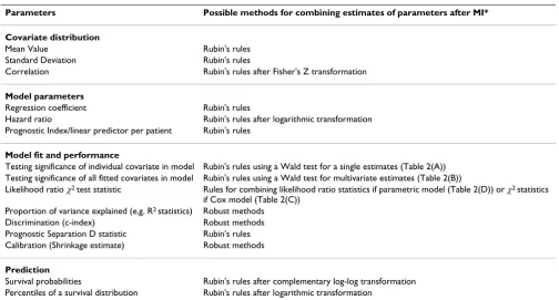
Table 1: Parameter of interest in prognostic modelling studies and ways to combine estimates after MI
Parameters Possible methods for combining estimates of parameters after MI*
Covariate distribution
Mean Value Rubin's rules
Standard Deviation Rubin's rules
Correlation Rubin's rules after Fisher's Z transformation
Model parameters
Regression coefficient Rubin's rules
Hazard ratio Rubin's rules after logarithmic transformation
Prognostic Index/linear predictor per patient Rubin's rules
Model fit and performance
Testing significance of individual covariate in model Rubin's rules using a Wald test for a single estimates (Table 2(A)) Testing significance of all fitted covariates in model Rubin's rules using a Wald test for multivariate estimates (Table 2(B))
Likelihood ratio χ2 test statistic Rules for combining likelihood ratio statistics if parametric model (Table 2(D)) or χ2 statistics
if Cox model (Table 2(C)) Proportion of variance explained (e.g. R2 statistics) Robust methods
Discrimination (c-index) Robust methods
Prognostic Separation D statistic Rubin's rules
Calibration (Shrinkage estimate) Robust methods
Prediction
Survival probabilities Rubin's rules after complementary log-log transformation
Percentiles of a survival distribution Rubin's rules after logarithmic transformation
These procedures for combining a single quantity of inter-est can be extended in matrix form to combine k estimates
of parameters, e.g. k regression coefficients, where is a k × 1 vector of these estimates and U is the associated k × k covariance matrix [4].
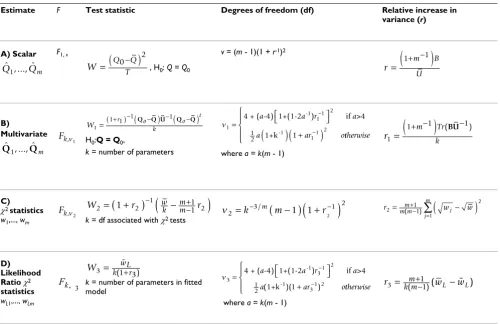
Hypothesis testing
Significance level based on a single combined estimate
A significance level for testing the null hypothesis that a single combined estimate equals a specific value, Q0: H0: Q = Q0 can be obtained using a Wald test by comparing
the test statistic against the F distribution
with one and v = (m - 1)(1 + r-1)2 degrees of freedom,
where is the relative increase in variance
due to the missing data (Table 2(A)) [4]. When the degrees of freedom, v, are close to the number of imputa-tions performed, for example with a large fraction of miss-ing information about the parameter of interest, then estimates of the parameter may be unstable and more imputations are required.
Significance level based on combined multivariate estimates
In the context of prognostic modelling, it is useful to test the global null hypothesis that all k regression estimates ˆ
Q
W =
(
Q0T−Q)
2r
m B
U =
(
1+ −)
1
Table 2: Summary of significance tests for combining different estimates from m imputed datasets after MI
Estimate F Test statistic Degrees of freedom (df) Relative increase in
variance (r)
A) Scalar F1, v
, H0: Q = Q0
v = (m - 1)(1 + r-1)2
B)
Multivariate
H0:Q = Q0,
k = number of parameters where a = k(m - 1)
C)
χ2 statistics
w1,..., wm k = df associated with χ2 tests
D) Likelihood Ratio χ2
statistics
wL1,..., wLm
k = number of parameters in fitted model
where a = k(m - 1)
KEY: F = value from the F-distribution, which the test statistic is compared to. = average of the m imputed data estimates.
= within imputation variance. B = between imputation variance.
T = total variance for the combined MI estimate.
wj, j = 1,..., m = χ2 statistics associated with testing the null hypothesis H
o : Q = Qo on each imputed dataset, such that the significance level for the jth
imputed dataset is P{ > wj}, where is the χ2 value with k degrees of freedom (Rubin 1987).
= average of the repeated χ2 statistics.
= average of the m likelihood ratio statistics, wL1,..., wLm, evaluated using the average MI parameter estimates and the average of the estimates from a model fitted subject to the null hypothesis.
ˆ ,..., ˆ
Q1 Qm W=
(
Q0T−Q)
2
r
m B
U =
(
1+ −)
1
ˆ ,..., ˆ
Q1 Qm
Fk,n1
W r o o
t
k
1
1 1 1 1
=( + )−
(
Q −Q U)
−(
Q −Q)
n111 2
11 2
2 1
= ⎡⎣ ⎤⎦
(
)
(
+)
−
−
4 + ( -4) 1+(1-2 ) if >4
1+k -1
-1
1
a a r a
a ar ottherwise
⎧ ⎨ ⎪
⎩
⎪ r m Tr
k
1
1 1 1
=
(
+ −)
−
(BU )
Fk,n2
W2=
(
1+r2)
−1(
wk −mm+−11r2)
n2 3 1
2
1 1 2
=k− /m
(
m−)
(
+r−)
r m mm wj wj m
2
2
1
1 1
= +
(
−)
−
=
∑
( )
Fk, 3
W3 k1wLr 3 = (%+ )
n3 3
1
31 2
1
2 1
= ⎡⎣ ⎤⎦
+ −
−
4 + ( -4) 1+(1-2 ) if >4
(1+k
-1 2
-1
a a r a
a )( ar ) ottherwise
⎧ ⎨ ⎪
⎩⎪ r w w
m
k m L L
3= ( +−11)( − % )
Q
U
ck2 ck2
are a specific value, zero say. A significance level for testing the hypothesis that the combined MI estimate, , equals a particular vector of values Qo is provided in Table 2(B)[9]. This ideal approach using a Wald test requires a vector of point estimates and a covariance matrix to be stored from each imputed dataset, which can be cumber-some for large k, as can result from fitting categorical var-iables in the regression model.
Significance level based on combining χ2 statistics
An alternative to testing the multivariate point estimates is the method for combining χ2 statistics, associated with testing a null hypothesis of Ho : Q = Qo, e.g. a regression coefficient is zero or all regression coefficients are zero (Table 2(C)) [8]. This approach is useful when there are a large number of parameters to estimate, the full covari-ance matrix is unobtainable from standard software or too large to store, or only the χ2 statistics are available. This approach is deficient compared to the method for com-bining multivariate estimates and should be used only as a guide, especially when there are a large number of parameters compared to only a small number of imputa-tions [22]. The true p-value lies between a half and twice this calculated value [8]. A considerable amount of infor-mation is wasted from only using the χ2 statistics and thus there is a consequent loss of power [22]. This approach may be improved by multiplying the relative increase in
variance estimate (r2 in Table 2(C)) by a factor
repre-senting the number of model parameters. Justification for this adjustment lies in the fact that each χ2 statistic is based on k degrees of freedom, but unlike the other approaches, this is not accounted for in the relative increase in variance calculations originally proposed by Li et al. [8].
Significance level based on combining likelihood ratio χ2 statistics The method for combining the likelihood ratio χ2 statis-tics [22] from each imputed dataset is used to obtain an overall significance level for testing the hypothesis of no difference between two nested prognostic models (Table 2(D)). This is an intermediate approach between combin-ing multivariate estimates and combincombin-ing χ2 statistics. The obtained significance level should be asymptotically equivalent to that based on the combined multivariate estimates [22].
The likelihood function needs to be fully specified in order to calculate the likelihood ratio statistics deter-mined at the average of the parameter estimates over the
m imputations from fitting the regression model either subject to the null hypothesis or the alternative hypothe-sis with covariates included. This may be difficult for the Cox proportional hazards model, which uses the partial likelihood function.
Guidelines for combining estimates of interest in prognostic studies
The procedures for combining multiply imputed esti-mates that are of particular interest in prognostic model-ling are discussed in the following subsections. It is assumed that the full prognostic model is fitted and its performance evaluated within each imputed dataset and the required estimates (as given in Table 1) obtained. The estimates of the parameters of interest (Table 1) are sepa-rated into those where the Rubin's rules for MI inference can be applied, those where suitable transformations can be found to improve normality and those where suitable transformations cannot be identified and therefore alter-native summary measures are proposed.
Combining estimates using Rubin's rules
The sample mean of a covariate, standard deviation, regression coefficients, individual prognostic index and the prognostic separation estimates can all be combined using Rubin's rules for single estimates. It is important to emphasise that the variance associated with a sample mean of a covariate is the sample variance divided by the number of observations and hence not just its sample var-iance [9]. The standard deviation of the data can be treated like any other parameter to give a more appropri-ate and efficient combined MI estimappropri-ate than reporting the standard deviation from only one imputed dataset. The regression coefficients, and hence the prognostic separa-tion D statistic, from fitting either a Cox proporsepara-tional haz-ards or a Weibull model should be asymptotically normal at least with large samples [15], thus making Rubin's rules appropriate.
The likelihood ratio statistic for testing the hypothesis of no difference between two nested prognostic models from each imputed dataset can be combined using the infer-ences for likelihood ratio statistics (Table 2(D)), provided that the log-likelihood function can be fully specified, e.g. for fully parametric models such as the Weibull model. The Cox proportional hazards model uses the partial like-lihood function as the baseline hazards are unspecified, and therefore can be more difficult to specify. Hence, it may be easier to use the less precise approach for combin-ing χ2 statistics (Table 2(C)). However, both these approaches are less accurate than testing the significance of the model using a Wald test based on the combined multivariate regression parameter estimates (Table 2(B)). The latter approach may be considered the preferred approach, when possible.
Q
1
Combining estimates using Rubin's rules after suitable transformation
The correlation coefficient, hazard ratios, predicted sur-vival probabilities and percentiles of the sursur-vival distribu-tion can all be combined using Rubin's rules after suitable transformations to improve normality. The obtained combined estimates should be back transformed onto their original scale prior to analysis.
Fisher's z transformation [23] provides a suitable transfor-mation for the sample correlation coefficient, which has an approximate normal distribution [9]. For large sam-ples, the log hazard ratio from a survival model, which is simply the regression coefficient, is approximately nor-mally distributed and therefore should be used. A more extreme pooled estimate than appropriate would be obtained if the hazard ratio was not transformed, as the estimates would be averaged over the posterior medians and not the posterior means as required.
The complementary log-log transformation for the pre-dicted survival probability at particular time-points gives a possible range of (-∞, +∞) instead of the survivorship estimate being bounded by zero and one, and is often used to determine reasonable confidence intervals [24]. A suitable transformation for the survival time associated with the pth percentile of a survival distribution is the log-arithmic transformation, as this gives a possible range of (-∞, +∞) instead of being bounded by zero and infinity and is generally used to obtain a confidence interval [25]. Estimates for the predicted survival probabilities at spe-cific time-points, e.g. at 2 years, or survival times at partic-ular percentiles can be obtained within each imputed dataset for the average covariate values, provided that researchers acknowledge that this does not represent the diversity of the patients in the sample [26]. Alternatively, predicted survival probabilities can be obtained for spe-cific covariate patterns or for an individual patient.
Combining model performance measures where the normality assumption is uncertain and variance estimates are generally unavailable
When considering model performance measures, the imputation model should be more general than the prog-nostic models being investigated, as the performance measures are more sensitive to the choice of imputation model and therefore may produce more bias than seen in the regression parameter estimates from the prognostic model. If one is willing to accept the large sample approx-imation to normality for the proportion of variance explained measures, e.g. Nagelkerke's R2 statistic [15], the c-index and the shrinkage estimator, then these estimates can be simply treated as another estimate that can be aver-aged using Rubin's rules for single estimates. However, estimates for these measures are generally bounded by zero and one, not symmetrically distributed and do not
necessarily follow a specific distribution, so are unlikely to follow a normal distribution. Therefore the standard MI techniques for combining into one estimate, even after applying a transformation, may not provide the best esti-mate. In addition, an overall MI variance incorporating sufficient uncertainty cannot be determined as variance estimates associated with these performance measures are generally unavailable. The lack of a within imputation variance estimate also restricts the use of sophisticated robust location and scale estimators, such as the M-esti-mators [12]. The median, inter-quartile range or full range of the m estimates may provide a more appropriate reflec-tion of the distribureflec-tion of the values over the imputed datasets, as reported by Clark and Altman [27] and Sin-haray, Stern and Russell [28] for the R2 statistics and by Clark and Altman [27] for the c-index. Using the median absolute deviation [12] could provide an alternative measure of the dispersion of values around the median.
Methods for literature review
A literature search was performed within the PubMed (National Library of Medicine) and Web of Science® bibli-ographic software of all articles published before June 2008 that used multiple imputation techniques and a sur-vival analysis to obtain a prognostic model. Methodolog-ical papers were excluded. The aim of the review was to identify how estimates of the parameters of interest in prognostic modelling studies have been combined after performing MI in the published literature.
Results
Sixteen non-methodological articles were identified. The MI techniques reported were varied with no overall con-sensus on technique or statistical software. The number of imputations ranged from five to 10000, with the majority of studies using five or ten imputations. The amount of missingness reported also varied from studies with rela-tively little missing data [29] to those with large amounts of missingness [30].
included combining percentiles from the Weibull survival distribution [36] and the median survival time and asso-ciated 95% confidence intervals from the Cox model [32] using Rubin's rules. No details of any transformations applied to these estimates prior to using Rubin's rules were reported. Gill et al. [29] and Clark et al. [30] reported model performance measures after MI, but did not explic-itly state how this was achieved after MI.
Discussion
With the advances in computer technologies and soft-ware, MI is becoming more accessible. MI has been per-formed prior to the analysis of several prognostic modelling studies, e.g. [30,31]. Few published studies explicitly stated how the reported results were obtained after MI. None of the articles identified within the current review reported that transformations were applied prior to applying Rubin's rules for any of the estimates.
This paper has suggested guidelines for combining multi-ply imputed estimates that are of interest when a survival model is fitted to a dataset and suitable performance measures and predicted survival probabilities are required for summarising the model (Table 1). These proposed guidelines are based on our own experiences and current evidence, although evidence for the appropriateness for some parameters of interest such as the mean and regres-sion coefficients are more widely available than for others such as the model performance measures. Following these guidelines can provide a more uniform approach for han-dling these estimates in future studies and hence compa-rability of reported estimates between similar studies. The standard Rubin's rules [4] should be applied to the esti-mates where the asymptotic normality assumption holds or where suitable transformations can be found. When the asymptotic normality assumption does not appear to hold or is not easily achievable, the average estimate and associated variance may be unsuitable especially with highly skewed distributions, as this could give undue weight to the tails of the distribution. Median and ranges may be more suitable, e.g. for some model performance measures, where variance estimates are generally unavail-able. More sophisticated robust estimators, such as the robust M-estimators [12], may be useful when a within imputation variance can be easily calculated. However, these robust techniques are not likelihood based, as is the case with Rubin's rules. Harel [38] showed that the pro-portion of variation explained measures, R2, from a linear regression model fitted to normally distributed data can be considered as a squared correlation coefficient and can be transformed by taking the square root and then apply-ing Fisher's Z transformation as for the correlation coeffi-cient. However whether this approach would apply to R2 measures from a survival regression model that may be affected by censored observations as arises in survival
analysis is debatable and therefore robust methods are recommended here.
In this paper, model performance measures were calcu-lated within each imputed dataset using the constructed prognostic model for that dataset and then combined to give an overall multiply imputed measure. The perform-ance of a prognostic model derived using a development sample will also need to be externally validated using an independent dataset [1], but missing data within the development and or validation sample complicate these analyses. At present there are no clear guidelines on the appropriate handling of missing data and the use of MI when externally validating a prognostic model and there-fore further research is required through the use of simu-lation studies. The extension to constructing prognostic models using variable selection procedures with multiply imputed datasets provides an added complexity, which also requires further investigation. One possible solution is to perform backwards elimination by fitting the full model in each imputed dataset and using the combined estimates to determine the least significant variable for which to exclude and then refit this reduced model. This process is continued until all non-prognostic variables have been eliminated [27]. Alternatively, bootstrapping could be incorporated [39] or a model averaging approach, as considered within the Bayesian framework [40], may also be possible.
Conclusion
The review of current practice highlighted deficiencies in the reporting of how the multiply imputed estimates given in the published articles were obtained. Thus, it is recommended that future studies include a more thor-ough description of the methods used to combine all esti-mates after MI.
The ability to use MI methods that are readily available in standard statistical software and apply simple rules to combine the estimates of interest rather than requiring problem specific programmes makes MI more accessible to practising statistician. We hope that this may lead to a more widespread and appropriate use of MI in future prognostic modelling studies and improved comparabil-ity of the obtained estimates between studies.
Abbreviations
MI: multiple imputation; m: number of imputations; SE: standard error.
Competing interests
The authors declare that they have no competing interests.
Authors' contributions
con-ception of this research, the methodological content, the design, coordination and analysis of the literature review and drafted the manuscript. DGA was involved in the con-ception and design of the study and helped in the writing of the manuscript. RLH participated in the design and methodological content of this study and in the revision of the manuscript. PR contributed to the methodological content of this research and the revision of the manu-script. All authors have read and approved the final man-uscript.
Acknowledgements
Andrea Marshall (nee Burton) was supported by a Cancer Research UK project grant. DGA is supported by Cancer Research UK.
References
1. Altman DG, Royston P: What do we mean by validating a prog-nostic model? Statistics in Medicine 2000, 19(4):453-473. 2. Wyatt JC, Altman DG: Commentary: Prognostic models:
clini-cally useful or quickly forgotten? British Medical Journal 1995, 311(7019):1539-1541.
3. Burton A, Altman DG: Missing covariate data within cancer prognostic studies: a review of current reporting and pro-posed guidelines. British Journal of Cancer 2004, 91(1):4-8. 4. Rubin DB: Multiple Imputation for Nonresponse in Surveys New York:
John Wiley and Sons; 2004.
5. Graham JW, Olchowski AE, Gilreath TD: How many imputations are really needed? Some practical clarifications of multiple imputation theory. Prevention Science 2007, 8(3):206-213. 6. Kenward MG, Carpenter J: Multiple imputation: current
per-spectives. Statistical Methods in Medical Research 2007, 16(3):199-218.
7. van Buuren S, Boshuizen HC, Knook DL: Multiple imputation of missing blood pressure covariates in survival analysis. Statis-tics in Medicine 1999, 18(6):681-694.
8. Li KH, Meng XL, Raghunathan TE, Rubin DB: Significance levels from repeated p-values with multiply-imputed data. Statistica Sinica 1991, 1(1):65-92.
9. Schafer JL: Analysis of Incomplete Multivariate Data New York: Chap-man and Hall; 1997.
10. Rubin DB, Schenker N: Multiple imputation in health-care data-bases: an overview and some applications. Statistics in Medicine 1991, 10(4):585-598.
11. Rubin DB, Schenker N: Multiple imputation for interval estima-tion from simple random samples with ignorable nonre-sponse. Journal of the American Statistical Association 1986, 81(394):366-374.
12. Hampel FR, Ronchetti EM, Rousseeuw PJ, Stahel WA: Robust statistics. The approach based on influence functions New York: John Wiley & Sons; 1986.
13. Ambler G, Brady AR, Royston P: Simplifying a prognostic model: a simulation study based on clinical data. Statistics in Medicine 2002, 21(24):3803-3822.
14. Peduzzi P, Concato J, Feinstein AR, Holford TR: Importance of events per independent variable in proportional hazards regression analysis. II. Accuracy and precision of regression estimates. Journal of Clinical Epidemiology 1995, 48(12):1503-1510. 15. Harrell FE: Regression Modeling Strategies with Applications to Linear
Models, Logistic Regression, and Survival Analysis New York: Springer-Verlag; 2001.
16. Schemper M, Stare J: Explained variation in survival analysis.
Statistics in Medicine 1996, 15(19):1999-2012.
17. Schemper M, Henderson R: Predictive accuracy and explained variation in Cox regression. Biometrics 2000, 56(1):249-255. 18. O'Quigley J, Xu RH, Stare J: Explained randomness in
propor-tional hazards models. Statistics in Medicine 2005, 24(3):479-489. 19. Harrell FE, Lee KL, Mark DB: Multivariable prognostic models: issues in developing models, evaluating assumptions and adequacy, and measuring and reducing errors. Statistics in Medicine 1996, 15(4):361-387.
20. Royston P, Sauerbrei W: A new measure of prognostic separa-tion in survival data. Statistics in Medicine 2004, 23(5):723-748. 21. van Houwelingen HC, Le Cessie S: Predictive value of statistical
models. Statistics in Medicine 1990, 9(1):1303-1325.
22. Meng XL, Rubin DB: Performing likelihood ratio tests with multiply-imputed data sets. Biometrika 1992, 79(1):103-111. 23. Fisher RA: Statistical Methods for Research Workers Edinburgh: Oliver
and Boyd Ltd; 1941.
24. Hosmer DW, Lemeshow S: Applied survival analysis – Regression mode-ling of time to event data New York: John Wiley & Sons; 1999. 25. Collett D: Modelling survival data in medical research Second edition.
London: Chapman & Hall/CRC; 2003.
26. Thomsen BL, Keiding N, Altman DG: A note on the calculation of expected survival, illustrated by the survival of liver trans-plant patients. Statistics in Medicine 1991, 10(5):733-738. 27. Clark TG, Altman DG: Developing a prognostic model in the
presence of missing data. an ovarian cancer case study. Jour-nal of Clinical Epidemiology 2003, 56(1):28-37.
28. Sinharay S, Stern HS, Russell D: The use of multiple imputation for the analysis of missing data. Psychological Methods 2001, 6(4):317-329.
29. Gill S, Loprinzi CL, Sargent DJ, Thome SD, Alberts SR, Haller DG, Benedetti J, Francini G, Shepherd LE, Seitz JF, et al.: Pooled analysis of fluorouracil-based adjuvant therapy for stage II and III colon cancer: Who benefits and by how much? Journal of Clini-cal Oncology 2004, 22(10):1797-1806.
30. Clark TG, Stewart ME, Altman DG, Gabra H, Smyth JF: A prognos-tic model for ovarian cancer. British Journal of Cancer 2001, 85(7):944-952.
31. Rouxel A, Hejblum G, Bernier MO, Boelle PY, Menegaux F, Mansour G, Hoang C, Aurengo A, Leenhardt L: Prognostic factors associ-ated with the survival of patients developing loco-regional recurrences of differentiated thyroid carcinomas. J Clin Endo-crinol Metab 2004, 89(11):5362-5368.
32. Stadler WM, Huo DZ, George C, Yang XM, Ryan CW, Karrison T, Zim-merman TM, Vogelzang NJ: Prognostic factors for survival with gemcitabine plus 5-fluorouracil based regimens for metastatic renal cancer. Journal of Urology 2003, 170(4):1141-1145.
33. Vaughn G, Detels R: Protease inhibitors and cardiovascular dis-ease: analysis of the Los Angeles County adult spectrum of disease cohort. AIDS Care 2007, 19(4):492-499.
34. Orsini N, Mantzoros CS, Wolk A: Association of physical activity with cancer incidence, mortality, and survival: a population-based study of men. British Journal of Cancer 2008, 98(11):1864-1869. 35. Mertens AC, Yasui Y, Neglia JP, Potter JD, Nesbit ME, Ruccione K, Smithson WA, Robison LL: Late mortality experience in five-year survivors of childhood and adolescent cancer: The child-hood cancer survivor study. Journal of Clinical Oncology 2001, 19(13):3163-3172.
36. Serrat C, Gomez G, de Olalla PG, Cayla JA: CD4+ lymphocytes and tuberculin skin test as survival predictors in pulmonary tuberculosis HIV-infected patients. International Journal of Epide-miology 1998, 27(4):703-712.
37. Bärnighausen T, Tanser F, Gqwede Z, Mbizana C, Herbst K, Newell M-L: High HIV incidence in a community with high HIV prev-alence in rural South Africa: findings from a prospective pop-ulation-based study. AIDS 2008, 22(1):139-144.
38. Harel O: The estimation of R^2 and adjusted R^2 in incom-plete data sets using multiple imputation. Journal of Applied Sta-tistics 2009 in press. http://www.informaworld.com/10.1080/ 02664760802553000
39. Heymans MW, van Buuren S, Knol DL, van Mechelen W, de Vet HCW: Variable selection under multiple imputation using the bootstrap in a prognostic study. BMC Medical Research Meth-odology 2007, 7:33.
40. Hoeting JA, Madigan D, Raftery AE, Volinsky CT: Bayesian model averaging: A tutorial. Statistical Science 1999, 14(4):382-401.
Pre-publication history
The pre-publication history for this paper can be accessed here: