98
Chapter
S
hown here is the pain reliever acetamino-
phen in crystalline form, photographed
under a transmitted light microscope. While
acetaminophen relieves pain with few side effects,
it is toxic in large doses. One study found that only
30% of parents who gave acetaminophen to their
children could accurately calculate and measure
the correct dose.
One rule for calculating the dosage (mg) of
acetaminophen for children ages 1 to 12 years old
is D
(
t
)
750
t
(
t
12),
where t
is age in years.
What is an expression for the rate of change of a
child’s dosage with respect to the child’s age? How
does the rate of change of the dosage relate to
the growth rate of children? This problem can be
solved with the information covered in Section 3.4.
Derivatives
Chapter 3 Overview
In Chapter 2, we learned how to find the slope of a tangent to a curve as the limit of the
slopes of secant lines. In Example 4 of Section 2.4, we derived a formula for the slope of
the tangent at an arbitrary point
a
, 1
a
on the graph of the function
f
x
1
x
and
showed that it was
1
a
2.
This seemingly unimportant result is more powerful than it might appear at first glance,
as it gives us a simple way to calculate the instantaneous rate of change of
f
at any point.
The study of rates of change of functions is called
differential calculus,
and the formula
1
a
2was our first look at a
derivative.
The derivative was the 17th-century breakthrough
that enabled mathematicians to unlock the secrets of planetary motion and gravitational
attraction— of objects changing position over time. We will learn many uses for
deriva-tives in Chapter 4, but first we will concentrate in this chapter on understanding what
de-rivatives are and how they work.
Derivative of a Function
Definition of Derivative
In Section 2.4, we defined the slope of a curve
y
f
x
at the point where
x
a
to be
m
lim
h→0
f
a
h
h
f
a
.
When it exists, this limit is called the
derivative of
f
at
a.
In this section, we investigate
the derivative as a
function
derived from
f
by considering the limit at each point of the
do-main of
f.
3.1
What you’ll learn about
• Definition of Derivative
• Notation
• Relationships between the
Graphs of
f
and
f
• Graphing the Derivative from
Data
• One-sided Derivatives
. . . and why
The derivative gives the value of
the slope of the tangent line to a
curve at a point.
DEFINITION
Derivative
The
derivative
of the function
f
with respect to the variable
x
is the function
f
whose value at
x
is
f
x
lim
h→0
f
x
h
h
f
x
,
(1)
provided the limit exists.
continued
The domain of
f
, the set of points in the domain of
f
for which the limit exists, may be
smaller than the domain of
f.
If
f
x
exists, we say that
f
has a derivative (is
differen-tiable)
at
x.
A function that is differentiable at every point of its domain is a
differentiable
function.
SOLUTION
Applying the definition, we have
f
x
lim
h→0
f
x
h
h
f
x
lim
h→0
x
h
h
3x
3lim
h→0
lim
h→0
3
x
23
x
h
h
h
2h
lim
h→0
3
x
2
3
xh
h
23
x
2.
Now try Exercise 1.The derivative of
f
x
at a point where
x
a
is found by taking the limit as
h
→
0 of
slopes of secant lines, as shown in Figure 3.1.
By relabeling the picture as in Figure 3.2, we arrive at a useful alternate formula for
calculating the derivative. This time, the limit is taken as
x
approaches
a.
x
33
x
2h
3
xh
2h
3x
3h
xh3 expanded
x3s cancelled,
h factored out
After we find the derivative of
f
at a point
x
a
using the alternate form, we can find
the derivative of
f
as a function by applying the resulting formula to an arbitrary
x
in the
domain of
f.
EXAMPLE 2
Applying the Alternate Definition
Differentiate
f
x
x
using the alternate definition.
SOLUTION
At the point
x
a
,
f
a
lim
x→a
f
x
x
a
f
a
lim
x→a
x
x
a
a
Eq. 2 with fx
lim
x→a
x
x
a
a
•
x
x
a
a
Rationalize…
lim
x→a …the numerator.
lim
x→a
x
1
a
We can now take the limit.2
1
a
.
Applying this formula to an arbitrary
x
0 in the domain of
f
identifies the derivative as
the function
f
x
1
2
x
with domain
0,
.
Now try Exercise 5.x
a
x
a
x
a
1x x
y
f(a + h)
f(a) P(a, f(a))
Q(a + h, f(a + h))
y = f(x)
x
y
a a + h O
Figure 3.1 The slope of the secant line
PQis
yx faahhfaa
fah h
fa
.
x y
f(x)
f(a) P(a, f(a))
Q(x, f(x))
y = f(x)
x
y
a x
O
Figure 3.2 The slope of the secant line
PQis
y x
fx x
a fa
.
DEFINITION (ALTERNATE)
Derivative at a Point
The
derivative
of the function
f
at the point
x
a
is the limit
f
a
lim
x→a
f
x
x
a
f
a
,
(2)
provided the limit exists.
Eq. 1 with fx x3,
Notation
There are many ways to denote the derivative of a function
y
f
x
. Besides
f
x
, the
most common notations are these:
y
“
y
prime”
Nice and brief, but does not name
the independent variable.
“
dy dx
” or “the derivative
Names both variables and
of
y
with respect to
x
”
uses
d
for derivative.
“
df dx
” or “the derivative
Emphasizes the function’s name.
of
f
with respect to
x
”
f
x
“
d dx
of
f
at
x
” or “the
Emphasizes the idea that
differentia-derivative of
f
at
x
”
tion is an operation performed on
f.
Relationships between the Graphs of
f
and
f
When we have the explicit formula for
f
x
, we can derive a formula for
f
x
using
meth-ods like those in Examples 1 and 2. We have already seen, however, that functions are
en-countered in other ways: graphically, for example, or in tables of data.
Because we can think of the derivative at a point in graphical terms as
slope,
we can get
a good idea of what the graph of the function
f
looks like by
estimating the slopes
at
var-ious points along the graph of
f.
EXAMPLE 3
GRAPHING f
from f
Graph the derivative of the function
f
whose graph is shown in Figure 3.3a. Discuss the
behavior of
f
in terms of the signs and values of
f
.
d
dx
df
dx
dy
dx
Why all the notation?
The “prime” notations yand fcome from notations that Newton used for derivatives. Theddxnotations are similar to those used by Leibniz. Each has its advantages and disadvantages.
x y
2
A
B C
D
E F
4 5
3
–1
1 2
(a)
3 5 6 7
y = f(x)
Slope 4 Slope 1
Slope 0
Slope 0 Slope –1
Slope –1
4 x
y'
2
1 3
A'
B'
C'
D'
(b)
E' F'
4
–1
1 2 3 5 6 7
y' = f'(x) (slope)
4 5
Figure 3.3 By plotting the slopes at points on the graph of yfx, we obtain a graph of
y fx. The slope at point Aof the graph offin part (a) is the y-coordinate of point Aon the graph offin part (b), and so on. ( Example 3)
SOLUTION
First, we draw a pair of coordinate axes, marking the horizontal axis in
x
-units and the
vertical axis in slope units ( Figure 3.3b). Next, we estimate the slope of the graph of
f
at various points, plotting the corresponding slope values using the new axes. At
A
0,
f
0
, the graph of
f
has slope 4, so
f
0
4. At
B
, the graph of
f
has slope 1,
so
f
1 at
B
, and so on.
We complete our estimate of the graph of
f
by connecting the plotted points with a
smooth curve.
Although we do not have a formula for either
f
or
f
, the graph of each reveals important
information about the behavior of the other. In particular, notice that
f
is decreasing
where
f
is negative and increasing where
f
is positive. Where
f
is zero, the graph of
f
has a horizontal tangent, changing from increasing to decreasing (point
C
) or from
decreasing to increasing (point
F
).
Now try Exercise 23.Reading the Graphs
Suppose that the function
f
in Figure 3.3a represents the depth
y
(in inches) of water
in a ditch alongside a dirt road as a function of time
x
(in days). How would you
an-swer the following questions?
1.
What does the graph in Figure 3.3b represent? What units would you use along
the
y
-axis?
2.
Describe as carefully as you can what happened to the water in the ditch over
the course of the 7-day period.
3.
Can you describe the weather during the 7 days? When was it the wettest?
When was it the driest?
4.
How does the graph of the derivative help in finding when the weather was
wettest or driest?
5.
Interpret the significance of point
C
in terms of the water in the ditch. How does
the significance of point
C
reflect that in terms of rate of change?
6.
It is tempting to say that it rains right up until the beginning of the second day,
but that overlooks a fact about rainwater that is important in flood control.
Explain.
Construct your own “real-world” scenario for the function in Example 3, and pose
a similar set of questions that could be answered by considering the two graphs in
Figure 3.3.
EXPLORATION 1
x y
2
–2
2 –2
y = f(x)
x y
2
–2
2 –2
y = f(x)
Figure 3.4 The graph of the derivative. ( Example 4)
Figure 3.5 The graph off, constructed from the graph offand two other conditions. ( Example 4)
EXAMPLE 4
Graphing
f
from
f
Sketch the graph of a function
f
that has the following properties:
i.
f
0
0;
ii.
the graph of
f
, the derivative of
f
, is as shown in Figure 3.4;
iii.
f
is continuous for all
x.
SOLUTION
To satisfy property (i), we begin with a point at the origin.
To satisfy property (ii), we consider what the graph of the derivative tells us about slopes.
To the left of
x
1, the graph of
f
has a constant slope of
1; therefore we draw a line
with slope
1 to the left of
x
1, making sure that it goes through the origin.
To the right of
x
1, the graph of
f
has a constant slope of 2, so it must be a line with
slope 2. There are infinitely many such lines but only one—the one that meets the left
side of the graph at
1,
1
—will satisfy the continuity requirement. The resulting
Graphing the Derivative from Data
Discrete points plotted from sets of data do not yield a continuous curve, but we have seen
that the shape and pattern of the graphed points (called a scatter plot) can be meaningful
nonetheless. It is often possible to fit a curve to the points using regression techniques. If
the fit is good, we could use the curve to get a graph of the derivative visually, as in
Exam-ple 3. However, it is also possible to get a scatter plot of the derivative numerically,
di-rectly from the data, by computing the slopes between successive points, as in Example 5.
EXAMPLE 5
Estimating the Probability of Shared Birthdays
Suppose 30 people are in a room. What is the probability that two of them share the
same birthday? Ignore the year of birth.
SOLUTION
It may surprise you to learn that the probability of a shared birthday among 30 people is at
least 0.706, well above two-thirds! In fact, if we assume that no one day is more likely to
be a birthday than any other day, the probabilities shown in Table 3.1 are not hard to
deter-mine (see Exercise 45).
Table 3.1 Probabilities of Shared Birthdays
People in
Room x Probability y
0 0
5 0.027 10 0.117 15 0.253 20 0.411 25 0.569 30 0.706 35 0.814 40 0.891 45 0.941 50 0.970 55 0.986 60 0.994 65 0.998 70 0.999
Table 3.2 Estimates of Slopes on the Probability Curve
Midpoint of Change Interval x slope y
x2.5 0.0054 7.5 0.0180 12.5 0.0272 17.5 0.0316 22.5 0.0316 27.5 0.0274 32.5 0.0216 37.5 0.0154 42.5 0.0100 47.5 0.0058 52.5 0.0032 57.5 0.0016 62.5 0.0008 67.5 0.0002
A scatter plot of the data in Table 3.1 is shown in Figure 3.6.
Notice that the probabilities grow slowly at first, then faster, then much more slowly
past
x
45. At which
x
are they growing the fastest? To answer the question, we need
the graph of the derivative.
Using the data in Table 3.1, we compute the slopes between successive points on the
proba-bility plot. For example, from
x
0 to
x
5 the slope is
0.0
5
2
7
0
0
0.0054.
We make a new table showing the slopes, beginning with slope 0.0054 on the interval
0, 5
( Table 3.2). A logical
x
value to use to represent the interval is its midpoint 2.5.
continued
David H. Blackwell
(1919–
)
By the age of 22, David Blackwell had earned a Ph.D. in Mathematics from the University of Illinois. He taught at Howard University, where his research included sta-tistics, Markov chains, and sequential analysis. He then went on to teach and continue his research at the University of California at Berkeley. Dr. Blackwell served as president of the American Statistical Association and was the first African American mathematician of the National Academy of Sciences.
[–5, 75] by [–0.2, 1.1]
5
1
Figure 3.6 Scatter plot of the probabili-ties yof shared birthdays among x peo-ple, for x0, 5, 10, . . . , 70. ( Example 5)
What’s happening at x1?
Notice that fin Figure 3.5 is defined at
x1, while fis not. It is the continuity of fthat enables us to conclude that
A scatter plot of the derivative data in Table 3.2 is shown in Figure 3.7.
From the derivative plot, we can see that the rate of change peaks near
x
20. You can
impress your friends with your “psychic powers” by predicting a shared birthday in a
room of just 25 people (since you will be right about 57% of the time), but the derivative
warns you to be cautious: a few less people can make quite a difference. On the other
hand, going from 40 people to 100 people will not improve your chances much at all.
Now try Exercise 29.
Generating shared birthday probabilities:
If you know a little about probability, you
might try generating the probabilities in Table 3.1. Extending the Idea Exercise 45 at the
end of this section shows how to generate them on a calculator.
One-Sided Derivatives
A function
y
f
x
is
differentiable on a closed interval
a
,
b
if it has a derivative at
every interior point of the interval, and if the limits
lim
h→0
f
a
h
h
f
a
[the
right-hand derivative at
a
]
lim
h→0
f
b
h
h
f
b
[the
left-hand derivative at
b
]
exist at the endpoints. In the right-hand derivative,
h
is positive and
a
h
approaches
a
from
the right. In the left-hand derivative,
h
is negative and
b
h
approaches
b
from the left
(Figure 3.8).
Right-hand and left-hand derivatives may be defined at any point of a function’s
domain.
The usual relationship between one-sided and two-sided limits holds for derivatives.
Theorem 3, Section 2.1, allows us to conclude that a function has a (two-sided) derivative
at a point if and only if the function’s right-hand and left-hand derivatives are defined and
equal at that point.
EXAMPLE 6
One-Sided Derivatives can Differ at a Point
Show that the following function has left-hand and right-hand derivatives at
x
0, but
no derivative there ( Figure 3.9).
x
2,
x
0
y
{
2
x
,
x
0
SOLUTION
We verify the existence of the left-hand derivative:
lim
h→0
0
h
h
20
2lim
h→0
h
h
2
0.
We verify the existence of the right-hand derivative:
lim
h→0
hlim
→02
h
h
2.
Since the left-hand derivative equals zero and the right-hand derivative equals 2, the
de-rivatives are not equal at
x
0. The function does not have a derivative at 0.
Now try Exercise 31.
2
0
h
0
2h
x yf(x)
a ah bh b h 0 h 0
Slope lim
h 0–
f(bh) f(b) ———————
h
Slope lim
h 0+
f(ah) f(a) ———————
h
x y
2
1 1
–1
–1
Figure 3.8 Derivatives at endpoints are one-sided limits.
Figure 3.7 A scatter plot of the deriva-tive data in Table 3.2. ( Example 5)
[–5, 75] by [–0.01, 0.04]
20
40
60
In Exercises 1–4, evaluate the indicated limit algebraically.
1.lim
h→0
2h h
24
4 2. lim
x→2
x
2 3
5/2
3.lim
y→0 1 4.xlim→4
2x x
8
2
8
5.Find the slope of the line tangent to the parabola yx21
at its vertex. 0
6.By considering the graph of fxx33x22, find the
intervals on whichfis increasing. ( , 0] and [2, )
y
y
Quick Review 3.1
(For help, go to Sections 2.1 and 2.4.)
In Exercises 7–10, let
x2, x1
fx
{
x12, x1.
7. Find limx→1fx and limx→1fx.
8. Find limh→0f1h. 0
9. Does limx→1fx exist? Explain. No, the two one-sided limits
10.Isfcontinuous? Explain. No,fis discontinuous at x1 because the limit doesn’t exist there.
Section 3.1 Exercises
In Exercises 1–4, use the definition
fa lim
h→0
f(ah h
)f(a)
to find the derivative of the given function at the indicated point.
1.f(x)1x,a 2 1
4 2. f(x)x24,a1 23.f(x)3x2,a 1 2 4. f(x)x3x,a0 1
In Exercises 5–8, use the definition
f(a) lim
x→a
f(x x
)
f a
(a)
to find the derivative of the given function at the indicated point.
5.f(x)1x,a2 1
4 6. f(x)x24,a1 27.f(x)x1,a3 1
4 8. f(x)2x3,a 1 29. Find fxif fx3x12. f(x) 3
10.Find dy
dx if y7x. dy/dx 711.Find
d d
x
x2. 2x
12.Find f(x) if f(x)3x2. 6x
In Exercises 13–16, match the graph of the function with the graph of the derivative shown here:
d dx
13.
14.
15.
16.
17.If f23 and f25, find an equation of (a)the tangent
line,and (b)the normal line to the graph of yfx at the point where x 2.
y
O x
yf4(x)
y
O x
yf3(x)
x y
O
yf2(x)
x y
O
yf1(x)
y'
O x
(a)
y'
O x
(b)
y'
O x
(c)
y'
O x
(d)
lim
x→1f(x) 0 ; limx→1 f(x) 3
are different.
(b)
(a)
(d)
(c)
(a)y5x7
(b) y 1
5x 1
5 7
18.Find the derivative of the function y2x213x5 and use it
to find an equation of the line tangent to the curve at x3. 19.Find the lines that are (a)tangent and (b)normal to the curve
yx3at the point 1, 1. (a)y3x2 (b)y 1
3x 4 3
20.Find the lines that are (a)tangent and (b)normal to the curve
yxat x4.
21.Daylight in Fairbanks The viewing window below shows the number of hours of daylight in Fairbanks, Alaska, on each day for a typical 365-day period from January 1 to December 31. Answer the following questions by estimating slopes on the graph in hours per day. For the purposes of estimation, assume that each month has 30 days.
(a)On about what date is the amount of daylight increasing at the fastest rate? What is that rate?
(b)Do there appear to be days on which the rate of change in the amount of daylight is zero? If so, which ones? Yes. Jan. 1 and
(c)On what dates is the rate of change in the number of daylight hours positive? negative? Positive: Jan 1, through July 1
22.Graphing ffrom f Given the graph of the functionfbelow, sketch a graph of the derivativeoff.
23.The graphs in Figure 3.10a show the numbers of rabbits and foxes in a small arctic population. They are plotted as functions of time for 200 days. The number of rabbits increases at first, as the rabbits reproduce. But the foxes prey on the rabbits and, as the number of foxes increases, the rabbit population levels off and then drops. Figure 3.10b shows the graph of the derivative of the rabbit population. We made it by plotting slopes, as in Example 3.
(a)What is the value of the derivative of the rabbit population in Figure 3.10 when the number of rabbits is largest? smallest?
(b)What is the size of the rabbit population in Figure 3.10 when its derivative is largest? smallest? 1700 and 1300
[–5, 5] by [–3, 3] [0, 365] by [0, 24]
24.Shown below is the graph of fxxlnxx. From what you know about the graphs of functions (i) through (v), pick out the one that is the derivativeofffor x0. (ii)
i.ysinx ii.ylnx iii.yx iv.yx2 v.y3x1
25.From what you know about the graphs of functions (i) through (v), pick out the one that is its own derivative. (iv)
i.ysinx ii.yx iii.yx iv.yex v.yx2
[–2, 6] by [–3, 3] Number
of rabbits
Initial no. rabbits 1000 Initial no. foxes 40
Number of foxes
(20, 1700)
0 50 100 150 200
0 1000 2000
Time (days) (a)
(20, 40)
0 50 100 150 200
100
50 50
Time (days)
Derivative of the rabbit population
100
0
(b)
Figure 3.10 Rabbits and foxes in an arctic predator-prey food chain.Source: Differentiation by W. U. Walton et al., Project CALC, Education Development Center, Inc., Newton, MA, 1975, p. 86.
4
Sometime around April 1. The rate then is approximately 1/6 hour per day.
July 1
Negative: July 1 through Dec. 31
0 and 0
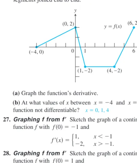
26.The graph of the function yfx shown here is made of line segments joined end to end.
(a)Graph the function’s derivative.
(b)At what values of xbetween x 4 and x6 is the function not differentiable? x0, 1, 4
27.Graphing f from f Sketch the graph of a continuous functionfwith f0 1 and
1, x 1
fx
{
2, x 1.
28. Graphing f from f Sketch the graph of a continuous functionfwith f01 and
2, x2
fx
{
1, x2.
In Exercises 29 and 30, use the data to answer the questions.
29.A Downhill Skier Table 3.3 gives the approximate distance traveled by a downhill skier after tseconds for 0t10. Use the method of Example 5 to sketch a graph of the derivative; then answer the following questions:
(a)What does the derivative represent? The speed of the skier
(b)In what units would the derivative be measured?
(c)Can you guess an equation of the derivative by considering its graph? Approximately D= 6.65t
30.A Whitewater River Bear Creek, a Georgia river known to kayaking enthusiasts, drops more than 770 feet over one stretch of 3.24 miles. By reading a contour map, one can estimate the
x y
0
y f(x)
1
(– 4, 0) 6
(0, 2) (6, 2)
(4, – 2) (1, – 2)
elevations yat various distances xdownriver from the start of the kayaking route ( Table 3.4).
(a) Sketch a graph of elevation yas a function of distance downriver x.
(b)Use the technique of Example 5 to get an approximate graph of the derivative,dy
dx.(c) The average change in elevation over a given distance is called a gradient. In this problem, what units of measure would be appropriate for a gradient? Feet per mile
(d)In this problem, what units of measure would be appropriate for the derivative? Feet per mile
(e) How would you identify the most dangerous section of the river (ignoring rocks) by analyzing the graph in (a)? Explain.
(f)How would you identify the most dangerous section of the river by analyzing the graph in (b)? Explain.
31.Using one-sided derivatives, show that the function
x2 x, x1
fx
{
3x 2, x1 does not have a derivative at x1.
32.Using one-sided derivatives, show that the function
x3, x1
fx
{
3x, x1 does not have a derivative at x1.
33.Writing to Learn Graph ysinxand ycosxin the same viewing window. Which function could be the derivative of the other? Defend your answer in terms of the behavior of the graphs.
34.In Example 2 of this section we showed that the derivative of
yx is a function with domain 0, . However, the function yx itself has domain 0, , so it could have a right-hand derivative at x0. Prove that it does not. 35.Writing to Learn Use the concept of the derivative to define
[image:10.684.50.278.77.346.2]what it might mean for two parabolas to be parallel. Construct equations for two such parallel parabolas and graph them. Are the parabolas “everywhere equidistant,” and if so, in what sense?
Table 3.3 Skiing Distances Time t Distance Traveled (seconds) (feet)
0 0
1 3.3
2 13.3
3 29.9
4 53.2
5 83.2
6 119.8
7 163.0
8 212.9
9 269.5
10 332.7
Table 3.4 Elevations along Bear Creek Distance Downriver River Elevation
(miles) (feet)
0.00 1577
0.56 1512
0.92 1448
1.19 1384
1.30 1319
1.39 1255
1.57 1191
1.74 1126
1.98 1062
2.18 998
2.41 933
2.64 869
3.24 805
Standardized Test Questions
You should solve the following problems without using a graphing calculator.
36.True or False If f(x)x2x, then f(x) exists for every real
number x. Justify your answer. True.f(x)2x1
37.True or False If the left-hand derivative and the right-hand derivative of fexist at xa, then f(a) exists. Justify your answer.
38.Multiple Choice Let f(x)43x. Which of the following is equal to f(1)? C
(A)7 (B)7 (C)3 (D)3 (E)does not exist
39.Multiple Choice Let f(x)13x2. Which of the following
is equal to f(1)? A
(A)6 (B)5 (C)5 (D)6 (E)does not exist
In Exercises 40 and 41, let
x2 1, x0
fx
{
2x 1, x0.
40.Multiple Choice Which of the following is equal to the left-hand derivative of f at x0? B
(A)2 (B)0 (C)2 (D) (E)
41.Multiple Choice Which of the following is equal to the right-hand derivative of f at x0? C
(A)2 (B)0 (C)2 (D) (E)
Explorations
42. x
2, x1
Letfx
{
2x, x1.
(a)Find fx for x 1. 2x (b)Find fx for x1. (c)Find limx→1fx. 2 (d)Find limx→1fx. 2
(e)Does limx→1fx exist? Explain. Yes, the two one-sided
(f)Use the definition to find the left-hand derivative off
at x1 if it exists. 2
(g)Use the definition to find the right-hand derivative off
at x1 if it exists. Does not exist
(h)Does f1 exist? Explain. It does not exist because the
right-43.Group Activity Using graphing calculators, have each person in your group do the following:
(a)pick two numbers aand bbetween 1 and 10; (b)graph the function yxaxb;
(c)graph the derivativeof your function (it will be a line with slope 2);
(d)find the y-intercept of your derivative graph.
(e)Compare your answers and determine a simple way to predict the y-intercept, given the values of aand b.Test your result.
Extending the Ideas
44. Find the unique value of kthat makes the function
x3, x1
fx
{
3xk, x1 differentiable at x1. k 2
45.Generating the Birthday Probabilities Example 5 of this section concerns the probability that, in a group of npeople, at least two people will share a common birthday. You can generate these probabilities on your calculator for values of n
from 1 to 365.
Step 1: Set the values of N and P to zero:
Step 2: Type in this single, multi-step command:
Now each time you press the ENTER key, the command will print a new value of N (the number of people in the room) alongside P (the probability that at least two of them share a common birthday):
If you have some experience with probability, try to answer the following questions without looking at the table:
(a)If there are three people in the room, what is the probability that they all have differentbirthdays? (Assume that there are 365 possible birthdays, all of them equally likely.) 0.992
(b)If there are three people in the room, what is the probability that at least two of them share a common birthday? 0.008
(c)Explain how you can use the answer in part (b) to find the probability of a shared birthday when there are fourpeople in the room. ( This is how the calculator statement in Step 2 generates the probabilities.)
(d)Is it reasonable to assume that all calendar dates are equally likely birthdays? Explain your answer.
.0082041659}
.0163559125}
.0271355737}
.0404624836}
.0562357031}
{2
{3
{4
{5
{6
{7
{1 0}
.002739726}
N+1 N: 1–(1–P) (366
–N)/365 P: {N,P}
0 N:0 P
0
False. Letf(x)⏐x⏐. The left hand derivative atx0 is1 and the right hand derivative atx0 is 1.f(0) does not exist.
2
limits exist and are the same.
hand derivative does not exist.
The y-intercept is ba.
(c)If Pis the answer to (b), then the probability of a shared birthday when there are four people is
1(1 P) 3 3
6 6 2 5
Differentiability
How
f
(
a
) Might Fail to Exist
A function will not have a derivative at a point
P
a
,
f
a
where the slopes of the secant lines,
f
x
x
a
f
a
,
fail to approach a limit as
x
approaches
a.
Figures 3.11–3.14 illustrate four different
in-stances where this occurs. For example, a function whose graph is otherwise smooth will
fail to have a derivative at a point where the graph has
1.
a
corner,
where the one-sided derivatives differ; Example:
f
x
x
3.2
What you’ll learn about
• How
f
(
a
) Might Fail to Exist
• Differentiability Implies Local
Linearity
• Derivatives on a Calculator
• Differentiability Implies
Continuity
• Intermediate Value Theorem
for Derivatives
. . . and why
Graphs of differentiable functions
can be approximated by their
tangent lines at points where the
derivative exists.
[–3, 3] by [–2, 2] [–3, 3] by [–2, 2]
Figure 3.11 There is a “corner” at x0. Figure 3.12 There is a “cusp” at x0.
2.
a
cusp,
where the slopes of the secant lines approach
from one side and
from
the other (an extreme case of a corner); Example:
f
x
x
233.
a
vertical tangent,
where the slopes of the secant lines approach either
or
from
both sides (in this example,
); Example:
f
x
3x
4.
a
discontinuity
(which will cause one or both of the one-sided derivatives to be
non-existent). Example: The
Unit Step Function
In this example, the left-hand derivative fails to exist:
lim
h→0
1
h
1
lim
h→0
h
2
.
1,
x
0
U
x
{
1,
x
0
[–3, 3] by [–2, 2]
Figure 3.13 There is a vertical tangent line at x0.
Figure 3.14 There is a discontinuity at x0.
[–3, 3] by [–2, 2]
How rough can the graph of a continuous function be?
The graph of the absolute value function fails to be differentiable at a single point. If you graph ysin1 (sin (x)) on
your calculator, you will see a continu-ous function with an infinitenumber of points of nondifferentiability. But can a continuous function fail to be differen-tiable at everypoint?
The answer, surprisingly enough, is yes, as Karl Weierstrass showed in 1872. One of his formulas (there are many like it) was
fx
∞
n0
2
3
n
cos9nx,
Later in this section we will prove a theorem that states that a function
must
be
contin-uous at
a
to be differentiable at
a.
This theorem would provide a quick and easy
verifica-tion that
U
is not differentiable at
x
0.
EXAMPLE 1
Finding Where a Function is not Differentiable
Find all points in the domain of
f
x
x
2
3 where
f
is not differentiable.
SOLUTION
Think graphically! The graph of this function is the same as that of
y
x
, translated 2
units to the right and 3 units up. This puts the corner at the point
2, 3
, so this function is
not differentiable at
x
2.
At every other point, the graph is (locally) a straight line and
f
has derivative
1 or
1
(again, just like
y
x
).
Now try Exercise 1.Most of the functions we encounter in calculus are differentiable wherever they are
de-fined, which means that they will
not
have corners, cusps, vertical tangent lines, or points
of discontinuity within their domains. Their graphs will be unbroken and smooth, with a
well-defined slope at each point. Polynomials are differentiable, as are rational functions,
trigonometric functions, exponential functions, and logarithmic functions. Composites of
differentiable functions are differentiable, and so are sums, products, integer powers, and
quotients of differentiable functions, where defined. We will see why all of this is true as
the chapter continues.
Differentiability Implies Local Linearity
A good way to think of differentiable functions is that they are
locally linear;
that is, a
function that is differentiable at
a
closely resembles its own tangent line very close to
a.
In
the jargon of graphing calculators, differentiable curves will “straighten out” when we
zoom in on them at a point of differentiability. (See Figure 3.15.)
Zooming in to “See” Differentiability
Is either of these functions differentiable at
x
0 ?
(a)
f
(
x
x
1
(b)
g
(
x
x
20
.0
0
0
1
0.99
1.
We already know that
f
is not differentiable at
x
0; its graph has a corner there.
Graph
f
and zoom in at the point
0, 1
several times. Does the corner show signs
of straightening out?
2.
Now do the same thing with
g.
Does the graph of
g
show signs of straightening
out? We will learn a quick way to differentiate
g
in Section 3.6, but for now
suffice it to say that it
is
differentiable at
x
0, and in fact has a horizontal
tangent there.
3.
How many zooms does it take before the graph of
g
looks exactly like a
hori-zontal line?
4.
Now graph
f
and
g together
in a standard square viewing window. They appear
to be identical until you start zooming in. The differentiable function eventually
straightens out, while the nondifferentiable function remains impressively
unchanged.
EXPLORATION 1
[–4, 4] by [–3, 3] (a)
[image:13.684.35.185.226.625.2][1.7, 2.3] by [1.7, 2.1] (b)
[1.93, 2.07] by [1.85, 1.95] (c)
Figure 3.15 Three different views of the differentiable function fxxcos 3x. We have zoomed in here at the point
Figure 3.16 The symmetric difference quotient (slope
m
1) usually gives a betterapproximation of the derivative for a given value of
h
than does the regular difference quotient (slopem
2), which is why the symmetric difference quotient is used in the numerical derivative.x y
f(a + h) – f(a – h) 2h
tangent line m1=
a – h a a + h
f(a + h) – f(a)
h
m2=
Derivatives on a Calculator
Many graphing utilities can approximate derivatives numerically with good accuracy at
most points of their domains.
For small values of
h
, the difference quotient
f
a
h
h
f
a
is often a good numerical approximation of
f
a
. However, as suggested by Figure 3.16,
the same value of
h
will usually yield a
better
approximation if we use the
symmetric
difference quotient
,
which is what our graphing calculator uses to calculate NDER
f
a
, the
numerical
derivative of
f
at a point
a.
The
numerical derivative of
f
as a function is denoted by
NDER
f
x
. Sometimes we will use NDER
f
x
,
a
for NDER
f
a
when we want to
emphasize both the function
and
the point.
Although the symmetric difference quotient is not the quotient used in the definition of
f
a
, it can be proven that
lim
h→0
equals
f
a
wherever
f
a
exists.
You might think that an extremely small value of
h
would be required to give an
accu-rate approximation of
f
a
, but in most cases
h
0.001 is more than adequate. In fact,
your calculator probably assumes such a value for
h
unless you choose to specify
other-wise (consult your
Owner’s Manual
). The numerical derivatives we compute in this book
will use
h
0.001; that is,
NDER
f
a
.
EXAMPLE 2
Computing a Numerical Derivative
Compute NDER
x
3, 2
, the numerical derivative of
x
3at
x
2.
SOLUTION
Using
h
0.001,
NDER
x
3, 2
12.000001.
Now try Exercise 17.
In Example 1 of Section 3.1, we found the derivative of
x
3to be 3
x
2, whose value
at
x
2 is 3
2
212. The numerical derivative is accurate to 5 decimal places. Not bad
for the push of a button.
Example 2 gives dramatic evidence that NDER is very accurate when
h
0.001. Such
accuracy is usually the case, although it is also possible for NDER to produce some
sur-prisingly inaccurate results, as in Example 3.
EXAMPLE 3
Fooling the Symmetric Difference Quotient
Compute NDER
x
, 0
, the numerical derivative of
x
at
x
0.
continued
2.001
31.999
3
0.002
f
a
0.001
f
a
0.001
0.002
f
a
h
f
a
h
2
h
f
a
h
f
a
h
SOLUTION
We saw at the start of this section that
x
is not differentiable at
x
0 since its
right-hand and left-right-hand derivatives at
x
0 are not the same. Nonetheless,
NDER
x
, 0
lim
h→0
lim
h→0
lim
h→0
2
0
h
0.
The symmetric difference quotient, which works symmetrically on either side of 0,
never detects the corner! Consequently, most graphing utilities will indicate (wrongly)
that
y
x
is differentiable at
x
0, with derivative 0.
Now try Exercise 23.
In light of Example 3, it is worth repeating here that NDER
f
a
actually does approach
f
a
when f
a
exists,
and in fact approximates it quite well (as in Example 2).
h
h
2
h
0
h
0
h
2
h
Looking at the Symmetric Difference Quotient
Analytically
Let
f
x
x
2and let
h
0.01.
1.
Find
f
10
h
h
f
10
.
How close is it to
f
10
?
2.
Find
f
10
h
f
10
h
.
2
h
How close is it to
f
10
?
3.
Repeat this comparison for
f
x
x
3.
EXPLORATION 2An Alternative to NDER
Graphing
y
is equivalent to graphing yNDERfx
(useful if NDER is not readily available on your calculator).
f(x 0.001)f(x0.001)
0.002
[–2, 4] by [–1, 3] (a)
(b)
X
X
= .1
10 5 3.3333 2.5 2 1.6667 1.4286
Y
1 .1 [image:15.684.295.466.97.191.2].2 .3 .4 .5 .6 .7
Figure 3.17 (a) The graph of NDER lnxand (b) a table of values. What graph could this be? ( Example 4)
EXAMPLE 4
Graphing a Derivative Using NDER
Let
f
x
ln
x.
Use NDER to graph
y
f
x
. Can you guess what function
f
x
is
by analyzing its graph?
SOLUTION
The graph is shown in Figure 3.17a. The shape of the graph suggests, and the table of
values in Figure 3.17b supports, the conjecture that this is the graph of
y
1
x
. We will
prove in Section 3.9 (using analytic methods) that this is indeed the case.
Now try Exercise 27.
Differentiability Implies Continuity
actually not difficult to give an analytic proof that continuity is an essential condition for
the derivative to exist, so we include that as a theorem here.
Proof
Our task is to show that lim
x→af
x
f
a
, or, equivalently, that
lim
x→a
f
x
f
a
0.
Using the Limit Product Rule (and noting that
x
a
is not zero), we can write
lim
x→a
f
x
f
a
lim
x→a[
x
a
f
x
x
a
f
a
]
lim
x→a
x
a
•lim
x→af
x
x
a
f
a
0
•f
a
0.
■
The converse of Theorem 1 is false, as we have already seen. A continuous function
might have a corner, a cusp, or a vertical tangent line, and hence not be differentiable at a
given point.
Intermediate Value Theorem for Derivatives
Not every function can be a derivative. A derivative must have the intermediate value
property, as stated in the following theorem (the proof of which can be found in
ad-vanced texts).
THEOREM 1
Differentiability Implies Continuity
If
f
has a derivative at
x
a
, then
f
is continuous at
x
a.
THEOREM 2
Intermediate Value Theorem for Derivatives
If
a
and
b
are any two points in an interval on which
f
is differentiable, then
f
takes
on every value between
f
a
and
f
b
.
EXAMPLE 5
Applying Theorem 2
Does any function have the Unit Step Function (see Figure 3.14) as its derivative?
SOLUTION