Balanced reconnection intervals: four case studies

www.ann-geophys.net/26/3897/2008/ © European Geosciences Union 2008

Annales

Geophysicae

Balanced reconnection intervals: four case studies

A. D. DeJong1,*, A. J. Ridley1, and C. R. Clauer2

1_{Department of Atmospheric, Oceanic, and Space Sciences, University of Michigan, Ann Arbor, MI, USA}

2_{Virginia Polytechnic Institute and State Univ., Bradley Dept. of Electrical and Computer Enginering, Blacksburg, VA, USA} *_{now at: Southwest Research Institute, San Antonio, TX, USA}

Received: 10 March 2008 – Revised: 7 October 2008 – Accepted: 29 October 2008 – Published: 3 December 2008

Abstract. During steady magnetospheric convection (SMC) events the magnetosphere is active, yet there are no data sig-natures of a large scale reconfiguration, such as a substorm. While this definition has been used for years it fails to elu-cidate the true physics that is occurring within the magneto-sphere, which is that the dayside merging rate and the night-side reconnection rate balance. Thus, it is suggested that these events be renamed Balanced Reconnection Intervals (BRIs). This paper investigates four diverse BRI events that support the idea that new name for these events is needed. The 3–4 February 1998 event falls well into the classic defi-nition of an SMC set forth by Sergeev et al. (1996), while the other challenge some previous notions about SMCs. The 15 February 1998 event fails to end with a substorm expansion and concludes as the magnetospheric activity slowly quiets. The third event, 22–23 December 2000, begins with a slow build up of magnetospheric activity, thus there is no initiat-ing substorm expansion. The last event, 17 February 1998, is more active (larger AE, AL and cross polar cap potential) than previously studied SMCs. It also has more small scale activity than the other events studied here.

Keywords. Magnetospheric physics (Magnetospheric con-figuration and dynamics; Solar wind-magnetosphere interac-tions; Storms and substorms)

1 Introduction

When the interplanetary magnetic field (IMF) is oriented op-posite to that of Earth’s intrinsic magnetic field (Bznegative or southward), reconnection between the two field lines is fa-vorable. This opens Earth’s magnetic field lines to the solar wind. As the solar wind travels tailward, it carries with it these open field lines, which enter the magnetotail lobes and

Correspondence to: A. D. DeJong

([email protected])

eventually reconnect in the plasma sheet at the center of the tail. These open field lines map to the region poleward of the aurora. Thus, the open-closed field line boundary can be approximated by the poleward auroral boundary. Using this boundary, the amount of open magnetic flux in the polar cap (Fpc) can be calculated.

Siscoe and Huang (1985) state the following formulation of Faraday’s Law:

dFpc(t )

dt =8D(t )−8N(t )

WhereFpcis the amount of open flux in the polar cap,8D and8Nare the dayside and nightside reconnection rates, re-spectively. Hence, the temporal evolution of theFpc can in-dicate a balance or imbalance of reconnection rates (Siscoe and Huang, 1985; Cowley and Lockwood, 1992). If the day-side reconnection rate, also known as the merging rate, is greater than the nightside reconnection rate, then the amount ofFpcincreases. This occurs, for example, during the growth phase of a substorm (Frank and Craven, 1988). Because the merging rate is higher, the open field lines load the lobes, and hence the polar cap, with magnetic flux. Conversely, when the reconnection rate on the nightside is greater than the merging rate the magnetic flux is unloaded from the tail, causing theFpc to decrease. This occurs, for example, dur-ing the expansion phase of a substorm. If the mergdur-ing rate and the nightside reconnection rate balance, then theFpc re-mains steady (dFpc(t )/dt=0) and a steady magnetospheric convection event (SMC) ensues.

ground-based data, and (4) no current sheet disruptions or plasmoid releases in the near-Earth magnetotail.

While this definition has been used for many years, it pos-sesses limitations. Principle among these is that it does not describe a physical state of the magnetosphere. Instead, this definition describes one phenomenon, SMCs, by the lack of another phenomenon, substorms. Since substorm signatures in data can be interpreted differently, it is difficult to defini-tively state whether or not a substorm has occurred. Also, this definition of an SMC describes a magnetospheric event by its solar wind drivers. Thus, a new, more physical defi-nition of SMCs is needed: A balance of reconnection rates on the dayside and nightside of the magnetosphere. This balance of reconnection rates occurs when large scale con-vection is steady in the magnetosphere. Thus, it is a more physical based definition, as it is a measurement of the mag-netospheric state rather than a lack of data signatures.

Not only is the current definition of a steady magneto-spheric convection event not physically intuitive neither is its name. This name implies that the entire magnetosphere must remain steady during an SMC. This is not so. When convec-tion is steady on a large scale, it is not always steady on a small scale. Some SMCs have a slow evolution in AE, AL andDst, while others may have small perturbations in the data. One type of perturbation observed during SMCs are pseudo-breakups, or auroral brightenings that appear to be the onset of a substorm expansion phase. However, the ex-pansion never occurs and the brightening never moves pole-ward (Akasofu, 1964). Because these variations occur in the data and the magnetosphere is not absolutely steady, a new name is proposed – Balanced Reconnection Interval (BRI). This new name is more intuitive as to what is happening in the magnetosphere during these events.

If the reconnection rates are truly balanced, then the open-closed boundary, and hence the amount of open magnetic flux in the polar cap (Fpc), should remain steady. Thus, this new definition allows us to utilize theFpc, which is de-rived using data from the Polar UVI and IMAGE FUV in-struments, to identify BRI/SMC events. If theFpc is fairly steady over the “average” time frame of a substorm (3 h) and there are no other signs of a substorm during that pe-riod (mid-latitude positive bays, auroral brightenings longer than 10 min, and large changes in AL,AE and CPCP), then the event is grouped as a BRI/SMC. In order to make sure that the events are not quiet periods, there is an imposed AE threshold of 200 nT. This cut off in AE is a carry over from the Sergeev and Lennartsson (1988) definition, al-though recently McWilliams et al. (2008) found that this threshold may vary with seasons. This methodology for find-ing BRI/SMC events allows for detailed studies of individual events, along with statistical analysis.

While there have been numerous studies of SMCs (BRIs), none of them have utilized polar cap open magnetic flux (Fpc) as a selection criteria. Until now,Fpc has been used only to support other data, rather than as a way to determine

if an event is an SMC (Yahnin et al., 1994). Sergeev et al. (1996) studied several SMC events, but were limited to 5 due to lack of satellite data coverage in the magnetotail. The global coverage did, however, allow them to do a very de-tailed analysis of the magnetospheric dynamics during these events. Yahnin et al. (1994) also did an in-depth study on fea-tures occurring in the 24 November 1981 SMC. While these investigations illuminated many features of steady magneto-spheric convection, there has been a lack of statistical analy-sis of SMCs. O’Brien et al. (2002) presented a large scale statistical study of SMCs, but their selection criteria was only that AL(t)-AL(t-1 min)≤−25 nT. This led them to find SMCs that occured during weaker periods of geomagnetic activity. They also imposed no time limit on the events, so their SMC intervals could be as short as 5 min. Since sub-storm recovery phases often have a steady AL they were most likely included in their study. Thus, probably not all of their events were truly SMCs.

Tanskanen et al. (2005) used Geotail data to study load-ing and unloadload-ing phases along with SMCs. Their anal-ysis supported O’Brien et al. (2002) and Sergeev et al. (1996), finding that SMCs are more likely to occur when 0 nT>IMFBz≥−5 nT. Furthermore, approximately half of their 28 SMCs had bursty bulk flows (BBF) in the tail. Hughes and Bristow (2003) studied the Harang discontinuity during two SMCs and found that convection patterns during SMCs were typical for southward IMF. Recently, Goodrich et al. (2007) ran a Lyon-Fedder-Mobarry (LFM) (Lyon et al., 2004) global MHD simulation of an SMC. Their findings of “an intense current sheet in the inner magnetosphere and a thick midtail plasma sheet” supported the global convection pattern put forth by Sergeev et al. (1996). When they in-creased the merging rate by 50% in magnitude by increasing the IMFBz, they still had a case of quasi-steady reconnection in the tail. The strongerBzcreated a reconnection line that was closer to Earth. This caused a more dipolar inner mag-netosphere and produced a wide auroral oval, corroborating findings by Yahnin et al. (1994).

Thus far, utilizing global imaging has allowed for 51 BRIs to be identified. If there is a lack of imaging coverage for part of the event then the Sergeev and Lennartsson (1988) defini-tion is used to determine the starting or ending time of the events. This paper examines 4 of these 51 events. Each event represents different features found during the BRI events and each event has full imaging coverage for the entire event. While the 4 events are classified as BRIs according to our definition, they all differ in the magnetospheric physics pro-ducing them. These events represent some of the diversity that can occur during this class of phenomenon. The first event is very steady and represents the expected observations during an SMC. The second BRI has no substorm to con-clude it, because the reconnection rates stay balanced until the IMFBzturns completely northward. The third case study has no substorm to initiate the BRI, because the reconnection rates balance without an unloading process first. While the

A. D. DeJong et al.: BRIs: 4 case studies 3899

Fig. 1.

A stack plot of data for the BRI on Feb. 03, 1998 (Event 1). MLT-UT plot of the maxium

brightness of the aurora (Rayleighs). Polar cap open magnetic flux (GWb). Cross polar cap potential

as determined by AMIE (kV) AE as determined by AMIE (nT). AL as determined by AMIE (nT).

D

as determined by AMIE and the Hourly D

(nT) over plotted in a dotted line. IMF

Bz

prop-agated using the Weimer method (nT). The vertical lines represent the beginning and ending of the

22

Fig. 1. A stack plot of data for the BRI on 3 February 1998 (Event 1). MLT-UT plot of the maxium brightness of the aurora (Rayleighs).

Polar cap open magnetic flux (GWb). Cross polar cap potential as determined by AMIE (kV) AE as determined by AMIE (nT). AL as determined by AMIE (nT).Dstas determined by AMIE and the hourlyDst (nT) over plotted in a dotted line. IMFBzpropagated using the Weimer method (nT). The vertical lines represent the beginning and ending of the BRI. The numbers on the sides are the averages in the data for the BRI time frame only.

10

10

10

1994-084

10

10

10

LANL-97A

12 14 16 18 20 22 24 2 4

Universal Time (hour),1998-02-03

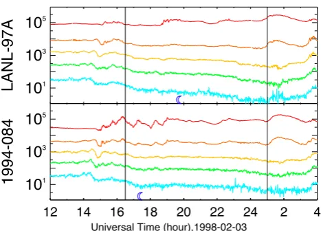
Fig. 2.LANL SOPA Proton data for Event 1. Each color is a different energy channel with red as

the lowest energy and blue as the highest. The blue moon represents when the satellite is at local

midnight. Once again the vertical lines represent the beginning and the ending of the BRI.

23

Fig. 2. LANL SOPA Proton data for Event 1. Each color is a

dif-ferent energy channel with red as the lowest energy and blue as the highest. The blue moon represents when the satellite is at local mid-night. Once again the vertical lines represent the beginning and the ending of the BRI.

final event begins and ends with substorms, it differs from the others because it occurs during a higher level of magne-tospheric activity.

2 Data and methodology

The boundary between open and closed magnetic field lines in the magnetosphere maps approximately to the poleward edge of the aurora (Frank and Craven, 1988; Craven and Frank, 1987). This poleward boundary can be measured us-ing Polar UVI LBHl and IMAGE FUV WIC data. Baker et al. (2000) compared the auroral boundary as measured by Polar UVI LBHl to that of DMSP data. They found that a cutoff brightness of approximately 4.3 photons/cm2/sr (∼130 Rayleighs) compares well to the DMSP open-closed bound-ary. However, when the aurora is active, this intensity cut-off increased and must be subsequently accounted for in the boundary identification. Although this method of finding the open-closed boundary is not exact, it is the temporal changes in this boundary we are interested in. For example, if the im-age boundary shifts or changes then the “true” open-closed boundary is assumed to change by the same amount.

Once the boundaries are found for all the available im-ages during an event, then the area inside the boundary is calculated. This area is the polar cap area (Apc). In order to calculate the total amount of open magnetic flux in the polar cap (Fpc), the total magnetic field is integrated over the po-lar cap area. The International Geomagnetic Reference Field (IGRF) is used to calculate the magnetic field. As stated in the introduction, changes in theFpcindicate an imbalance in the magnetopsheric reconnection rates. Thus, only changes in theFpcremain relevant to this study.

This boundary method shows that, during a substorm ex-pansion phase, theFpcdrops approximately 30% in one hour or less (DeJong et al., 2007). Thus, we adopt the criterion that variations in theFpc must be less than 10% within a 1-h interval during t1-he BRI event. However, small variations, falling well within our error of±5%, occur due to changes in auroral imaging coverage and the boundary threshold (De-Jong and Clauer, 2005). For consistency, all four events are measured using Polar UVI LBHL imaging data. They all also take place during northern winter so dayglow removal was not required.

The indices used in this study (AE, AL, cross polar cap potential (CPCP), andDst) are derived by the assimilative mapping of ionospheric electrodynamics (AMIE) technique (Richmond, 1992), which has been applied to approximately 150 ground-based high-latitude magnetometer records (Ri-dley and Kihn, 2004; Cai et al., 2006). The interplanetary magnetic field (IMF) and solar wind parameters have been propagated to Earth using the Weimer et al. (2002, 2003); Weimer (2004) pseudo-minimum variance technique. The propagation is accurate to approximately 6 min, thus onsets and triggers may not occur at the exact same time.

3 Case studies

3.1 Event 1: Classic BRI (SMC) (3 and 4 February 1998) Figure 1 is a stack plot of data for the BRI that begins at 16:30 UT on 3 February and ends at 01:00 UT on the 4th. The top panel is a MLT-UT plot of the maximum brightness from Polar UVI LBHl images. The center of the plot is mid-night while the top and bottom are noon. Thus, any auroral brightenings associated with substorms should take place to-ward the center of the plot. One such brightening is associ-ated with the substorm that occurs at 15:00 UT on the 3rd. The second panel is the amount of open magnetic flux in the polar cap (Fpc) in GigaWebers (GWb). The next four panels are CPCP (kV), AE (nT), AL (nT), and Dst (nT), all cal-culated from AMIE (Ridley and Kihn, 2004). The Weimer propagated IMFBzis plotted on the bottom panel.

Although this event has previously been studied by Goodrich et al. (2007), it remains a key component of this in-vestigation because it represents a “classic” BRI. This event is described as “classic” since it fits the definition of an SMC set forth by Sergeev and Lennartsson (1988); Sergeev et al. (1996). The IMFBzis steady at approximately−6 nT. AE, AL and Dst all exhibit very little variation. The Fpc re-mains steady at 0.51±0.04 GWb and the aurora is enhanced with very few brightenings and little movement. There are also substorms before and after the BRI, following the more classic definition of an SMC. The first substorm onsets at 15:00 UT and recovers before the BRI starts. Because the Fpc remains steady until the concluding substorm, it is dif-ficult to separate the growth phase of the substorm from the

BRI. Since there is no measurable loading of the tail, the BRI ends with the onset of the expansion phase of the substorm. However, it appears that this substorm was triggered by the IMFBzturning northward at 01:00 UT. Thus, termination of the dayside reconnection causes the tail to unload via a sub-storm.

The two panels on Fig. 2 are plots of Los Alamos National Lab (LANL) synchronous orbit particle analyzer (SOPA) proton data from two different satellites (1995-084 and LANL-97A). There are five different energy channels plot-ted with red as the least energetic and blue as the most. The moon on the plots indicates when the satellite is at local mid-night. There are no large particle injections that would indi-cate a substorms during this event (Walker et al., 1976; Erick-son et al., 1979). There are, however, some small injections at around 18:00, 19:00, and 22:00 UT in the lower energy changes that may be associated with narrow plasma injec-tions. The initiating and concluding substorms have larger particle injections at 15:00 and 01:00 UT, respectively.

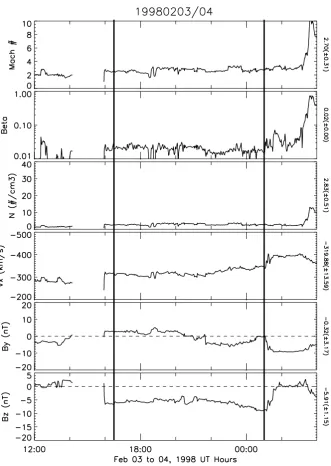
The solar wind/IMF data from the WIND satellite is dis-played in Fig. 3, propagated to Earth using Weimer (2004). The IMFBzduring this BRI/SMC is similar to that of other SMCs as measured by O’Brien et al. (2002) and Tanskanen et al. (2005): negative, steady, and of moderate magnitude (−5.9±1.15 nT). However, it is the very low Alfv´enic Mach number that is intriguing. The Alfv´enic Mach number for the solar wind is very low at 2.7±0.31. It has been noted recently that the magnetospheric interaction with the solar wind may be quite different under low Mach number and lowβ. For example, Lavraud et al. (2007) showed that un-der nominal solar wind conditions, the1P force is dominant in reaccelerating the solar wind in the magnetosheath, while during lowβ cases, theJ×B force is dominant since the magnetic field is dominant. Further, Tanskanen et al. (2005) showed that during low Mach numbers, the magnetosphere has predominant Alfv´en wings, which may strongly influ-ence the solar wind magnetosphere interaction. Saturation of the ionospheric cross polar cap potential occurs under these conditions.

3.2 Event 2: Driven recovery Phase BRI (15 February 1998)

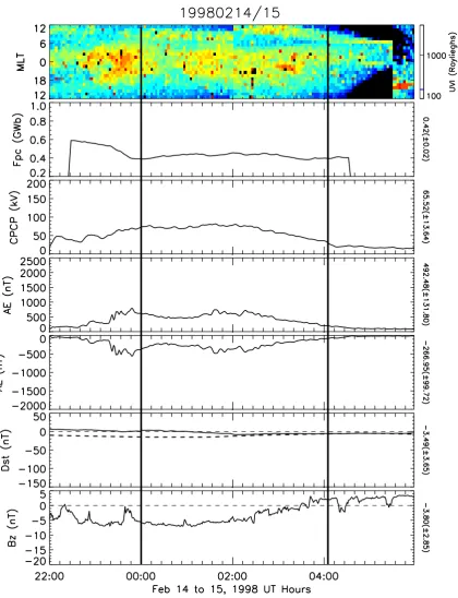
The second BRI occurs on 15 February 1998 and lasts from 00:00 UT to 04:05 UT. While this event is considered a Bal-anced Reconnection Interval, since theFpcremains steady at 0.42±0.02 GWb for over 4 h, the interval would probably be better described as a driven recovery phase. Figure 4 shows a substorm with an expansion phase onset at 22:40 UT, but after the hour long recovery phase theFpc remains steady for 4.25 h and the aurora remains bright. The CPCP, AL, and AE also show a higher level of activity in the auroral zone until 02:16 UT, when they begin to decay to quiet time lev-els (AE 735 to 200 nT, AL−464 to−75 nT, and CPCP 78 to 33 kV). The event ends when AE drops below 200 nT at

04:05 UT. The auroral activity declines as the IMFBzslowly starts to turn northward at about 02:00 UT. The activity re-turns to quiet levels approximately half an hour after the IMF Bzhas turned completely north. It is the extended southward IMFBzand its slow northward turning that allows the mag-netotail to slowly relax back to a quiet state without first un-balancing the reconnection rates. Thus, the recovery phase of the first substorm is still being driven by the IMFBz south-ward until the magnetosphere relaxes.

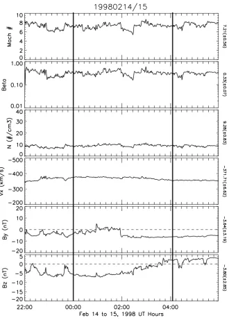
Figure 5 shows the propagated solar wind/IMF data from the ACE satellite. The solar wind during this event appears to be at nominal levels. The Mach number is steady at about 7.2±0.56, while Beta (0.33±0.07) and number den-sity (9.28±0.83 cm−3) are also at “average” levels. The IMF/solar wind data remains fairly steady and Bz appears to be the only major driver during this event.

3.3 Event 3: No substorm to initiate BRI (22 and 23 De-cember 2000)

While the previous BRI started with a substorm and ended when the magnetosphere relaxed back to quiet levels, the BRI on 22–23 December 2000 starts when the magneto-sphere slowly rises to active levels and ends with a substorm. The aurora during this event is stronger and brighter than the last two examined. The BRI starts at 21:42 UT when AE be-comes greater than 200 nT. AE then slowly rises to 946 nT. AL slowly drops (−134 to−541 nT) during this time, indi-cating a slow increase in magnetospheric activity. However, no disruptions that indicate a substorm expansion occur dur-ing this time interval. The top panel of Fig. 6 shows the au-rora slowly becoming more active, but once again, there is no sign of a substorm expansion in the aurora or in other data. At 23:30 UT there is a large northward turning of the IMF Bzthat one would expect to trigger an expansion phase of a substorm. There is a brightening in the aurora at this time close to dawn (18:00 MLT), but there is no response in AL, no westward traveling surge, and poleward expansion of the oval. Thus, it is considered to be a pseudo-breakup (Koski-nen et al., 1993; Kullen and Karlsson, 2004). During the rest of the event, theFpcremains steady at 0.76±0.05 GWb until the substorm at 04:49 UT. Once again it is difficult to sep-arate the BRI and the growth phase of the concluding sub-storm, due to theFpcremaining steady until the onset of the expansion phase. However, during this event the substorm expansion does not appear to be triggered by a northward turing of the IMF Bz. This is similar to the event investi-gated by Yahnin et al. (1994), where there appears to be no trigger for the concluding substorm expansion of the SMC. The reason for the change in reconnection rates is unknown at this time but it is most likely due to an internal process in the magnetosphere.

Fig. 3.

A stack plot of solar wind / IMF parameters from the WIND satellite propagated to the

magnetopause using the Weimer method for Event 1. Solar wind Alfven Mach Number. Solar wind

plasma Beta. Solar wind Dynamic Pressure (nPa). Solar wind Vx (km/s) IMF By (nT) IMF

Bz

(nT).

Once again, the vertical lines represent the beginning and ending of the BRI. The numbers on the

side are the averages and standard deviations for the BRI time frame only.

24

Fig. 3. A stack plot of solar wind/IMF parameters from the WIND satellite propagated to the magnetopause using the Weimer method for

Event 1. Solar wind Alfv´en Mach Number. Solar wind plasma Beta. Solar wind Dynamic Pressure (nPa). Solar wind Vx (km/s) IMF By (nT) IMFBz(nT). Once again, the vertical lines represent the beginning and ending of the BRI. The numbers on the side are the averages and standard deviations for the BRI time frame only.

at 04:00 UT on the 23rd, which implies that the BRI event happens during the main phase of a weak magnetic storm. The difference between these two measurements could indi-cate that there may be a lot of structure in the inner magne-tosphere. When more magnetometers are used, as in theDst from AMIE, they may average out to zero, while, when only 4 magnetometers are used, a more disturbed picture of the inner magnetosphere may arise.

Figure 7 shows the Weimer propagated ACE data for this event. While there is not solar wind data for the entire event, what is shown remains unsteady. At the start of the BRI, the Alfv´enic mach number is 6 and quickly moves up to 9.8. It then drops back down to 2.6 30 min later, rising back to 7 and falling to 2.5 45 min later. At 00:13 UT on the 23rd, it remains weak, at close to 3, until the data ends. The solar wind Beta and number density follow a similar pattern. By

Fig. 4.

A stack plot of the data for the BRI on Feb. 14 and 15, 1998 (Event 2). The set up is the

same as figure 1.

Fig. 4. A stack plot of the data for the BRI on 14 and 15 February 1998 (Event 2). The set up is the same as Fig. 1.

observing just solar wind density or dynamic pressure, one would expect to see a large increase in auroral activity dur-ing this event (Chua et al., 2001; Boudouridis et al., 2003, 2004, 2005), yet there is none. One of the most interesting

Fig. 5.

Propagated ACE data for the BRI on Feb. 14 and 15, 1998 (Event 2). The set up is the same

as figure 3.

26

Fig. 5. Propagated ACE data for the BRI on 14 and 15 February 1998 (Event 2). The set up is the same as Fig. 3.

same time as the spike inBz, the solar windVydrops from 0 to∼−55 km/s and theVzdrops from 0 to∼−80 km/s for ap-proximately 30 min then they both return to zero. This may indicate that the short increase inBzdoes not hit the Earth’s magnetosphere.

3.4 Event 4: Active BRI (17 February 1998)

The last BRI to be investigated occured on 17 February 1998 and shows a slow growth in Fpc after a 5.67 h period of steadiness. Figure 8 shows that there is a substorm expan-sion at 14:15 UT (determined by AL) that precedes the BRI

starting at 15:45 UT when AL becomes steady. Fpc is not used to determine the start of the BRI, because the Polar UVI coverage does not start until 16:00 UT. While there are small perturbations in CPCP, AL, and AE, none of the variations are large enough or last long enough to constitute a sub-storm expansion. AE fluctuates between 585 and 1232 nT with an average of 834 nT, increasing to 1500 nT when the second substorm occurs. AL fluctuates between −277 and −915 nT with an average of−538 nT. While these variations may seem large, compared to the substorms that begin and end the event they are small in size and time scale. Thus,

Fig. 6.

A stack plot of the data for the BRI Dec. 22 and 23, 2000 (Event 3). The set up is the same

as figure 1 and 4

Fig. 6. A stack plot of the data for the BRI 22 and 23 December 2000 (Event 3). The set up is the same as Figs. 1 and 4.

they are not consistent with substorms expansions during this time interval. The event ends at 21:22 when the growth phase of the substorm starts. The two hour long growth phase is not considered part of the BRI, since theFpcincreases by more than 10% per hour during this time.

Fig. 7.

Propagated ACE data for the BRI on Dec. 22 and 23, 2000 (Event 3). The set up is the same

as figures 3 and 5.

28

Fig. 7. Propagated ACE data for the BRI on 22 and 23 December 2000 (Event 3). The set up is the same as Figs. 3 and 5.

merging rate is greater than the nightside reconnection rate (Milan et al., 2007). Milan et al. (2007) investigated a simi-lar nightside reconnection event and suggest that this only oc-curs when theFpcbecomes greater than 0.8 GWb. At the on-set of the substorm at 23:19 UT, theFpcmeasures 0.84 GWb and continues to increase to 0.9 GWb, before it starts to drop at 00:45 UT on the 18th.

This event is moderately active with the CPCP of approx-imately 106 kV and AE at 834 nT. TheDstis dropping from −10 to−80 nT during this event, implying it takes place dur-ing the main phase a geomagnetic storm. The IMFBz is

strong and southward during this event: −8±1.15 nT, such that one might expect to see a periodic sawtooth oscillation (Henderson et al., 2006) instead of balanced reconnection. In order to show that it is not a sawtooth event, the LANL SOPA proton data is shown in Fig. 9. While there are small pertur-bations in the data, there are no signatures of stretching or injections consistent with a substorm or a sawtooth oscilla-tion. The small perturbations appear to be different than the substorms at 14:15 and 23:19 UT where the particle densities drop, as the magnetotail is stretched, and then inject back into the inner magnetosphere during the dipolarizations. Sergeev

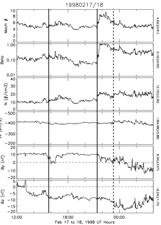
Fig. 8.

A stack plot of the data for the BRI on Feb. 17, 1998 (Event 4). The same set up as figures

1, 4 and 6. The solid black vertical lines represent the beginning and ending of the BRI. The dotted

line is the onset of the substorm at 23:19 UT.

Fig. 8. A stack plot of the data for the BRI on 17 February 1998 (Event 4). The same set up as Figs. 1, 4 and 6. The solid black vertical lines

represent the beginning and ending of the BRI. The dotted line is the onset of the substorm at 23:19 UT.

et al. (2005) also study this event. They show that the small injections seen in the LANL data are associated with bursty bulk flows (BBFs) and auroral streamers. So, there is energy being transferred from the tail into the auroral region but not

10

10

10

1994-084

10

10

10

LANL-97A

12 14 16 18 20 22 24 2 4

Universal Time (hour),1998-02-17

Fig. 9.LANL SOPA Proton data for Event 4. Each color is a different energy channel with red as

the lowest energy and blue as the highest. The blue moon represents when the satellite is at local

midnight and the red star is local noon. Once again, the solid black vertical lines represent the

beginning and the ending of the BRI and the dotted line is the substorm at 23:19 UT.

30

Fig. 9. LANL SOPA Proton data for Event 4. Each color is a

dif-ferent energy channel with red as the lowest energy and blue as the highest. The blue moon represents when the satellite is at local midnight and the red star is local noon. Once again, the solid black vertical lines represent the beginning and the ending of the BRI and the dotted line is the substorm at 23:19 UT.

The solar wind and IMF are steady for the first 5.5 h of the event as shown in Fig. 10. At 21:25 UT, around the same time that theFpcstarts to grow, the density increases from 11 to 20 cm−3_{and remains close to 20 cm}−3_{for the next hour}

and a half. Since both the solar wind velocity and the IMF Bzremain steady during the pressure pulse, it is the increase in density that causes both the Alfv´enic Mach number and the solar wind Beta to increase. This data is in agreement with Ober et al. (2007) who show that an increase in the solar wind density of this type (with other parameters held constant) can cause the open flux in the polar cap to increase. However, Boudouridis et al. (2003, 2004, 2005) have demon-strated that, when a pressure pulse interacts with the magne-tosphere, the auroral will tend to move poleward. Since this is not in agreement with this event, further studies need to be done in order to examine why there is poleward movement in some events and not others.

4 Discussion

The fundamental question that is at issue in the study of SMCs or BRIs is: What allows reconnection rates to bal-ance? Sergeev et al. (1996) suggest that the magnetosphere may need to first unload its tail flux in the form of a sub-storm expansion before the reconnection rates can balance. They propose that SMCs (BRIs) may occur when the plasma sheet is thick, as during the recovery phase, and while theBz driver remains enhanced. Thus, the near-Earth tail develops a growth phase type configuration, while the mid-tail region persists in the expansive state. This magnetospheric configu-ration gives the minimumBzthey measured in the equatorial

magnetic field near 12RE. Although this paper does not ex-plore the tail region during these events, this explanation set forth by Sergeev et al. (1996) does not hold for all the events studied, since Event 3 fails to start will a substorm. It appears that in Event 3 the magnetosphere is already in a state that al-lows the reconnection rates to balance without the need for the recovery and expansion phases discussed by Sergeev et al. (1996). Thus, it seems that preconditioning of the magne-tosphere may play a role in some BRI events.

This investigation shows that there are least three differ-ent situations that can cause the reconnection rates to be-come unbalanced: (1) the dayside reconnection reduces sig-nificantly (Events 1 and 2), (2) the dayside reconnection in-creases without an increase in the nightside rate (increased driving) (Event 4), (3) some internal process causes a sub-storm to occur (Event 3). Events 1 and 2 cease when the dayside reconnection is reduced. In Event 1, the IMF Bz turns northward suddenly, causing a new reconnection point to form, and a substorm ensues. During Event 2, the IMF Bztakes 2 h to turn northward. This allows the reconnection on the nightside to maintain balance, but once the IMFBzis fully northward and reconnection on the dayside is reduced significantly, the event ends. Event 3 appears to end without a trigger in the solar wind/IMF, suggesting a stochastic process causes a new reconnection point to form. Milan et al. (2007) find that 50% of their untriggered tail reconnection events oc-cur when theFpc>0.7 GWb, leading them to conclude that these events happen spontaneously due to stresses in the tail. Event 3 has an averageFpc of 0.76 (±0.05) GWb and con-tains the only untriggered substorm onset. Even though the events of Milan et al. (2007) are not preceded by a BRI, the physics appears to be the same. Finally, Event 4 ends with an increase in dayside reconnection, while the nightside recon-nection presumably stays the same. This causes flux loading in the tail and a growth in theFpc.

Another way to analyze the conclusion of these events is in terms of substorms. Once again 3 different endings for the events were found: (1) substorm growth phase (Event 4), (2) substorm expansion phase (Events 1 and 3), and (3) no sub-storm (Event 2). Events 1 and 3 end abruptly with the appear-ance of a substorm expansion phase in the data. In Event 1 the dayside reconnection rate reduces, causing nightside re-connection to be larger than the dayside and the expansion phases ensues. However, in Event 3 there appears to be no turning off of the dayside reconnection. Event 4 ends when theFpc begins to grow for 2 h preceding the substorm. The growth inFpc is caused by the build up of magnetic flux in the tail that occurs during the growth phase of a substorm.

The solar wind/IMF drivers for all four events are fairly steady. Thus, the notion that SMCs (BRIs) occur when the IMFBz is negative and steady still holds for these events. There are some perturbations in the ACE data for Event 3 that do not appear to impact the BRI. The IMFBzfor all of the events is less than−5 nT. This differs from previous stud-ies that state that steady magnetospheric convection usually

Fig. 10.

Propagated ACE data for the BRI on Feb. 17, 1998 (Event 4). The set up is the same as

figures 3, 5, and 7. Once again, the solid vertical lines represent the beginning and the ending of the

BRI, and the dotted line is the substorm at 23:19 UT.

Fig. 10. Propagated ACE data for the BRI on 17 February 1998 (Event 4). The set up is the same as Figs. 3, 5, and 7. Once again, the solid

vertical lines represent the beginning and the ending of the BRI, and the dotted line is the substorm at 23:19 UT.

occurs when 0 nT>Bz≥−5 nT (Sergeev et al., 1996; O’Brien et al., 2002; Tanskanen et al., 2005). Event 1 has aBzclose to −6 nT and Event 2 starts with aBzof−5 nT before it starts to turn northward. Events 3 and 4 both have a larger magnitude of the IMFBz(−12 and−8 nT, respectively) than expected for this type of event. Another interesting driver to note is the solar wind Beta and Alfv´enic Mach number. With the excep-tion of Event 2, they are all lower than the “average” solar wind beta and Mach number. The solar wind/IMF drivers will be studied in more detail in a future paper that includes

a statistical analysis of the 51 BRI events found using theFpc criteria.

While the drivers during these events are considered rel-atively constant, the magnetospheric data is not as steady. Once again, Events 1 and 2 are the most steady and most closely fall into the category of an SMC. Event 3 has a slow growth in the AL, indicating that the activity in the auroral zone is increasing during this event. There is also an auro-ral brightening or pseudo-breakup during this event. Thus, the magnetosphere is not completely steady, yet the global

reconnection rates are still relatively balanced in a global sense. Event 4 is by far the most active event. There are variations in AL, AE, and CPCP along with an active au-rora. Also,Dst and LANL SOPA proton data indicate that the inner magnetosphere is still dynamic during this event. The variations in the data during Events 3 and 4 are what Sergeev et al. (1996) refer to as “mesoscale transient activa-tions” and can occur during SMC events. However, Event 4 has more activity than any of the events studied by Sergeev et al. (1996). It also has a larger CPCP (106.7±11 kV) than any event they studied, because they only selected events with a CPCP between 60 and 90 kV. Thus, Event 4 is stronger, and therefore, so are the “mesoscale transient activations.” Al-though the last two events are not “steady”, they are classi-fied as BRIs because the global dayside and nightside recon-nection rates balance and they lack signatures of large-scale tail reconfiguration (Sergeev et al., 1996). A further study will investigate statistically the steadiness in the solar wind drivers and auroral zone indices for more BRIs.

The reliance on good, global measurements of the aurora remains one of the main difficulties with utilizing open flux in the polar cap to determine if an event is a BRI or not. This means that events can be missed when satellites are not at a good position to take full auroral images. Also, due to the demise of the IMAGE and POLAR spacecraft, global auroral images are no longer available. With the new ar-ray of ground-based all-sky images in the Canadian sector, it is possible to get nightside imagery of the auroral oval, but this does not allow for an examination of both the day-side and nightday-side flux. Therefore, an improved technique, not reliant upon the global imagery, must be determined. While this is beyond the scope of this study, it is recognized that this is quite important for identifying future BRI events. The 51 events that have been identified can be compared to other techniques used for determining SMCs/BRIs, such as those discussed by O’Brien et al. (2002). Further, other tech-niques must be investigated, such as comparing the dayside and nightside electric fields produced from the AMIE tech-nique or SuperDARN radars, to approximate the reconnec-tion rates. While these techniques will not be perfect, per-haps a combination of methods will allow for proper event selection.

5 Conclusions

This investigation illustrates the diversity of BRIs/SMCs. In order to truly understand the physics behind balanced recon-nection in the magnetosphere, we must broaden our studies of SMCs and redefine them physically as Balanced Recon-nection Intervals. Applying the term “steady” to a system as large and complex as the magnetosphere poses fundamental problems. Convection can remain quasi-steady on a global scale, while small scale perturbations are still occurring. Ul-timately, the only way to achieve this large scale steadiness

is through a balance of dayside and nightside reconnection rates. Thus, the new name of Balanced Reconnection Inter-val (BRI) better describes the physical state of the magneto-sphere than Steady Magnetospheric Convection (SMC).

The measurement of open magnetic flux in the polar cap (Fpc) is a much better indicator of the balance between day-side and nightday-side reconnection rate than auroral indices, such as AL and CPCP. For example, if the reconnection rates stop balancing due to an increase in the dayside reconnection rates, as in Event 4, this can be measured as an increase in the Fpc. However, this change in reconnection rates is difficult to observe in AL or CPCP. This new definition eliminates the need to estimate the concluding time of a BRI in an ad hoc way. Previous studies first determine the onset time of the ex-pansion phase of the concluding substorm and then subtract the average growth phase length to determine the end time of the SMC. This technique may cause BRIs to appear shorter than they actually are. For instance, Events 1 and 3 do not show a growth phase in theFpc, suggesting that the recon-nection rates stay balanced until the onset of the concluding substorm expansion phase. Thus, the new definition of BRI allows for the inclusion of this time period, instead of simply stating that SMCs end with the growth phase. Also, because our method of identifying BRI events is limited by auroral imaging coverage it can be difficult to find a large number of events. Thus, further studies comparing our events to those found using other methods (O’Brien et al., 2002) may help to find a better methodology for identify events than either method is capable off at this moment.

The four BRIs examined in this paper are excellent exam-ples of the diversity of this types of events. While some of the events are more intriguing than others, they all generate challenging questions to be investigated. Since event 1 (3 and 4 February 1998) is a classic BRI/SMC, i poses the most sig-nificant underlying question about these events: “What truly causes reconnection rates to balance?” Event 2 (15 February 1998) is most likely a common type of BRI event and it raises the question: “At what rate canBzturn northward and still allow the magnetosphere to slowly relax into a quiet state?” In other words, is there somedBz/dtthreshold where a con-cluding substorm is or is not triggered? At the conclusion of the third and fourth events (22 and 23 December 2000 and 17 February 1998, respectively) the Solar wind/IMF drivers remain steady, yet one event ends with a substorm growth phase (slow increase in Fpc), and the other ends when the magnetosphere unloads with the onset of a substorm expan-sion phase. Thus, the question is raised: “Is there a point where the reconnection rates just can’t balance anymore and a growth phase or an expansion phase is inevitable?” More events like 2, 3 and 4 need to found and studied in detail and in a statistical manner in order to understand why reconnec-tion rates balance and become unbalanced.

Acknowledgements. The authors would like to thank: Joseph Baker for use of his codes and James Weygand for the propagated solar wind data. Anna DeJong gratefully acknowledges NASA GSRP support through grant NNM04AA05H. Aaron Ridley received sup-port through NSF grant ATM0417839. The authors would also like to acknowledge the NASA grant at Virginia Tech for partial support NNX07AH23G.

Topical Editor I. A. Daglis thanks A. Boudouridis and V. Sergeev for their help in evaluating this paper.

References

Akasofu, S. I.: The development of the auroral substorm, Planet. Space. Sci. 12, 573–578, 1964.

Baker, J. B., Clauer, C. R., Ridley, A. J., Papitashvili, V. O., Brit-tnacher, M. J., and Newell, P. T.: The nightside poleward bound-ary of the auroral oval as seen by DMSP and the Ultraviolet Im-ager, J. Geophys. Res., 105, 21 267–23 280, 2000.

Boudouridis, A., Zesta, E., Lyons, L. R., Anderson, P. C., and Lum-merzheim, D.: Effect of solar wind pressure pulses on the size and strength of the auroral oval, J. Geophys. Res., 108(A4), 8012, doi:10.1029/2002JA009373, 2003.

Boudouridis. A., Zesta, E., Lyons, L. R., Anderson, P. C., and Lummerzheim, D.: Magnetospheric reconnection driven by so-lar wind pressure fronts, Ann. Geophys., 22, 1367–1368, 2004, http://www.ann-geophys.net/22/1367/2004/.

Boudouridis, A., Zesta, E., Lyons, L. R., Anderson, P. C., and Lummerzheim, D.: Enhanced solar wind geoeffective-ness after a sudden increase in dynamic pressure during southward IMF orientation, J. Geophys. Res., 110, A05214, doi:10.1029/2004JA010704, 2005.

Cai, X., Clauer, C. R., and Ridley, A. J.: Statistical analysis of iono-spheric potential patterns for isolated substorms and sawtooth events, Ann. Geophys., 24, 1977–1991, 2006,

http://www.ann-geophys.net/24/1977/2006/.

Chua, D., Parks, G., Brittnacher, M., Peria, W., Germany, G., Spann, J., and Carlson, C.: Energy characteristics of auroral elec-tron precipitation: A comparison of substorms and pressure pulse related auroral activity, J. Geophys. Res., 106(A4), 5945–5956, 2001.

Cowley, S. W. H. and Lockwood, M.: Excitation and decay of solar wind-driven flow in the magnetophere-ionosphere system, Ann. Geophys., 10, 103–115, 1992,

http://www.ann-geophys.net/10/103/1992/.

Craven, J. D. and Frank, L. A.: Latitudinal motions of the aurora during substorms, J. Geophys. Res., 92, 4565–4573, 1987. DeJong, A. D. and Clauer, C. R.: Polar UVI Images to Study Steady

Magnetospheric Convection Events: Initial Results, Geophys. Res. Lett., 32, L24101, doi:10.1029/2005GL024498, 2005. DeJong, A. D., Cai, X., Clauer, C. R., and Spann, J. F.: Aurora

and open magnetic flux during isolated substorms, sawteeth and SMC events, Ann. Geophys., 25, 1865–1876, 2007,

http://www.ann-geophys.net/25/1865/2007/.

Erickson, K. N., Swanson, R. L., Walker, R. J., and Winckler, J. R.: A study of magnetosphere dynamics during auroral electrojet events by observations of energetic electron intensity changes at synchronous orbit, J. Geophys. Res., 84, 931–942, 1979. Frank, L. A. and Craven, J. D.: Imaging results from Dynamics

Explorer 1., Rev. Geophys., 26, 249–283, 1988.

Goodrich, C. C., Pulkkinen, T. I., Lyon, J. G., and Merkin, V. G.: Mangetospheric convection during intermediate driving: Saw-tooth events and steady convection intervals as seen in Lyon-Fedder-Mobarry global MHD simulations, J. Geophys. Res., 112, A08201, doi:10.1029/2006JA012155, 2007.

Henderson, M. G., Reeves, G. D., Skoug, R., Thomsen, M. F., Denton, M. H., Mende, S. B., Immel, T. J., Brandt, P. C., and Singer, H. J.: Mangetospheric and auroral activity during the 18 April 2002 sawtooth event, J. Geophys. Res., 111, A01S90, doi:10.1029/2005JA011111, 2006.

Hughes, J. M. and Bristow, W. A.: SuperDARN observations of the Harang discontinuity during steady magnetospheric convection, J. Geophys. Res., 108(A5), 1185, doi:10.1029/2002JA009681, 2003.

Koshkinen, H. E. J., Lopes, R. E., Pellinen, R. J., Pulkkinen, T. I., Baker, D. N., and Bosinger, T.: Pseudobreakup and Substorm Growth Phase in the Ionosphere and Magnetosphere, J. Geophys. Res., 98(A4), 5801–5813, 1993.

Kullen, A. and Karlsson, T.: On the relation between solar wind, pseudobreakups and substorms, J. Geophys. Res., 109, A12218, doi:10.1029/2004JA010488, 2004.

Lavraud, B., Borovsky, J. E., Ridley, A. J., Pogue, E. W., Thom-sen, M. F., R`eme, H., Fazakerley, A. N., and Lucek, E. A.: Strong bulk plasma acceleration in Earths magnetosheath: A magnetic slingshot effect?, Geophys. Res. Lett., 34, L14102, doi:10.1029/2007GL030024, 2007.

Lyon, J. G., Fedder, J. A., and Mobarry, C. M.: The Lyon-Fedder-Mobarry (LFM) global MHD magnetospheric simu-lation code, J. Atmos. Sol. Terr. Phys., 66, 1333–1350, doi:10.1016/j.jastp.2004.03.020, 2004.

McWilliams, K. A., Pfeifer, J. B., and McPherron, R. L.: Steady magnetospheric convection selection criteria: Implications of global SuperDARN convection measurements, Geophys. Res. Lett., 35, L09102, doi:10:1029/2008GL033671, 2008.

Milan, S. E., Provan, G., and Hubert, B.: Magnetic flux trans-port in the Dungey cycle: A survey of dayside and night-side reconnection rates, J. Geophys. Res., 112, A01209, doi:10.1029/2006JA011642, 2007.

Ober, D. M., Wilson, G. R., Burke, W. J., Maynard, N. C., and Siebert, K. D.: Magnetohydrodynamic simulations of transient transpolar potential responses to solar wind density changes., J. Geophys. Res., 112, A10212, doi:10.1029/2006JA012169, 2007. O’Brien, T. P., Thompson, S. M., and McPherron, R. L.: Steady magnetospheric convection: Statistical signatures in the solar wind and AE, Geophys. Res. Lett., 29, 2143, doi:10:1029/2001GL019113, 2002.

Pytte, T., McPherron, L. R., Hones Jr., E. W., and West Jr., H. I.: Multiple-satellite studies of magnetospheric substorms - Distinc-tion between polar magnetic substorms and convecDistinc-tion-driven negative bays, J. Geophys. Res., 83, 663–679, 1978.

Richmond, A.: Assimilative mapping of ionospheric electrodynam-ics, Adv. Space Res., 12, 59–68, 1992.

Ridley, A. J. and Kihn, E. A.: Polar cap index comparison with AMIE cross polar cap potential, electric field and polar cap area, Geophys. Res. Lett, 31, L07801, doi:10.1029/2003GL019113, 2004.

Sergeev, V. A., Kubyshkina, M. V., Liou, K., Newell, P. T., Parks, G., Nakamura, R., and Mumilkai, T.: Substorms and convection bay compared: auroral and magnetotial dynamics during convec-tion bay, J. Geophys. Res., 106(A9) 18 843–18 856, 2001. Sergeev, V. A., Pellinen, R. J., and Pulkkinen, T. I.: Steady

magne-tospheric convection: a review of recent results, Space Sci. Res., 75, 551–604, 1996.

Sergeev, V. A. and Lannartsson, W.: Plasma sheet at X -20 Re dur-ing steady magnetospheric convection, Planet. Sp. Sci., 36, 353– 370, 1988.

Sergeev, V. A., Yahnin, D. A., Liou, K., Thomsen, M. F., and Reeves, G. D.: Narrow Plasma Streams as a Candidate to Pop-ulate the Inner Magnetosphere, in: The Inner Magnetosphere: Physics and Modeling, edited by: Pulkkinen, T. I., Tsyganenko, N. A., and Friedel, R. H. W., vol. 155 of Washington D.C. Amer-ican Geophysical Union Geophysical Monograph Series, p. 55, 2005.

Siscoe, G. L. and Huang, T. S.: Polar cap inflation and deflation, J. Geophys. Rev., 90(A1), 543–547, 1985.

Tanskanen, E. I., Slavin, J. A., Fairfield, D. H., Sibeck, D. G., Gjer-loev, J., Mukai, T., Ieda, A., and Nagai, T.: Magnetotail response to prolonged southward IMFBzintervals: Loading, unloading, and continuous magnetospheric dissipation, J. Geophys. Res., 110, A03216, doi:10.1029/2004JA010561, 2005.

Walker, R. J., Swanson, R. L., Winckler, J. R., and Erickson, K. N.: Substorm-associated particle boundary motion at synchronous orbit, J. Geophys. Res., 81, 5541–5550, 1976.

Weimer, D. R., Ober, D. M., Maynard, N. C., Burke, W. J., Collier, M. R., McComas, D. J., Ness, N. F., and Smith, C. W.: Variable time delays in the propagation of the inter-planetary magnetic field, J. Geophys. Res., 107(A8), 1210, doi:10.1029/2001JA009102, 2002.

Weimer, D. R., Ober, D. M., Maynard, N. C., Burke, W. J., Collier, M. R., McComas, D. J., Ness, N. F., Smith, C. W., and Water-mann, J.: Predicting interplanetary magnetic field (IMF) propa-gation delays times using minimum variance technique, J. Geo-phys. Res., 108(A1), 1026, doi:10.1029/2002JA009405, 2003. Weimer, D. R.: Correction to “Predicting interplanetary

mag-netic field (IMF) propagation delays times using minimum variance technique”, J. Geophys. Res., 109(A12), A12104, doi:10.1029/2004JA010491, 2004.

Yahnin, A., Malkov, M. V., Sergeev, V. A., Pellinen, R. J., Aulamo, O., Vennerstrom, S., Friis-Christensen, E., Lassen, K., Danielsen, C., Craven, J. D., Deehr, C., and Frank, L. A.: Fea-tures of steady magnetospheric convection, J. Geophys. Res., 99(A3), 4039–4051, 1994.