Biogeosciences, 10, 5817–5830, 2013 www.biogeosciences.net/10/5817/2013/ doi:10.5194/bg-10-5817-2013
© Author(s) 2013. CC Attribution 3.0 License.
EGU Journal Logos (RGB)
Advances in
Geosciences
Open Access
Natural Hazards
and Earth System
Sciences
Open AccessAnnales
Geophysicae
Open AccessNonlinear Processes
in Geophysics
Open AccessAtmospheric
Chemistry
and Physics
Open AccessAtmospheric
Chemistry
and Physics
Open Access DiscussionsAtmospheric
Measurement
Techniques
Open AccessAtmospheric
Measurement
Techniques
Open Access DiscussionsBiogeosciences
Open Access Open Access
Biogeosciences
Discussions
Climate
of the Past
Open Access Open Access
Climate
of the Past
Discussions
Earth System
Dynamics
Open Access Open Access
Earth System
Dynamics
DiscussionsGeoscientific
Instrumentation
Methods and
Data Systems
Open Access
Geoscientific
Instrumentation
Methods and
Data Systems
Open Access DiscussionsGeoscientific
Model Development
Open Access Open Access
Geoscientific
Model Development
DiscussionsHydrology and
Earth System
Sciences
Open AccessHydrology and
Earth System
Sciences
Open Access DiscussionsOcean Science
Open Access Open Access
Ocean Science
Discussions
Solid Earth
Open Access Open Access
Solid Earth
Discussions
The Cryosphere
Open Access Open Access
The Cryosphere
DiscussionsNatural Hazards
and Earth System
Sciences
Open Access
Discussions
Data-based modelling and environmental sensitivity of vegetation in
China
H. Wang1, I. C. Prentice1, 2, and J. Ni3
1Department of Biological Sciences, Macquarie University, Sydney, Australia
2AXA Chair of Biosphere and Climate Impacts, Department of Life Sciences and Grantham Institute for Climate Change,
Imperial College, London, UK
3State Key Laboratory of Environmental Geochemistry, Institute of Geochemistry, Chinese Academy of Science, Guiyang,
China
Correspondence to: H. Wang ([email protected])
Received: 27 October 2012 – Published in Biogeosciences Discuss.: 3 January 2013 Revised: 25 July 2013 – Accepted: 26 July 2013 – Published: 4 September 2013
Abstract. A process-oriented niche specification (PONS)
model was constructed to quantify climatic controls on the distribution of ecosystems, based on the vegetation map of China. PONS uses general hypotheses about bioclimatic con-trols to provide a “bridge” between statistical niche models and more complex process-based models. Canonical corre-spondence analysis provided an overview of relationships be-tween the abundances of 55 plant communities in 0.1◦grid cells and associated mean values of 20 predictor variables. Of these, GDD0 (accumulated degree days above 0◦C),
Cramer–Prenticeα(an estimate of the ratio of actual to equi-librium evapotranspiration) and mGDD5(mean temperature
during the period above 5◦C) showed the greatest predictive power. These three variables were used to develop general-ized linear models for the probability of occurrence of 16 vegetation classes, aggregated from the original 55 types by k-means clustering according to bioclimatic similarity. Each class was hypothesized to possess a unimodal relationship to each bioclimate variable, independently of the other vari-ables. A simple calibration was used to generate vegetation maps from the predicted probabilities of the classes. Mod-elled and observed vegetation maps showed good to excellent agreement (κ=0.745). A sensitivity study examined mod-elled responses of vegetation distribution to spatially uniform changes in temperature, precipitation and [CO2], the latter
included via an offset toα(based on an independent, data-based light use efficiency model for forest net primary pro-duction). Warming shifted the boundaries of most vegetation classes northward and westward while temperate steppe and
desert replaced alpine tundra and steppe in the southeast of the Tibetan Plateau. Increased precipitation expanded mesic vegetation at the expense of xeric vegetation. The effect of [CO2] doubling was roughly equivalent to increasing
precip-itation by ∼30 %, favouring woody vegetation types, par-ticularly in northern China. Agricultural zones in northern China responded most strongly to warming, but also bene-fited from increases in precipitation and [CO2]. These results
broadly conform to previously published findings made with the process-based model BIOME4, but they add regional de-tail and realism and extend the earlier results to include crop-ping systems. They provide a potential basis for a broad-scale assessment of global change impacts on natural and managed ecosystems.
1 Introduction
achieved in equilibrium with climate – is that it allows di-rections of change in response to environmental changes to be characterized irrespective of lags in the establishment of new vegetation types, or in the responses of agricultural sys-tems to changed conditions. Dynamic modelling of natural changes in vegetation is well established, yet there are still major differences among models (e.g. Sitch et al., 2008), and dynamic modelling of land use change is at an early stage (e.g. Rounsevell et al., 2012). The usefulness of dynamic models depends strongly on their ability to correctly predict directions of change, i.e. the potential distribution to which the dynamic processes are tending. With huge advances in the availability of relevant observations to constrain models, and in the size of problems that can now be tackled using sta-tistical methods, there is considerable scope to develop rela-tively simple models, which are informed by process under-standing but also firmly based on observations (see e.g. Smith et al., 2013).
Anthropogenic climate change is beginning to shift the po-tential and actual spatial patterns of ecosystems and species. This much is clear from thousands of observations world-wide of both expansions and contractions in species’ ob-served ranges and phenologies (Rosenzweig et al., 2007). Climate change is also creating conditions whereby certain types of agriculture are increasingly marginal in some re-gions (e.g. wheat growing in southwestern Australia (How-den et al., 1999) and paddy rice planting in northern China (Li and Wang, 2010)). In other regions, new modes of agri-culture may be starting to become viable. These changes so far have been subtle because climate change has been rela-tively small in a global context, especially when compared with natural interannual variability. But some degree of con-tinuing climate change is unavoidable, and its effects are ex-pected to become increasingly prominent during the coming decades (Prentice et al., 2012). It is useful to foresee at least the direction of such effects, even if their eventual magni-tudes remain largely unpredictable.
The concentration of carbon dioxide ([CO2]) itself has
been recognized as a potentially important non-climatic fac-tor that is already shifting vegetation patterns through its effect on the competition between woody and herbaceous plants through an increase in the water use efficiency of C3
plants, in addition to its effects on climate through the green-house effect. This physiological effect of CO2is a prominent
candidate to explain “woody thickening”, the tendency for trees and shrubs to increase in abundance at the expense of grasses, as has been observed in savannas worldwide (Pren-tice et al., 2011). CO2 concentration also has an enhancing
effect on the growth and yield of C3crops, although the rise
in [CO2] to date is thought to have been only a relatively
minor factor in increasing crop yields (compared with crop breeding and other technological advances; Easterling et al., 2007) and the positive effects may increasingly be offset by negative effects of warming, especially in hot climates (Antle et al., 2002).
So-called niche models or species distribution models – empirical models fitted to species presence or abundance data as a function of climate variables using statistical methods – have been widely and successfully used to describe the relationships between species distributions and climate (Pe-terson, 2001), and more controversially to project responses to future environmental changes (Warren, 2012; Pearson and Dawson, 2003). One key limitation of niche models as usu-ally implemented is that their responses are strongly depen-dent on the choice of environmental predictors (Peterson, 2001). The selection of predictors is usually somewhat ar-bitrary. Such models often rely on ordinary meteorological summary variables (such as mean annual precipitation) that are only indirectly related to the environment “experienced” by the biota. Alternatively, in the BIOCLIM strand of mod-elling, an attempt is made to represent bioclimate, but this is done through the use of a set of ad hoc combinations of vari-ables such as “annual temperature range” and “precipitation of the warmest quarter” (Beaumont et al., 2005). The prob-lem of equifinality in the choice of predictors is not entirely avoidable, because correlations among different aspects of climate mean that the “correct” predictors cannot be chosen unambiguously on the basis of empirical correspondences alone. It is therefore valuable to make use of basic process understanding of the mechanisms controlling species’ via-bility (Harrison et al., 2010) to derive composite bioclimatic variables expressing different aspects of the environment. Furthermore, it is reasonable to assume that different types of environmental requirements (for example, for warmth and moisture availability) act independently. This assumption al-lows a considerable simplification of the modelling process (e.g. Sykes et al., 1996). A further limitation of niche mod-els as usually applied is that they do not include the modi-fying effects of changes in CO2concentration, even though
these are potentially very important (Keenan et al., 2011) and are absolutely required in order to account for the nature of observed, major vegetation changes over glacial–interglacial cycles (Harrison and Prentice, 2003; Prentice and Harrison, 2009; Prentice et al., 2011; Bragg et al., 2013).
study by Gallego-Sala and Prentice (2013), who modelled the world distribution of the blanket bog biome and its re-sponse to climate change based on three independent biocli-matic limits. Here we apply a PONS approach to model the natural and managed vegetation of China, and we demon-strate a novel method by which CO2 effects can be
incor-porated into a niche model. The approach is innovative in combining a well-established technique in statistical niche modelling (multiple logistic regression, which is closely re-lated to the popular maximum entropy method; Phillips et al., 2006) with algorithms used to estimate bioclimatic variables for dynamic vegetation and biogeochemistry modelling, and a process-based method to take account of CO2
concentra-tion effects. By fitting models with linear and quadratic (but not interaction) terms for each predictor, our modelling ap-proach is consistent with Boucher-Lalonde et al. (2012), who showed that the probabilities of occurrence of tree species in North America could be predicted with high efficiency from independent Gaussian functions of climate variables.
2 Methods
2.1 Study area
China, with the third largest land area of any country, con-tains almost the entire range of world vegetation types from rainforest to desert and from tropical to alpine vegetation (Fig. 1). Furthermore, due to its large population and rapid economic development, China is a key region where it is important to identify potential risks and opportunities both for the productivity and carbon storage of natural ecosystems and for the production of food in agricultural systems.
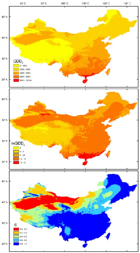
Temperature variables generally decrease from south to north in China. Elevation changes interrupt the latitudinal trend, notably the extremely high and cold area of the Tibetan Plateau, and some low-lying and hot areas in the northwest. Moisture supply from the Pacific and Indian oceans gradu-ally declines from the south towards the north and the in-terior (Fig. 2). The natural vegetation patterns reflect these temperature and moisture gradients (Fig. 1). The diversity of agricultural systems is also closely related to climate. For ex-ample, the Loess Plateau (see Supplement Figure for the dis-tribution of geographical regions in China) and some valleys in the interior of western China experience a moisture regime similar to that of northeastern China, but are much warmer in winter, allowing orchards to grow as well as annual crops (Fig. 1). However in north China especially, irrigation is ex-tensive, and it extends the climatic range of temperate crops towards drier regions provided there is a local supply of wa-ter for irrigation.
2.2 Data
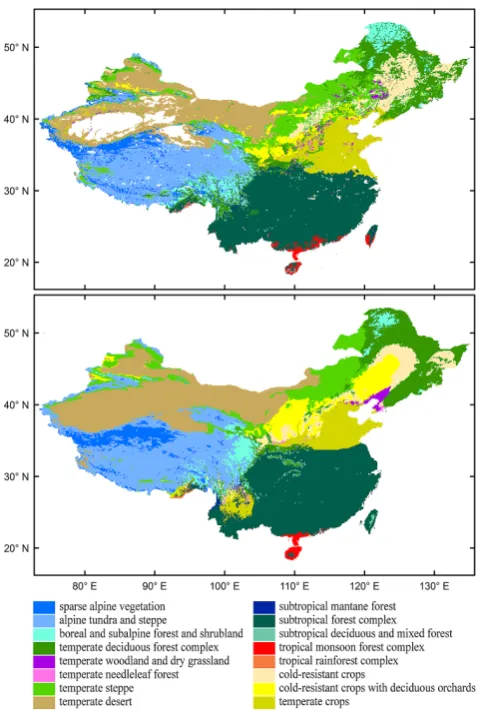
The baseline climatology data were derived from records of mean monthly temperature, precipitation and
percent-Fig. 1. The observed (upper panel) and predicted (lower panel) veg-etation distribution in China. The plant communities from the Vege-tation Atlas of China at a scale of 1:1 million (Hou, 2001) were ag-gregated into 16 vegetation classes based on their bioclimatic con-text.
age of possible sunshine hours at 1814 meteorological sta-tions (740 stasta-tions have observasta-tions from 1971 to 2000, the rest from 1981 to 1990; China Meteorological Admin-istration, unpublished data), interpolated to a 0.01◦grid us-ing a three-dimensional thin-plate spline (ANUSPLIN ver-sion 4.36; Hancock and Hutchinson, 2006). We selected the following 20 predictor variables, calculated as in Prentice et al. (1993) and Gallego-Sala et al. (2011), for an initial ex-ploratory multivariate analysis:
– mean temperature of the coldest (MTCO, ◦C) and warmest (MTWA,◦C) months
– mean annual temperature (MAT,◦C) and precipitation (MAP, mm)
– accumulated (GDD0, ◦C; GDD5, ◦C) and mean
[image:3.595.306.546.64.420.2]Fig. 2. The distribution pattern of the three bioclimatic predictors used to construct models for each vegetation class: annual accumu-lated temperature above 0◦C (GDD0), mean temperature of the pe-riod above 5◦C (mGDD5), and the Cramer–Prentice index of
plant-available moisture (α).
growing season, taking 0◦C and 5◦C respectively as the base temperature
– total (PAR0, mol photon m−2; PAR5, mol photon
m−2) and mean (mPAR0, mol photon m−2; mPAR5,
mol photon m−2) photosynthetically active radiation during the growing season, defined as the period above 0◦C and 5◦C respectively
– annual equilibrium evapotranspiration (PET, mm a−1), moisture index (MI, dimensionless) defined as the ra-tio of MAP to PET, and the Cramer–Prentice
plant-available moisture index (α, dimensionless) (Prentice et al., 1993) calculated as the ratio of annual actual to equi-librium evapotranspiration. Actual evapotranspiration is calculated by a soil moisture-accounting scheme as the daily integral of the lesser of a demand term (PET) and a supply term which is 1 mm h−1times current soil moisture (as a fraction of available water-holding capac-ity). The calculation is based on monthly climatological data, interpolated to a daily time step, and repeated over a sequence of years until the annual cycle of soil mois-ture converges.
– Three additional dimensionless variables were selected
to reflect the seasonal concentration (seasonality) and the sine (Timingsin)and cosine (Timingcos)of the
tim-ing of maximum precipitation (Harrison et al., 2003). Seasonality ranges from 0 (uniform through the year) to 1 (all in one month). Timing ranges from 0 (for precipi-tation centred on January) throughπ/2 (April),π(July), 3π/2 (October) and back to 2π(January). The cosine of timing thus ranges from−1 (summer dominant) to +1 (winter dominant) while the sine ranges from−1 (au-tumn dominant) to +1 (spring dominant).
– We also included two variables (NPPLUEand NPPWUE,
in g C m−2a−1), which are estimates of annual potential net primary production (NPP) based on the light- and water-use efficiency models (Wang et al., 2012), fitted independently to an extensive forest production data set (Luo, 1996).
Table 1. Allocation of observed plant communities from the Vegetation Atlas of China at a scale of 1:1 million (Hou, 2001) to vegetation classes, based onk-means clustering with modifications as described in the text.
Vegetation classes Plant communities
Sparse alpine vegetation 1) Alpine sparse vegetation;
2) alpine cushion dwarf semi-shrubby desert; 3) alpine cushion vegetation
Alpine tundra and steppe 4) Alpine tundra;
5) alpine grass, carex steppe; 6) alpine Kobresia spp., forb meadow Boreal and subalpine forest
and shrubland
7) Cold-temperate and temperate mountains needleleaf forest; 8) subalpine broadleaf deciduous scrub;
9) subalpine broadleaf evergreen sclerophyllous scrub; 10) subalpine broadleaf needleleaf evergreen scrub; 11) alpine swamp
Temperate deciduous forest complex
12) Temperate mixed needleleaf and broadleaf deciduous forest; 13) temperate broadleaf deciduous forest;
14) temperate grass-forb meadow steppe; 15) temperate grass and forb meadow;
16) temperate grass, carex and forb swamp meadow; 17) subtropical and tropical mountains needleleaf forest; 18) cold-temperate and temperate swamp;
19) one crop annually short growing period cold-resistant crops Temperate woodland and dry
grassland
20) Temperate microphyllous deciduous woodland; 21) temperate grass-forb community
Temperate needleleaf forest 22) Temperate needleleaf forest Temperate steppe 23) Temperate needlegrass arid steppe;
24) temperate dwarf needlegrass, dwarf semi-shrubby desert steppe; 25) temperate broadleaf deciduous scrub
Temperate desert 26) Temperate dwarf semi-arboreous desert; 27) temperate shrubby desert;
28) temperate shrubby steppe desert;
29) temperate semi-shrubby and dwarf semi-shrubby desert; 30) temperate succulent holophytic dwarf semi-shrubby desert; 31) temperate annual graminoid desert;
32) temperate grass and forb holophytic meadow
Subtropical montane forest 33) Subtropical mountains mixed needleleaf, broadleaf evergreen and deciduous forest; 34) subtropical broadleaf evergreen sclerophyllous forest
Subtropical forest complex 35) Subtropical needleleaf forest; 36) subtropical broadleaf evergreen forest; 37) subtropical monsoon broadleaf evergreen forest;
38) subtropical and tropical bamboo forest and bamboo scrub; 39) subtropical and tropical broadleaf evergreen and deciduous scrub; 40) subtropical and tropical evergreen xeromorphic succulent thorny scrub; 41) subtropical and tropical grass-forb community;
42) subtropical and tropical swamp;
43) two crops containing upland and irrigation annually, evergreen and deciduous orchards, economic forest; 44) two crops or three crops containing upland and irrigation rotate crops annually (with double-cropping rice), evergreen orchards and subtropical economic forest
Subtropical deciduous and mixed forest
45) Subtropical broadleaf deciduous forest;
46) subtropical mixed broadleaf evergreen and deciduous forest Tropical monsoon forest
complex
47) Tropical monsoon rainforest; 48) tropical mangrove;
49) three crops annually, tropical evergreen orchards and economic forest Tropical rainforest complex 50) Tropical rainforest;
51) tropical needleleaf forest;
52) tropical coral limestone broadleaf evergreen succulent scrub and dwarf forest Cold-resistant crops 53) One crop annually and cold-resistant economic crops
Cold-resistant crops with deciduous orchards
54) One crop annually, cold-resistant economic and deciduous orchards
cold-resistant economic and deciduous orchards”; and “three crops two years and two crops annually non-irrigation, de-ciduous orchards”) in north China were separated from the clusters to which they had been assigned, as the climatic moisture range occupied by these types (due to irrigation) exceeds that of otherwise bioclimatically similar natural veg-etation types. Except for “one crop annually short growing period cold-resistant crops”, with a similar climatic space to the temperate deciduous complex, all the other cultivation systems are typical of south China and share the same bio-climatic space as the natural plant communities there. These cultivation types were therefore kept within their machine-identified vegetation classes (tropical monsoon forest com-plex or subtropical forest comcom-plex).
Accurate fractional areas of each class were extracted in ArcGIS from the digitized vegetation map at 0.1◦grid reso-lution. The bioclimatic data were up-scaled from the original 0.01◦grid to the same 0.1◦grid by simple averaging.
2.3 Data analysis
Canonical correspondence analysis (CCA; Ter Braak and Prentice, 1998) was carried out based on 94 510 records for the 16 vegetation classes and (as predictors) the 20 predictor variables, for an initial exploration of the relationships be-tween climate and vegetation. Non-vegetation grid cells (the white area in Fig. 1), such as glaciers, bare ground, and lakes, were excluded. The Akaike information criterion was used to select the three most important among the bioclimatic vari-ables for further analysis.
Generalized linear modelling (GLM) was applied to each vegetation class separately, using the logit link function and assuming a binomial distribution of the class frequencies. This analysis is equivalent to multiple logistic regression. The input data were the frequency of the class, and values of the three selected bioclimatic predictors, at the grid cells. In each case, we fitted an initial model including linear and quadratic terms for each bioclimatic variable. In some cases, one or more terms were excluded after this initial step, and a new model fitted. Three criteria determined the exclusion of particular terms:
(a) Terms whose inclusion led to unrealistic partial relation-ships. This situation was sometimes encountered due to high correlation between mGDD5 and GDD0 in both
the coldest and the warmest range of climates. The in-clusion of both predictors resulted in sparse alpine veg-etation, alpine tundra and steppe apparently responding positively to GDD0, although they are more abundant
in colder climates. We therefore rejected GDD0 as a
predictor in these cases. Conversely, mGDD5 was
re-jected as a predictor for tropical forests, since the GLM-predicted probability curve against mGDD5peaked at a
very low value compared with the real distribution of tropical forests.
(b) In a few cases, inclusion of quadratic terms resulted in a U-shaped (rather than Gaussian) fitted distribu-tion to a particular variable. This result led to the re-jection of mGDD5as a predictor for temperate desert.
Sparse alpine vegetation, boreal and subalpine forest and shrubland also showed initial fitted U-shaped re-sponses toα. In these cases just the quadratic term was rejected, leading to a realistic (sigmoid) response toα. (c) Terms for which the coefficients were not significant at
P <0.05 were rejected. These cases were few because of the very large sample size.
With the estimated regression coefficients and intercept from the final fitted GLM, a predictive model is obtained for each vegetation class. This can be written in a simple generic form:
ln Pi 1−Pi =a
i
1+b
i
1×α+b
i
2×α 2+ci
1×mGDD5 (1)
+ci2×mGDD2 5+d
i
1×GDD0×10
−3
+d2i×GDD2 0×10
−6,
where Pi is the GLM-predicted probability for vegetation classi anda,b,c,d are parameters specific for each veg-etation class and for each of three predictor variables: α, mGDD5and GDD0. The parameter values for the finally
ac-cepted models are listed in Table 2.
A simple linear calibration was used to relate fitted prob-abilities optimally to observed frequencies, as follows. For each vegetation type, we performed the following ordinary linear regression of the GLM-predicted class probabilities (Pi)on the observed class frequencies (fi0) withm1andm2
as the regression parameters.
Pi =mi1+mi2×fi0 (2)
This regression relationship was then inverted as Eq. (3) to obtain the weighting factors (l1i andl2i, Table 3) to be applied to the GLM-predicted probabilities (Pi)and the calibrated predicted probabilities (fi∗), which were finally used in gen-erating the predicted vegetation distribution map (Fig. 1):
fi∗=li1+l2i×Pi. (3)
Negative values arising from this step were set to zero. The predicted vegetation class at each grid cell is then the one with highest predicted probability after weighting, i.e. the one with highestfi∗. We also predicted the potential natu-ral vegetation class at each grid cell by applying the same criterion but excluding agricultural classes from considera-tion.
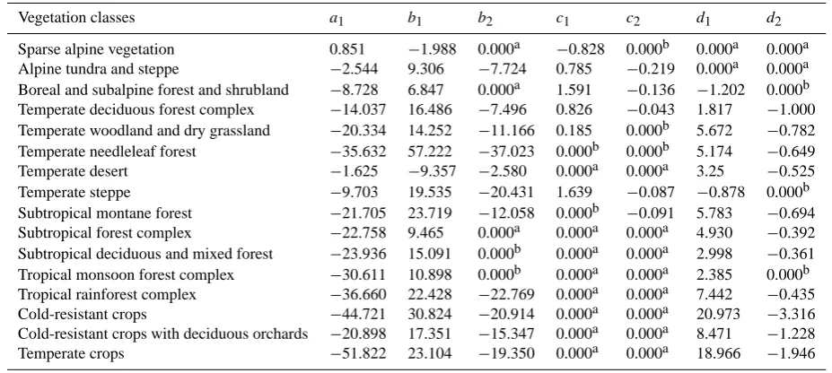
Table 2. Parameters used in Eq. (1) for each vegetation class. All parameters are statistically significant atp <0.001 exceptb1andb2for
subtropical montane forest significant atp <0.05.
Vegetation classes a1 b1 b2 c1 c2 d1 d2
Sparse alpine vegetation 0.851 −1.988 0.000a −0.828 0.000b 0.000a 0.000a Alpine tundra and steppe −2.544 9.306 −7.724 0.785 −0.219 0.000a 0.000a Boreal and subalpine forest and shrubland −8.728 6.847 0.000a 1.591 −0.136 −1.202 0.000b Temperate deciduous forest complex −14.037 16.486 −7.496 0.826 −0.043 1.817 −1.000 Temperate woodland and dry grassland −20.334 14.252 −11.166 0.185 0.000b 5.672 −0.782 Temperate needleleaf forest −35.632 57.222 −37.023 0.000b 0.000b 5.174 −0.649
Temperate desert −1.625 −9.357 −2.580 0.000a 0.000a 3.25 −0.525
Temperate steppe −9.703 19.535 −20.431 1.639 −0.087 −0.878 0.000b
Subtropical montane forest −21.705 23.719 −12.058 0.000b −0.091 5.783 −0.694 Subtropical forest complex −22.758 9.465 0.000a 0.000a 0.000a 4.930 −0.392 Subtropical deciduous and mixed forest −23.936 15.091 0.000b 0.000a 0.000a 2.998 −0.361 Tropical monsoon forest complex −30.611 10.898 0.000b 0.000a 0.000a 2.385 0.000b Tropical rainforest complex −36.660 22.428 −22.769 0.000a 0.000a 7.442 −0.435 Cold-resistant crops −44.721 30.824 −20.914 0.000a 0.000a 20.973 −3.316 Cold-resistant crops with deciduous orchards −20.898 17.351 −15.347 0.000a 0.000a 8.471 −1.228
Temperate crops −51.822 23.104 −19.350 0.000a 0.000a 18.966 −1.946
aandbdistinguish predictor terms excluded due to lack of realism in the fitted model and statistical significance, respectively. See text for further explanation of these criteria.
rainforest complex must exceed 12◦C. The calibrated pre-dicted probabilityfi∗ for this vegetation class was reset to zero whenever this constraint was not met. The constraint has no effect on the predicted present distributions but was intro-duced in order to eliminate the unrealistic prediction of trop-ical rainforest in dry inland areas under some climate change scenarios. The constraint is consistent with the known re-quirement of tropical trees for warm winters.
2.4 Assessing goodness of fit
The kappa statistic (Cohen, 1960; Prentice et al., 1992) was used to quantify the similarity between the predicted and ob-served vegetation maps. Kappa is a suitable measure to com-pare two maps where the variable mapped is a multi-class, qualitative variable. Kappa ranges from zero to one. One means perfect agreement; zero means agreement that is no better than would be expected by chance, i.e. by random as-signment of classes to grid cells.
2.5 Inclusion of a CO2effect
[CO2] does not vary significantly in space, and cannot
there-fore be used as a predictor in the development of empirically based models for vegetation and productivity. As a measure of the effect of increased [CO2] on vegetation distribution,
we estimated the increase inαthat would produce the same gain in NPP, according to a process-oriented light-use effi-ciency (LUE) model that has been fitted independently to an extensive forest production data set (Wang et al., 2012). This approach is based on the assumption that the major effect of elevated [CO2] on vegetation distribution is to enhance
Table 3. Parameters used in Eq. (3) for each vegetation class.
Vegetation l1 l2
Sparse alpine vegetation −0.059 2.257 Alpine tundra and steppe −0.071 1.524 Boreal and subalpine forest and shrubland −0.055 2.123 Temperate deciduous forest complex −0.094 1.885 Temperate woodland and dry grassland −0.123 13.06 Temperate needleleaf forest −0.064 16.426
Temperate desert −0.049 1.347
Temperate steppe −0.116 2.223
Subtropical montane forest −0.011 6.574 Subtropical forest complex −0.058 1.285 Subtropical deciduous and mixed forest −0.07 13.75 Tropical monsoon forest complex −0.009 2.007 Tropical rainforest complex −0.004 2.784
Cold-resistant crops −0.089 2.844
Cold-resistant crops with deciduous orchards −0.191 7.970
Temperate crops −0.056 1.890
water use efficiency (Keenan et al., 2013), which is equiva-lent to increasing water availability. To estimate this equiv-alence, we fitted a multiple regression of the logarithm of forest NPP (data as in Wang et al., 2012) againstα, mGDD5
and GDD0. The log transformation implies for the
underly-ing model that the effects of climate variables on NPP are multiplicative. Then the contribution ofα(dimensionless) to NPP (g C m−2a−1)can be expressed as
ln NPP=a×α+b. (4)
[image:7.595.310.544.361.548.2]mGDD5and GDD0together, which will then be eliminated
in deriving “effective”αat elevated [CO2]. Figure 3 shows
the relationship between ln NPP andα.
The LUE model of Wang et al. (2012) is used to estimate the effect of elevated [CO2] on NPP, indicated by the ratio
(x)of NPP (g C m−2a−1)at elevated (NPP0) and reference (NPP0)[CO2]. According to this model, the ratio is
depen-dent on the leaf-internal [CO2] at reference [CO2] (ci, ppm), the leaf-internal [CO2] at elevated [CO2] (ci0, ppm) and the CO2 compensation point (0, ppm), which is
temperature-dependent (Bernacchi et al., 2003):
x= NPP 0
NPP0
=(c 0
i−0)×(ci+2×0)
(c0i+2×0)×(ci−0). (5) The “effective” value ofαat elevated [CO2] (α0) is then given
by
α0=1
a ×lnx+α. (6)
2.6 Sensitivity analysis
Sensitivity analysis was carried out to investigate the re-sponse of the predicted vegetation pattern to the separate and combined effects of a large increase in temperature, in-crease or dein-crease in precipitation and inin-crease of [CO2],
applied uniformly across the region. For comparability with previously published results using the global BIOME4 model (Wang et al., 2011), we applied the same environmental changes as in that paper. Thus the mean temperature of each month was increased by 5 K, the mean precipitation of each month was increased or decreased by 30 %, and [CO2] was
doubled from a reference value of 376 to 732 ppm. These changes were applied separately and in combination.
3 Results
3.1 Data analysis
The triangular pattern illustrated by the CCA biplot summa-rizes the climate–vegetation relationship in China (Fig. 4a). The vertex of the triangle to the right of the biplot rep-resents the extreme of high temperature, rainfall and pro-ductivity in south China. The other two vertices repre-sent the dry and cold extremes, respectively, exemplified by the interior deserts (upper left) and the high eleva-tions of the Tibetan Plateau (lower left). Energy-related variables (mGDD5, MTWA, mGDD0, PAR5, PAR0, PET,
GDD0, GDD5, MAT) and primary production (NPPLUEand
NPPWUE)tend to align together, pointing towards the
[image:8.595.311.547.60.226.2]high-productivity vertex. Moisture-related variables (MI,α, MAP) point in a direction opposite to the dry vertex. The shape of this diagram indicates the fundamental trade-off between high annual productivity (associated with climates that are both warm and wet) and tolerance of dry or cold conditions,
Fig. 3. Partial residual plot (Breheny and Burchett, 2013) of ob-served NPP (natural log scale) against the Cramer–Prenticeαindex of plant-available moisture. The partial regression line with confi-dence band as shown was based on a multiple regression of ln NPP againstα, GDD0and mGDD5.
i.e. both dry and cold conditions are incompatible with high productivity. The two precipitation timing variables point to-wards the high-productivity vertex, consistent with the fact that both cold and dry vegetation classes are associated with strong summer or autumn rainfall maxima. Precipitation sea-sonal concentration points away from the high-productivity vertex, consistent with the negative effect of a prolonged dry season on total annual productivity. As the length of the thermal growing season declines towards cold climates, both mPAR0 and mPAR5 increase (because the growing season
is increasingly restricted to the summer, when solar radia-tion is at a maximum). Therefore, the direcradia-tion of mPAR0
is almost opposite to MTCO. That the direction of mPAR5
is somewhat different to that of mPAR0 is consistent with
the fact that the cold-resistant vegetation types tend to have cloudy conditions when temperatures exceed 5◦C, whereas xeric vegetation types tend to have more sunny conditions.
The three variables GDD0, mGDD5 and α collectively
can predict almost exactly the same pattern as in Fig. 4a (see Fig. 4b). GDD0 expresses the direction towards
high-productivity vegetation;αexpresses the direction away from dry conditions; mGDD5expresses the direction towards cold
conditions.
3.2 Model testing
Fig. 4. Biplot of plant communities and environmental variables with all sample sites (grey dots) from canonical correspondence analysis using (a) 20 predictor variables, and (b) a subset of 3 pre-dictor variables selected using the Akaike information criterion. See text for the abbreviations of environmental variables, and Table 1 for the code numbers of plant communities. Vegetation classes are distinguished with colours as in the legend of Fig. 1.
as “substantial” agreement according to the criteria of Cohen (1960) and “good” (but very close to “excellent”) agreement according to Monserud (1990).
The predicted vegetation map successfully captures the distributions and boundaries of most vegetation types in China. The distribution of the subtropical forest complex (the most widely distributed forest class in China) is slightly over-estimated, extending into areas occupied by tropical rainfor-est along the south coast and northward into the temperate crop region in the north. The tropical monsoon forest
plex along the south coast and the tropical rainforest com-plex in the lowlands to the southeast of the Tibetan Plateau and on Hainan Island are successfully predicted as separate classes. The temperate deciduous forest complex and temper-ate steppe are successfully predicted as the two major natural vegetation classes in north China, separated according to dry-ness. Temperate desert is correctly predicted as the most ex-tensive vegetation class in northwestern China. Alpine tundra and steppe are correctly shown as occupying a large part of the Tibetan Plateau, transitioning to sparse alpine vegetation in the north and to boreal and subalpine forest and shrubland in the east; boreal and subalpine forest and shrubland are also distributed in the high-elevation area of northeastern China.
The primary agricultural systems in north China are also predicted well with temperate crops dominant across the North China Plain, cold-resistant crops and deciduous or-chard on the Loess Plateau, and cold-resistant crops in a large area of northeastern China. The scattering of crop-lands at the foot of mountains in Xinjiang Province are also captured. Temperate crops are also (incorrectly) predicted in the Yungui Plateau of southwest China. The real vegeta-tion there is the predicted potential vegetavegeta-tion, i.e. the sub-tropical forest complex; see upper second panel in Fig. 5. Other crop systems that are included in the natural vegeta-tion classes (temperate deciduous forest complex, subtropi-cal forest complex and tropisubtropi-cal monsoon forest complex) are implicitly predicted within the distribution of these natural vegetation classes.
Predictions of potential natural vegetation in areas cur-rently dominated by crops are as follows (Fig. 5): ate woodland and dry grassland, temperate steppe, temper-ate deciduous forest complex and tempertemper-ate woodland in the temperate zone, and subtropical forest complex in the sub-tropical zone. Temperate woodland and dry grassland, as a transition between temperate steppe and temperate decidu-ous forest complex, is predicted as the potential vegetation with continuous and extensive distribution in the temperate zone.
3.3 Sensitivity analysis
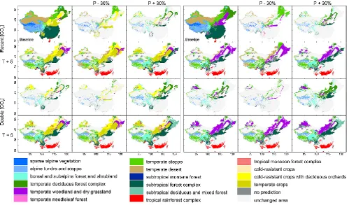
Results of the sensitivity experiments are shown in Fig. 5. In-creasing temperature by 5 K shifts the predicted boundaries of most vegetation types northward and westward. Tropical monsoon rainforest is predicted to occupy a large area in south China and a small area in the Sichuan Basin. Across the greater part of the Tibetan Plateau, alpine tundra and steppe are predicted to be replaced by temperate steppe in the south and in the north, and the temperate deciduous forest com-plex, boreal and subalpine forest and shrubland in the east. In this scenario, cold-resistant crops and deciduous orchards become suitable for planting along the river valleys in the southern part of the plateau.
Fig. 5. Changes in predicted vegetation distribution at projected scenarios, with a reference distribution at the baseline scenario (left panels for both natural and agriculture vegetation types, right panels only for natural vegetation type).
northeast–southwest axis where the current precipitation is at intermediate levels. In the southern (high-elevation) part of this axis, increased precipitation causes alpine tundra and steppe to give way to boreal and subalpine forest while spreading slightly northward into the area currently occu-pied by alpine sparse vegetation. In the northern part of this axis, increased precipitation benefits the mesic vegetation (boreal and subalpine forest and shrubland, the temperate de-ciduous forest complex, temperate woodland and dry grass-land) at the expense of xeric vegetation (temperate steppe, temperate desert). The effects of decreasing precipitation are broadly opposite to the effects of increasing precipitation. In-creased precipitation also leads to more heterogeneous veg-etation on the Loess Plateau, with temperate woodland and dry grassland, temperate needleleaf forest and a temperate deciduous forest mosaic all widely distributed. In the rest of China, where precipitation is either very low or high, the veg-etation distribution responds to precipitation changes much less strongly. The boundaries of tropical forest and temper-ate desert remain almost the same whether precipitation is increased or decreased, while the northern boundary of the subtropical forest complex shifts slightly to the north or to the south.
[CO2] doubling is estimated to have effects similar to
those of increasing precipitation by 30 %, favouring more
woody vegetation in the forest–grassland transition region (Fig. 5). In the temperate zone, [CO2] doubling produces a
shift from temperate steppe to temperate woodland and dry grassland, and to temperate deciduous forest complex. On the Tibetan Plateau, [CO2] doubling favours boreal and
sub-alpine forest and shrubland over sub-alpine tundra and steppe.
4 Discussion
4.1 Comparison with previously published results
BIOME4 overestimates the distribution area of temperate steppe at the expense of temperate forest. By refining the categories of forest vegetation, the empirical model also pro-vides more detailed information about the most economically productive semi-natural vegetation in China. Most impor-tantly, the ability of the empirical model to predict cropland distributions points towards a way to assess the changing suitability of agricultural systems under scenarios of changes in climate and [CO2].
As also shown by BIOME4, the transition region between mesic and xeric vegetation along a northeast–southwest axis is the region most likely to experience major vegetation changes as a result of climate change. Warming is gener-ally expected to favour woody vegetation there. The effects depend on the trajectory of precipitation changes; without an increase in precipitation, some regions suffer drought and thus a decline in forests. However the positive effect seems much stronger than the negative one, since water limitation is not severe in the majority of this region. On the Tibetan Plateau, where energy is the key limitation for woody plants, boreal and subalpine forest and shrubland are predicted to expand in response to warming, causing alpine tundra and steppe to retreat westward. In the central part, temperate woodland and dry grassland tend to expand at the expense of temperate steppe, while the subtropical forest complex ex-pands at the expense of temperate woodland. In semi-arid re-gions in the north, warming benefits temperate woodland and dry grassland at the expense of temperate steppe, but also temperate steppe expands into the current distribution area of the temperate deciduous forest complex, due to drought. Changes in plant water availability, either directly due to changes in precipitation or indirectly due to [CO2]-induced
changes in water use efficiency, are predicted to modify the effects of warming by influencing the competition between woody and herbaceous plants.
The Tibetan Plateau is identified both here and in the ear-lier study with BIOME4 as a region liable to experience large changes in vegetation as a result of climate change. Both models predict that warming will cause alpine vegeta-tion to retreat to the colder and drier areas toward the north. But BIOME4 suggests that alpine vegetation will be replaced mainly by forests, while the empirical model suggests that it will be replaced by temperate steppe. The vegetation around the eastern edge of the plateau was predicted by BIOME4 as being quite resistant to precipitation changes, but our new empirical model identifies this region as particularly sensitive to precipitation changes.
The present study indicates that the northern boundary of the tropical monsoon forest complex would move northward by as much as 4◦of latitude and even emerge in the Sichuan Basin. BIOME4 did not show this movement, probably be-cause of the strong minimum temperature constraint ap-plied to tropical forests in that model. The northward move-ment predicted here is probably more realistic than the stasis shown by BIOME4.
The empirical model makes no prediction about the veg-etation on the North China Plain when temperature increase is combined with precipitation decrease under recent [CO2].
This is the most severe scenario for mesic vegetation. The region in question was identified as a sensitive area by BIOME4, which predicted a transition to grassland and dry shrubland. The empirical model makes no prediction because the climate under this scenario is outside the range that the empirical models could predict based on current observa-tions. The actual vegetation is temperate croplands, which are adapted to the climate with the help of irrigation. How-ever, the North China Plain is one of the most water-scarce regions in the world (having less than half the water availabil-ity per person than water-scarce Egypt, in relation to its pop-ulation). The observed warmer and drier climate over the last four decades, combined with increasing water requirements both for industrial production and in daily life, has already exerted considerable pressure on irrigation systems. Most cli-mate models suggest that precipitation should increase in this region, but this is not certain and not predicted by all models (Cruz et al., 2007). Thus irrigated agriculture in the North China Plain represents a potential area of vulnerability to changes in climate and water supply.
4.2 The climate sensitivity of agriculture
By including crops in our analysis, we could investigate climate-dependent shifts in agricultural zones. Generally, warming is projected to shift agricultural zones significantly northward. This is directly demonstrated for the major crop-ping systems in north China, and implicitly indicated by the projected shift of natural vegetation types that include some agricultural types. These findings are consistent with data from the Chinese National Bureau of Statistics (2009) showing that, during the period from the early 1980s to 2007, warming enabled a significant northward expansion of rice planting in the northernmost region, between 48 and 52◦N. By 2007 the planted area of winter wheat in northern China moved northward by nearly 100 km compared with the 1960s. Paddy rice, the new dominant crop in the origi-nal corn-planting areas, has greatly expanded in Heilongjiang Province (Li and Wang, 2010). However, our analysis also points to the strong dependence of the cropland area in north China on precipitation, and the importance of irrigation re-quirements that could be limited by water supply. Unlike rainfed crops, decreased runoff with climate change could become an important limitation for the shift of irrigated crops in some areas.
Agricultural systems that were included in natural vegeta-tion classes showed relatively minor responses to precipita-tion change, with one excepprecipita-tion: “one crop annually short growing period cold-resistant crops”, which was included in the temperate deciduous forest complex. The effects of [CO2] on crop distribution cannot realistically be assessed
would be via the total increase of C3 crop productivity due
to CO2fertilization as well as water saving, rather than the
effects of enhanced water use efficiency mediated by compe-tition.
Topography could limit agricultural expansion. Although crops are predicted by the model in the Yungui Plateau, and their area of suitability predicted to expand, the actual veg-etation there today is forest. This area is well known for its karst topography which makes agriculture difficult.
4.3 Regional variations in the response to uniform perturbations of climate and [CO2]
According to projected climate trends summarized in Cruz et al. (2007), warming over all of China is likely to be greater during winter than summer, and the warming is likely to be especially strong on the Tibetan Plateau and in semi-arid regions. Mean precipitation will likely increase in most of China but decrease in some western areas. Thus, woody veg-etation will be favoured by future climate, as well as by el-evated [CO2]. In other words, forests with their important
functions in carbon sequestration, water retention and high biodiversity will likely continue to be the predominant nat-ural vegetation cover in a large area of China, and the area suitable for forests is likely to expand into regions currently occupied by grasslands. The Tibetan Plateau and some in-land desert areas are projected to experience large vegetation changes.
4.4 Caveats
The prediction skill of our empirical model for the present climate is inevitably highly reliant on the accuracy of the gridded climate data used to develop and run the model. One problematic region is the lower-elevation area to the south-east of the Tibetan Plateau (Zangnan area, a disputed territory between China and India) where the gridded climate data are not well constrained by observations. This data problem is probably the cause of the model’s underestimation of trop-ical rainforest in this region, and means that the projection of climate change effects here should be treated with scepti-cism.
Here, we have shown results of climate change in the form of stylized sensitivity experiments, rather than plausi-ble scenarios of the future. The idea was to understand how a uniform perturbation of climate would affect vegetation pat-terns. It remains to be seen how realistic climate change sce-narios, derived from climate models, translate into projected effects on ecosystems in China. Realistic scenarios include additional regional variations – in the climate changes them-selves – and in particular, the whole region is not predicted to get uniformly drier or wetter; but rather some areas are pre-dicted to get drier and some wetter. Only [CO2] is expected
to change uniformly across the country. Another study has applied future climate change projections derived from a set
of seven global climate model outputs, to assess likely di-rections of change in vegetation distribution and productivity during the 2070s (Wang 2013).
Due to the equilibrium assumption, the approach we ap-plied here entails some unavoidable limitations. The fitted empirical models do not predict when changes in vegeta-tion are likely to happen. The predicted responses of veg-etation distributions to climate could be achieved in reality only some decades to centuries after the new climate state has been established. Also, since we focused on the primary con-trols of mean climatic conditions on large-scale patterns of vegetation distribution, processes related to vegetation suc-cession and migration, such as fire disturbances and dispersal constraints, are not modelled. But despite these limitations, the method described here makes good use of extensive ob-servational data sets applying to the specific region of inter-est. The results should therefore be a reliable guide to the general direction and magnitude of changes to be expected in the region in response to the prescribed scenarios of change in [CO2] and climate.
Supplementary material related to this article is available online at: http://www.biogeosciences.net/10/ 5817/2013/bg-10-5817-2013-supplement.pdf.
Acknowledgements. This work was supported by a National Basic Research Program of China grant (2010CB951303) and an award to J. Ni from the One Hundred Talents Program of the Chinese Academy of Sciences. We thank the China Scholarship Council (CSC) and Macquarie University for supporting H. Wang to study at Macquarie.
Edited by: V. Brovkin
References
Antle, J., Apps, M., Beamish, R., Chapin, T., Cramer, W., Frangi, J., Laine, J., Erda, L., Magnuson, J., Noble, I., Price, J., Prowse, T., Root, T., Schulze, E., Sirotenko, O., Sohngen, B., and Sous-sana, J.: Ecosystems and Their Goods and Services, in: Climate Change 2001: Impacts, Adaptation and Vulnerability, Contribu-tion of Working Group II to the Third Assessment Report of the Intergovernmental Panel on Climate Change, edited by: Mc-Carthy, J. J., Canziani, O. F., Leary, N. A., Dokken, D. J., and White, K. S., Cambridge University Press, Cambridge, 235–342, 2002.
Beaumont, L. J., Hughes, L., and Poulsen, M.: Predicting species distributions: use of climatic parameters in BIOCLIM and its im-pact on predictions of species, current and future distributions, Ecol. Model., 186, 251–270, 2005.
Bragg, F. J., Prentice, I. C., Harrison, S. P., Eglinton, G., Foster, P. N., Rommerskirchen, F., and Rullk¨otter, J.: Stable isotope and modelling evidence for CO2 as a driver of glacial-interglacial vegetation shifts in southern Africa, Biogeosciences, 10, 2001– 2010, doi:10.5194/bg-10-2001-2013, 2013.
Breheny, P. and Burchett, W.: Visreg: Visualization of Regression Models, R package version 2.0-0, URL http://CRAN.R-project. org/package=visreg, 2013.
Cohen, J.: A coefficient of agreement for nominal scales, Educ. Psy-chol. Meas., 20, 37–46, 1960.
Cruz, R. V., Harasawa, H., Lal, M., Wu, S., Anokhin, Y., Punsalmaa, B., Honda, Y., Jafari, M., Li, C., and Ninh, N. H.: Asia, in: Cli-mate Change 2007: Impacts, Adaptation and Vulnerability, Con-tribution of Working Group II to the Fourth Assessment Report of the Intergovernmental Panel on Climate Change, edited by: Parry, M. L., Canziani, O. F., Palutikof, J. P., van der Linden, P. J., and Hanson, C. E., Cambridge University Press, Cambridge, 469–506, 2007.
Easterling, W. E., Aggarwal, P. K., Batima, P., Brander, K. M., Erda, L., Howden, S. M., Kirilenko, A., Morton, J., Soussana, J.-F., Schmidhuber, J., and Tubiello, F. N.: Food, Fiber, and For-est Products, in: Climate Change 2007: Impacts, Adaptation and Vulnerability, Contribution of Working Group II to the Fourth Assessment Report of the Intergovernmental Panel on Climate Change, edited by: Parry, M. L., Canziani, O. F., Palutikof, J. P., van der Linden, P. J., and Hanson, C. E., Cambridge University Press, Cambridge, 273–313, 2007.
Gallego-Sala, A. V. and Prentice, I. C.: Blanket peat biome endan-gered by climate change, Nat. Clim. Change, 3, 152–155, 2013. Gallego-Sala, A. V., Clark, J. M., House, J. I., Orr, H. G., Prentice,
I. C., Smith, P., Farewell, T., and Chapman, S. J.: Bioclimatic envelope model of climate change impacts on blanket peatland distribution in Great Britain, Clim. Res., 45, 151–162, 2011. Hancock, P. A. and Hutchinson, M. F.: Spatial interpolation of large
climate data sets using bivariate thin plate smoothing splines, En-viron. Modell. Softw., 21, 1684–1694.
Harrison, S. P. and Prentice, I. C.: Climate and CO2controls on
global vegetation distribution at the last glacial maximum: anal-ysis based on palaeovegetation data, biome modeling and palaeo-climate simulations, Glob. Change Biol., 9, 983–1004, 2003. Harrison, S. P., Kutzbach, J. E., Liu, Z., Bartlein, P. J.,
Otto-Bliesner, B., Muhs, D., Prentice, I. C., and Thompson, R. S.: Mid-Holocene climates of the Americas: a dynamical response to changed seasonality, Clim. Dynam., 20, 663–688, 2003. Harrison, S. P., Prentice, I. C., Barboni, D., Kohfeld, K. E., Ni, J.,
and Sutra, J.-P.: Ecophysiological and bioclimatic foundations for a global plant functional classification, J. Veg. Sci., 21, 300– 317, 2010.
Hartigan, J. A. and Wong, M. A.: Algorithm AS 136: A K-Means Clustering Algorithm, J. Roy. Stat. Soc. C-App., 28, 100–108, 1979.
Howden, S. M., Reyenga, P. J., and Meinke, H.: Global change impacts on Australian wheat cropping – Report to the Aus-tralian Greenhouse Office, CSIRO Wildlife and Ecology, Can-berra, 1999.
Keenan, T. F., Maria Serra, J., Lloret, F., Ninyerola, M., and Sabate, S.: Predicting the future of forests in the Mediterranean under cli-mate change, with niche- and process-based models: CO2 mat-ters!, Glob. Change Biol., 17, 565–579, 2011.
Keenan, T. F., Hollinger, D. Y., Bohrer, G., Dragoni, D., Munger, J. W., Schmid, H. P., and Richardson, A. D.: Increase in forest water-use efficiency as atmospheric carbon dioxide concentra-tions rise, Nature, 499, 324–327, 2013.
Li, Y. and Wang, C.: Impacts of Climate Change on Crop Planting Structure in China, Adv. Clim. Change Res., 6, 123–129, 2010. Luo, T. X.: Patterns of net primary productivity for Chinese major
forest types and their mathematical models, Doctor of Philoso-phy, Chinese Academy of Sciences, Beijing, 1996.
Monserud, R. A.: Methods for comparing global vegetation maps, Working Paper WP-90-40International Institute for Applied Sys-tems Analysis, 31, 1990.
Pearson, R. G. and Dawson, T. P.: Predicting the impacts of climate change on the distribution of species: are bioclimate envelope models useful?, Global Ecol. Biogeogr., 12, 361–371, 2003. Peterson, A. T.: Predicting species’ geographic distributions based
on ecological niche modeling, Condor, 103, 599–605, 2001. Phillips, S. J., Anderson, R. P., and Schapire, R. E.: Maximum
entropy modeling of species geographic distributions, Ecol. Model., 190, 231–259, 2006.
Prentice, I. C. and Harrison, S. P.: Ecosystem effects of CO2
con-centration: evidence from past climates, Clim. Past, 5, 297–307, doi:10.5194/cp-5-297-2009, 2009.
Prentice, I. C., Cramer, W., Harrison, S. P., Leemans, R., Monserud, R. A., and Solomon, A. M.: A global biome model based on plant physiology and dominance, soil properties and climate, J. Bio-geogr., 19, 117–134, 1992.
Prentice, I. C., Sykes, M. T., and Cramer, W.: A simulation model for the transient effects of climate change on forest landscapes, Ecol. Model., 65, 51–70, 1993.
Prentice, I. C., Harrison, S. P., and Bartlein, P. J.: Global vegetation and terrestrial carbon cycle changes after the last ice age, New Phytol., 189, 988–998, 2011.
Prentice, I. C., Baines, P. G., Scholze, M., and Wooster, M. J.: Fun-damentals of Climate Change Science, in: Understanding the Earth System: Global Change Science for Application, edited by: Cornell, S. E., Prentice, I. C., House, J. I., and Downy, C. J., Cambridge University Press, 39–71, 2012.
Rosenzweig, C., Casassa, G., Karoly, D. J., Imeson, A., Liu, C., Menzel, A., Rawlins, S., Root, T. L., Seguin, B., and Try-janowski, P.: Assess- ment of observed changes and responses in natural and managed systems, in: Climate Change 2007: Impacts, Adaptation and Vulnerability, Contribution of Working Group II to the Fourth Assessment Report of the Intergovernmental Panel on Climate Change, edited by: Parry, M. L., Canziani, O. F., Pa-lutikof, J. P., van der Linden, P. J., and Hanson, C. E., Cambridge University Press, Cambridge, 79–131, 2007.
Rounsevell, M. D. A., Pedroli, B., Erb, K.-H., Gramberger, M., Busck, A. G., Haberl, H., Kristensen, S. r., Kuemmerle, T., Lavorel, S., Lindner, M., Lotze-Campen, H., Metzger, M. J., Murray-Rust, D., Popp, A., P´erez-Soba, M., Reenberg, A., Vadineanu, A., Verburg, P. H., and Wolfslehner, B.: Challenges for land system science, Land Use Policy, 29, 899–910, 2012. Rural Socio-Economic Survey Organization: National Bureau of
Statistics of China Agricultural Statistics from 1978 to 2007 (in Chinese), China Statistics Press, Beijing, 2009.
ter-restrial carbon cycle, future plant geography and climate-carbon cycle feedbacks using five Dynamic Global Vegetation Models (DGVMs), Glob. Change Biol., 14, 2015–2039, 2008.
Smith, M. J., Purves, D. W., Vanderwel, M. C., Lyutsarev, V., and Emmott, S.: The climate dependence of the terrestrial carbon cycle, including parameter and structural uncertainties, Biogeo-sciences, 10, 583–606, doi:10.5194/bg-10-583-2013, 2013. Sykes, M. T., Prentice, I. C., and Cramer, W.: A bioclimatic model
for the potential distributions of north European tree species un-der present and future climates, J. Biogeogr. 23, 203–233, 1996. Ter Braak, C. J. F. and Prentice, I. C.: A Theory of Gradient
Analy-sis, Adv. Ecol. Res., 18, 271–331, 1998.
Wang, H.: A multi-model assessment of climate change impacts on the distribution and productivity of ecosystems in China, Reg. Environ. Change, doi:10.1007/s10113-013-0469-8, 2013. Wang, H., Ni, J., and Prentice, I. C.: Sensitivity of potential natural
vegetation in China to projected changes in temperature, precip-itation and atmospheric CO2, Reg. Environ. Change, 11, 715–
727, 2011.
Wang, H., Prentice, I. C., and Ni, J.: Primary production in forests and grasslands of China: contrasting environmental responses of light- and water-use efficiency models, Biogeosciences, 9, 4689– 4705, doi:10.5194/bg-9-4689-2012, 2012.