Kinetic bottlenecks to respiratory exchange rates in the deep-sea – Part 1: Oxygen

(1)

Biogeosciences, 10, 5049–5060, 2013 www.biogeosciences.net/10/5049/2013/ doi:10.5194/bg-10-5049-2013

EGU Journal Logos (RGB)

Advances in

Geosciences

Open Access

Natural Hazards

and Earth System

Sciences

Open Access

Annales

Geophysicae

Open Access

Nonlinear Processes

in Geophysics

Open Access

Atmospheric

Chemistry

and Physics

Open Access

Atmospheric

Chemistry

and Physics

Open Access Discussions

Atmospheric

Measurement

Techniques

Open Access

Atmospheric

Measurement

Techniques

Biogeosciences

Open Access Open Access

Biogeosciences

Discussions

Climate

of the Past

Climate

of the Past

Discussions

Earth System

Dynamics

Earth System

Dynamics

Discussions

Geoscientific

Instrumentation

Methods and

Data Systems

Open Access

_{Geoscientific}

Instrumentation

Methods and

Data Systems

Geoscientific

Model Development

Geoscientific

Model Development

Discussions

Hydrology and

Earth System

Sciences

Open Access

Hydrology and

Earth System

Sciences

Ocean Science

Discussions

Solid Earth

Discussions

The Cryosphere

Discussions

Natural Hazards

and Earth System

Sciences

Open Access

Discussions

Kinetic bottlenecks to respiratory exchange rates in the deep-sea –

Part 1: Oxygen

A. F. Hofmann1,2, E. T. Peltzer1, and P. G. Brewer1

1_{Monterey Bay Aquarium Research Institute (MBARI), 7700 Sandholdt Road, Moss Landing, CA 95039-9644, USA} 2_{German Aerospace Center (DLR), Institute of Technical Thermodynamics, Pfaffenwaldring 38–40, 70569 Stuttgart,}

Germany

Correspondence to: A. F. Hofmann (andreas.hofmann@dlr.de)

Received: 9 September 2012 – Published in Biogeosciences Discuss.: 11 October 2012 Revised: 14 June 2013 – Accepted: 25 June 2013 – Published: 25 July 2013

Abstract. Ocean warming is now reducing dissolved

oxy-gen concentrations, which can pose challenges to marine life. Oxygen limits are traditionally reported simply as a static concentration threshold with no temperature, pressure or flow rate dependency. Here we treat the oceanic oxygen supply potential for heterotrophic consumption as a dynamic molecular exchange problem analogous to familiar gas ex-change processes at the sea surface. A combination of the purely physico-chemical oceanic properties temperature, hy-drostatic pressure, and oxygen concentration defines the abil-ity of the ocean to provide the oxygen supply to the external surface of a respiratory membrane. This general oceanic oxy-gen supply potential is modulated by further properties such as the diffusive boundary layer thickness to define an upper limit to oxygen supply rates. While the true maximal oxygen uptake rate of any organism is limited by gas transport ei-ther across the respiratory interface of the organism itself or across the diffusive boundary layer around an organism, con-trolled by physico-chemical oceanic properties, it can never be larger than the latter. Here, we define and calculate quanti-ties that describe this upper limit to oxygen uptake posed by physico-chemical properties around an organism and show examples of their oceanic profiles.

1 Introduction

One of the challenges facing ocean science is the need to make a formal connection between the emerging changes in the physico-chemical properties of the ocean, such as rising temperature and CO2levels and declining O2, and the

phys-ical combination of these properties that best describes the external boundary condition for the rate at which O2can be

transported across membrane surfaces. Here, we focus on the theoretical background for characterization, description, and mapping of the impacts of ocean deoxygenation from a gas exchange rate perspective.

The rate controls of diffusive processes are well under-stood and embodied in Fick’s First Law. The solubility of the metabolically important gases is well known as a function of salinity and temperature (Weiss, 1970, 1974; Garcia and Gor-don, 1992). From this and the observed distributions, partial pressures can be calculated. Likewise, the diffusion coeffi-cients of the substances in question and their variation with temperature, as well as generally accepted formulations of the linkages between boundary layer thickness and fluid flow, are known. From these fundamental principles and observa-tions, one can derive combined quantities which embody the essential chemical and physical principles in useful ways to illustrate and predict future changes in the ocean.

The quantities we define here are meant to be used in physico-chemical models of the ocean, for mapping the changing O2 supply capacity of areas of interest such as

(2)

2 Oceanic oxygen supply: physico-chemical vs. organism-specific quantities

The O2demands of marine organisms have classically been

described as a rate problem (e.g. Hughes, 1966) in which diffusive transport across a boundary layer driven by partial pressure differences takes place. As with gas exchange rates at the sea surface (e.g. Wanninkhof, 1992) where wind speed is a critical variable, bulk fluid flow velocity over the animal surface is important. An oxygen concentration value alone does not adequately describe this process. For example, giv-ing only an oxygen concentration as a limit for oxygen sup-ply specifies no temperature-dependent information, so that the same value is assumed to be limiting over a temperature span of possibly 30◦C. This can be overcome to some ex-tent by providingpO2as a limiting value (Hofmann et al.,

2011), but the rate problem for gas transfer across a diffusive boundary layer contains also terms for diffusivity, and the relationship between boundary layer thickness and velocity over the surface, and thus a much more complete description would be useful.

The challenge in defining generic properties that describe the ocean in a way that is relevant to generic membrane trans-port of O2is to separate as best as possible the purely

phys-ical terms which are universally applicable, such as temper-atureT, oxygen concentration [O2], hydrostatic pressureP

(together resulting in an oxygen partial pressurepO2),

dif-fusivity (resulting from salinityS,T, andP), and the basic fluid dynamical form of the dependence of boundary thick-ness on flow.

There is no debate over the T, [O2], P, and

diffusiv-ity terms since these are fundamental, organism-independent ocean chemical properties. The difficulty is in providing a way of including the flow term as a generic, organism-independent principle. There is no doubt of the existence of a diffusive boundary layer that is present over all ocean sur-faces, thus also over all respiratory gas exchange interfaces. Generic and simplified descriptions of boundary layers are essential and widely used also for air–sea gas exchange rates, mineral dissolution rates, and phytoplankton nutrient uptake rates. The most widely used formulation is based on the dimensionless Schmidt number (e.g. Santschi et al., 1991; Wanninkhof, 1992). This relationship is standard within the ocean sciences and physiology (e.g. Pinder and Feder, 1990) and is also used here based on a planar surface model for the molecular exchange surface, which works well for all but microscopic scales (Zeebe and Wolf-Gladrow, 2001). We de-rive all gas flux properties on a per-square-centimeter scale so as to provide a way to normalize for different respiratory surface areas.

We stress that the end result desired is to provide improved functions and profiles that better allow comparison between different ocean regions undergoing change in their oxygen supply potential as the ocean warms and O2levels decline.

3 Materials and methods

A list of symbols and abbreviations used throughout this pa-per can be found in Table 1.

3.1 The oceanic oxygen supply potential SPO2

Here we define the oceanic oxygen supply potential as the combination ofpO2and diffusivity under in situ conditions

constituting a theoretical maximal upper limit for respiratory O2uptake as provided by a given oceanic region.

Respiratory gas molecules expelled or taken up have to tra-verse both the respiratory interface and the diffusive bound-ary layer (DBL) in the medium surrounding the respiratory interface on the outside, i.e. the surrounding ocean. In gen-eral, either one of these steps can be the rate-limiting step for respiratory gas transport (see also the companion paper: Hofmann et al., 2013).

We denoteEDBLas the maximal diffusive oxygen flux if

only the diffusive boundary layer would need to be traversed (hypothetically assuming insignificant respiratory interface barrier). And Eint as the maximal diffusive oxygen flux if

only the respiratory interface would need to be traversed (hy-pothetically assuming insignificant boundary layer barrier). We can then write for the true total diffusive flux of oxygen

E(in µmol O2s−1cm−2) into an animal across both barriers

E≤min(Eint, EDBL) , (1)

which means the diffusive flux across both barriersEis al-ways smaller than or equal to the maximal flux that the DBL transversion permits (i.e.EDBL), and we can write

E≤EDBL. (2)

EDBL, however, can be expressed by the standard represen-tation (e.g. Santschi et al., 1991; Boudreau, 1996; Zeebe and Wolf-Gladrow, 2001) of Fick’s First Law, using gas partial pressures (e.g. Piiper, 1982; Feder and Burggren, 1985; Pin-der and Burggren, 1986; PinPin-der and FePin-der, 1990; Maxime et al., 1990; Pelster and Burggren, 1996) as1

EDBL= D ρSW

L K00 1pO2|DBL. (4) 1_where_ρ

SW is the in situ density of seawater (calculated

ac-cording to Millero and Poisson (1981) as implemented in Hofmann et al. (2010)) in kg cm−3;Dis the molecular diffusion coefficient for O2in cm2s−1, calculated from temperature and salinity, e.g. as

given in Boudreau (1996, Chapter 4);Lis the DBL thickness in cm; 1pO₂|_DBLin µatm is the oxygen partial pressure difference across the DBL; and whereK00is the apparent Henry’s constant for O2in

mol kg−1atm−1(= µmol kg−1µatm−1) at in situ conditions:

K00= [O2]

pO₂([O₂], T , S, P ), (3)

where [O2] in mol kg−1here is the O2concentration and in the

(3)

[image:3.595.43.545.79.488.2]

Table 1. List of symbols and abbreviations – listed in the order of their appearance in the manuscript.

Symbol Unit Meaning

[O2] µmol kg−1 oxygen concentration

pO2 µatm oxygen partial pressure

S salinity

T K or◦C bulk oceanic temperature

P bar (hydrostatic) pressure

DBL diffusive boundary layer around the gas exchange interfaces

EDBL µmol s−1cm−2 hypothetical diffusion-only oxygen uptake rate per area of gas exchange interface if only

the DBL was to cross, hypothetically assuming no respiratory interface barrier

Eint µmol s−1cm−2 hypothetical diffusion-only oxygen uptake rate per area of gas exchange interface if only

the respiratory interface was to cross, hypothetically assuming no DBL over the exchange surface

E µmol s−1cm−2 true oxygen uptake rate per area of gas exchange interface across the DBL and the respiratory interface together

D cm2s−1 molecular diffusion coefficient for O2

ρSW kg cm−3 in situ density of seawater

L cm DBL thickness

K00 mol kg−1atm−1

(µmol kg−1µatm−1)

apparent Henry’s constant for O₂

K00_IS mol kg−1atm−1 apparent Henry’s constant for O₂at in situ conditions K00_E mol kg−1atm−1 apparent Henry’s constant for O₂at experimental conditions

pO2([O2], T , S, P ) atm in situ oceanic oxygen partial pressure as a function of carbon dioxide concentration,

temperature, salinity, and hydrostatic pressure

1pO2|DBL µatm O2partial pressure difference across the DBL

pO₂|_f µatm ambient free stream oxygen partial pressure (outside of the DBL)

pO2|s µatm oxygen partial pressure directly at the respiratory surface (outside of the organism, but

past the DBL)

SPO2 µmol s

−1_cm−1 _{oceanic O}

2supply potential (see text for explanations)

K cm s−1 mass transfer coefficient for O₂

u100 cm s−1 free stream fluid flow velocity over gas exchange surfaces

Emax µmol s−1cm−2 Maximal hypothetical oxygen uptake rate per area of gas exchange interface, as permitted

by DBL diffusion limitation

pf µatm minimalpO2|fthat is able to support a givenE(all other conditions remaining constant)

Cf µmol kg−1 minimal oxygen concentration [O2] that is able to support a givenE(all other conditions

remaining constant)

Combining Eqs. (2) and (4) results in

E≤D ρSW

L K00 1pO2|DBL. (5)

With this inequality, we can calculate an upper boundary for the diffusive flux of O2into an animal, as posed by the

bar-rier of the diffusive boundary layer and the localpO2in the

oceanic environment surrounding it. The true oxygen flux into an animal might be limited by respiratory interface

trans-and hydrostatic pressure, first calculated conventionally from the oxygen saturation concentration (Garcia and Gordon, 1992) using potential temperature (θ; Bryden, 1973; Fofonoff, 1977). Resulting pO2values are then corrected for hydrostatic pressure (calculated

from given depth values according to Fofonoff and Millard (1983)) according to Enns et al. (1965).

port2, but it is always lower than the upper boundary defined by the right-hand side of Eq. (5).

The oxygen partial pressure difference across the DBL

pO2|DBLcan be expressed as

1pO2|DBL=pO2|f−pO2|s, (6)

withpO2|fexpressing the oxygen partial pressure in the free

stream beyond the DBL and pO2|s expressing the oxygen

partial pressure directly on the gas exchange surface of the organism. Since, obviously,pO2|s≥0 atm, the following

in-equality always holds true:

1pO2|DBL≤pO2|f. (7) 2_{Interface transport limitation is an important and interesting}

(4)

Since our aim is to calculate an upper boundary for oxygen flux into an organism, we can simplify Eq. (5) by combining it with Eq. (7) to

E≤D ρSWK0

0

L pO2|f. (8)

Equation (8) expresses the fact that the true respiratory gas exchange per unit area of gas exchange surface is always smaller thanD ρSWK00

L pO2|f. This expression, however, con-tains the DBL thickness L, which is an organism-specific quantity as it depends on the unique surface microstructure of the respiratory surface area and any unique characteristics of the organism shape and mode of swimming or pumping. So, in order to arrive at a purely physico-chemical quantity that describes the organism-independent oceanic propensity for supplying oxygen, we multiply Eq. (8) byLand arrive at

E L≤D ρSWK00pO2|f. (9)

This allows us to define the oceanic oxygen supply poten-tial SPO2 in µmol s

−1_cm−1_{as the upper limit (i.e. maximal}

value) for the product of the respiratory oxygen uptake rate

Eand the DBL thicknessL.

SPO2:=D ρSWK0

0

pO2|f=D ρSW[O2]f (10)

Thus, SPO2 is a purely physical oceanic property, not

depen-dent on any organism-specific properties or characteristics. It can be used to generate profiles and maps that illuminate which regions of the ocean are better able to support aer-obic marine life than can simple O2 concentration profiles

or maps, since it incorporates the essentialT,P and further diffusion-related terms.

3.2 The generic maximal theoretical oxygen supply rate

Emax

All respiratory external surfaces will have a diffusive bound-ary layer that provides the contact with the ocean waters, and the thickness of this will in the macroscopic case3 depend upon the external flow over this surface, whether passive or controlled by organism motions. The most generic case is a simple planar surface description of the flow dependency ofL, as was used to describe the mineral dissolution exper-iments in Santschi et al. (1991): the DBL thickness Lcan be expressed as the fraction of the molecular diffusion co-efficientDand the mass transfer coefficient K, which is a function of the fluid flowu100.

L= D

K (u100), (11)

3_{In microscopic organisms,}_L_{is usually taken to be equal to the}

radius of the sphere of the microorganism (cf. e.g. Stolper et al., 2010) – in this case, our formulation forEmaxcan still be used with

the appropriateL.

which effectively makesLa function of flow velocityu100. Table 2 details this generic description ofLas a function of

u100.

For a given free stream oxygen partial pressurepO2|f,

sub-stituting Eq. (11) into Eq. (8) allows us to define an upper limit or for the oxygen uptake rateEper unit area of respira-tory interface supported by the givenpO2|fas

Emax:=SPO2

L =

D ρSWK00

L pO2|f. (12)

This definition ofEmaxas an upper limit for the oxygen up-take rate utilizes a simplified and generic model to describe

L.Emaxvalues are thus not biologically specific, but are in-tended solely to compare various oceanic regions in their

po-tential to supply oxygen under given in situ conditions and to

offer a rough estimate as to how flow rates over respiratory interfaces influence this potential.

3.3 The minimal oxygen concentrationCfsupporting a

given laboratory-determinedE

The traditional use of only the oxygen concentration [O2]

as a measure does not take into account the large regional variations inT,P, and further diffusion-related quantities, so it is useful to compare functions containing these properties with [O2] alone.

In order to explicitly describe and reveal the influence of temperature and diffusion while comparing various oceanic regions, warm and shallow, as well as deep and cold, to one another, we define another quantity in which we remove the effect of the oxygen content of the water. To explicitly in-clude the important dependence of gas exchange on partial pressure (e.g. Piiper, 1982; Pinder and Feder, 1990; Pel-ster and Burggren, 1996; Childress and Seibel, 1998; Seibel et al., 1999) and the dependency of partial pressure on hydro-static pressure (Enns et al., 1965), we assume a given oxy-gen uptake rateE(in µmol s−1cm−2– without loss of gen-erality we assume throughout the paper a generic value of

E=20×10−7µmol s−1cm−2), experimentally determined at diffusivitiesDand DBL thicknessesLequal to the respec-tive in situ values, but at one atmosphere. From Eq. (8) we can then determine a relation between the free stream oxy-gen partial pressurepO2|fand this given oxygen uptake rate Eas

pO2|f≥ L

D ρSWK00_E E, (13)

which shows thatpO2|fhas to be greater or equal to the

right-hand side of Eq. (13) to support the givenE. Again describ-ing a limitdescrib-ing condition, we definepfas the minimalpO2|f

that can supportEas

pf:= L

D ρSWK00_E

(5)

Table 2. Expressing the DBL thicknessLas a function of water flow velocity: a generic planar surface description.

The DBL thicknessLcan be expressed as the fraction of the temperature-dependent molecular diffusion coefficientD for O2 in

cm2s−1, calculated from temperature and salinity as given in Boudreau (1996, Chapter 4) using the implementation in the R package marelac (Soetaert et al., 2010), and the mass transfer coefficientK(Santschi et al., 1991; Boudreau, 1996):

L= D K.

Kcan be calculated for O₂from the water-flow-induced shear velocity u0in cm s−1and the dimensionless Schmidt number Sc for O2(as calculated by linearly interpolating two temperature-dependent formulations forS=35 andS=0 in Wanninkhof (1992) with

respect to given salinity):

K=a u0Sc−b,

with parametersaandb: Santschi et al. (1991):a=0.078,b= 2

3; Shaw and Hanratty (1977) (also given in Boudreau (1996)):a=

0.0889,b=0.704; Pinczewski and Sideman (1974) as given in Boudreau (1996):a=0.0671,b=2

3; Wood and Petty (1983) as given

in Boudreau (1996):a=0.0967,b= 7

10. Due to small differences we use averaged results of all formulations.

u0can be calculated from the ambient current velocity at 100 cm away from the exchange surfaceu100and the dimensionless drag

coefficient c100(Sternberg, 1968; Santschi et al., 1991; Biron et al., 2004):

u0=u100

√ c100.

c100is calculated from the water flow velocityu100as (Hickey et al., 1986; Santschi et al., 1991)

c100=10−3

2.33−0.0526|u100| +0.000365|u100|2

.

As mentioned above, in order to compare with standard con-ditions at one atmosphere, we assume laboratory experimen-tal conditions at one atmosphere, so the apparent Henry’s Law constantK00_E in Eqs. (13) and (14) is calculated with one atmosphere. To explicitly include the hydrostatic pres-sure dependency of partial prespres-sure, i.e. to obtain the oxygen concentration that would result inpf at in situ hydrostatic pressures, we have to convertpfto a concentration using an apparent Henry’s Law constantK00_IScalculated at in situ hy-drostatic pressure. Thus, we can defineCf, the minimum

oxy-gen concentration [O2] in µmol kg−1the free flowing stream

must have to sustainE, as

Cf:=pfK00IS= L D ρSW

K00_IS

K00_E E. (15) The inclusion of the ratio of the Henry’s Law constants at one atmosphere and at in situ pressures explicitly includes the pressure dependency of partial pressures, which makes

Cfa quantity that can be used to directly compare warm and shallow to cold and deep oceanic regions.

3.4 Example oceanographic data

AllT,S,P, and [O2] data for ocean profiles have been

ex-tracted from the Ocean Data View (Schlitzer, 2010) version of the World Ocean Atlas 2009 oxygen climatology (Gar-cia et al., 2010). Calculations have been performed in the

open-source programming language R (R Development Core Team, 2010).

4 Results and discussion

As noted above, warming of the ocean (Levitus et al., 2005; Lyman et al., 2010) is reducing the oxygen concentration via the solubility effect, decreasing ventilation due to increased stratification and increasing oxygen drawdown from micro-bial mineralization of organic matter. Thus global ocean oxy-gen concentrations are declining (Chen et al., 1999; Jenkins, 2008; Stramma et al., 2008; Helm et al., 2011), and the com-bined effects of T and O2 have an impact on aerobic

per-formance (e.g. Poertner and Knust, 2007). Yet at the same time, increased temperature enhances diffusion and results in increased gas partial pressures for the same concentrations, both of which enhance diffusive oxygen uptake rates. The properties we define above allow for a comparison of the rel-ative roles and impacts of these opposing changes in oceanic properties.

To illustrate our newly defined quantities, we have cho-sen a set of example stations from different ocean basins for comparative purposes. Table 3 provides a tabulation for the classical oxygen concentration ([O2]) hydrographic depth

(6)

Table 3. Depth profiles of [O2], SPO2,Emax, andCffor example stations around the world. Details on the tabulated quantities can be

found in the text. The units used are as follows: [O₂]: µmol kg−1; SP_O₂ : 10−7µmol kg−1s−1cm−1;Emax: 10−7µmol kg−1s−1cm−2;

Cf : µmol kg−1. For all locations we assume a constant flow velocity of u100= 2 cm s−1; more realistic flow profiles or

organism-specific descriptions of the DBL thickness Lcan be employed here. For Cf calculations we assume a generic constant value ofE=

20×10−7µmol s−1cm−2.TE= 5◦C andSE=34. NA indicates that values are not available for the respective depth. SC: Southern

Cali-fornia (120.5◦W, 29.5◦N); WP: Western Pacific (126.5◦E, 11.5◦N); CH: Chile (75.5◦W, 33.5◦S); WA: Western Africa (6.5◦E, 15.5◦S); BB: Bay of Bengal (87.5◦E, 18.5◦N); MD: Mediterranean (18.5◦E, 35.5◦N).

SC WP CH

depth [O2] SPO2 Emax Cf [O2] SPO2 Emax Cf [O2] SPO2 Emax Cf

0 239 46 221 16.72 225 46 227 14.73 196 48 262 9.76

50 246 46 218 17.80 235 44 211 17.46 200 49 264 9.88

100 230 40 183 20.75 226 41 192 18.81 198 46 245 10.73

200 143 22 96 26.41 211 37 176 19.14 176 33 161 16.66

300 85 13 54 28.57 202 36 167 19.20 135 22 98 23.22

400 44 6 26 30.17 199 35 162 19.20 91 14 58 27.35

500 23 3 13 31.27 193 34 157 19.15 78 11 47 29.65

600 16 2 9 32.06 188 33 152 19.05 90 13 52 30.65

700 15 2 9 32.62 187 33 151 18.90 96 14 55 31.46

800 18 3 10 33.07 184 32 148 18.72 94 13 53 31.92

900 22 3 12 33.35 185 32 148 18.53 92 13 50 32.50

1000 28 4 15 33.63 185 32 148 18.33 94 13 51 32.79

1100 32 4 17 33.81 186 32 149 18.11 96 13 51 33.18

1200 36 5 19 33.90 190 33 152 17.88 94 13 50 33.38

1300 41 6 21 33.95 185 32 148 17.66 101 14 52 33.61

1400 46 6 24 33.97 190 33 152 17.44 102 14 52 33.76

1500 53 7 27 33.93 181 31 144 17.20 108 14 55 33.73

2000 82 11 40 33.37 192 33 153 16.11 115 15 57 33.02

3000 118 15 56 29.99 183 32 147 14.06 142 18 68 30.11

4000 132 17 63 26.22 190 33 152 12.29 152 20 72 26.27

WA BB MD

depth [O2] SPO2 Emax Cf [O2] SPO2 Emax Cf [O2] SPO2 Emax Cf

0 245 45 214 18.29 222 46 233 13.88 204 50 268 9.97

50 230 41 191 19.59 169 33 160 16.10 165 39 207 10.66

100 185 31 139 22.56 80 14 65 20.05 40 8 42 13.53

200 76 12 53 24.91 58 10 43 22.73 14 2 11 19.97

300 46 7 30 26.79 40 6 28 24.94 15 2 11 22.79

400 91 13 56 29.19 45 7 29 27.19 15 2 10 23.83

500 157 23 92 31.23 60 9 37 29.24 16 2 11 24.59

600 195 27 110 32.34 78 11 45 30.98 17 3 11 25.35

700 184 26 102 33.03 96 14 54 32.19 22 3 14 26.08

800 154 21 84 33.44 120 17 65 33.06 25 4 16 26.74

900 134 18 72 33.89 135 18 72 33.53 32 5 20 27.42

1000 123 17 65 34.11 146 20 78 33.62 40 6 24 28.09

1100 114 15 59 34.21 153 21 81 33.48 44 6 26 28.65

1200 112 15 58 34.20 166 22 87 33.22 50 7 29 29.19

1300 110 15 56 34.18 175 24 92 32.87 55 8 31 29.66

1400 112 15 57 34.13 188 25 98 32.52 67 9 37 30.16

1500 115 15 58 34.04 199 27 104 32.17 75 10 40 30.47

2000 134 17 66 33.06 220 30 113 30.90 106 14 53 32.05

3000 152 20 73 29.64 225 30 112 28.19 NA NA NA NA

[image:6.595.83.511.174.699.2]

(7)

example stations around the world ocean and the Mediter-ranean (SC: Southern California (120.5◦_{W, 29.5}◦_{N); WP:}

Western Pacific (126.5◦_{E, 11.5}◦_{N); CH: Chile (75.5}◦_W,

33.5◦S); WA: Western Africa (6.5◦E, 15.5◦S); BB: Bay of Bengal (87.5◦E, 18.5◦N); MD: Mediterranean (18.5◦E, 35.5◦N)).

4.1 Describing the oxygen supply potential of the ocean

including temperature effects: [O2] vs. SPO2

The leftmost column per station in Table 3 and Fig. 1 (both panels) show classical oxygen concentration profiles, and the second column in Table 3 and Fig. 2 show depth profiles of our newly defined oxygen supply potential SPO2 (Eq. 10).

It can be clearly seen that, while the general shape of the profiles is similar due to the dominating oxygen signal, there are marked differences in the overall range and especially at depth.

Those differences can be attributed to the effect of temperature-dependent diffusivity that is included in the defi-nition of SPO2. For example, while the oxygen concentration

increases again to about 60 % of surface values at 4000 m depth for the three Pacific Ocean stations shown (left panel, Fig. 1), SPO2values (left panel, Fig. 2) increase only to about

40 % of surface values due to colder temperatures limiting diffusion at depth. Similarly, the right panels of Figs. 1 and 2 show that, while the oxygen concentration at the Western Africa station rises above Mediterranean values at a depth of about 1500 m (Fig. 1), SPO2 values remain higher in the

Mediterranean all the way down to 4000 m depth (Fig. 2) due to diffusivity-enhancing higher temperatures. In the profiles shown for the station off Chile (CH, left panels of Figs. 1 and 2), the well-known horizontal penetration of an oxygen maximum into the oxygen minimum zone (Wyrtki, 1962) is reflected in the calculated SPO2 values; however, the local

maximum is less pronounced for SPO2 than for [O2] due to

the effect of temperature. The sample station in the Mediter-ranean (MD, right panels of Figs. 1 and 2), where there is a combination of the least diffusive restriction due to higher temperatures and a mean oxygen concentration being nearly twice as high as the site examined off Southern California (212 vs. 114 µmol kg−1), results in the highest deep water oxygen supply potential (SPO2) values for locations we have

examined. At the Bay of Bengal station (BB, right panel of Fig. 2), the waters at 800 m and below have a higher oxygen supply potential than the Southern California (SC) station, but at shallower depths the situation is reversed.

4.2 Incorporating a generic description of the influence of fluid flow velocity on dissolved gas exchange:

Emax

The quantityEmax(Eq. 12, Fig. 3, third column per station

in Table 3) determines the combined influences of oxygen concentration, temperature, and fluid flow velocity over gas

0 50 100 150 200 250

4000

3000

2000

1000

0

0 50 100 150 200 250

4000

3000

2000

1000

0

0 50 100 150 200 250

4000

3000

2000

1000

0

0 50 100 150 200 250 0 50 100 150 200 250 0 50 100 150 200 250 0 50 100 150 200 250

d

ep

th

/

m

SC

SC WA

BB MD WP

CH

[O2] /µmol kg−1

Fig. 1. [O2] depth profiles of the water column at different

hy-drographical stations around the world (SC: Southern California (120.5◦W, 29.5◦N); CH: Chile (75.5◦W, 33.5◦S); WP: West-ern Pacific (126.5◦E, 11.5◦N), WA: Western Africa (6.5◦E, 15.5◦S), MD: Mediterranean (18.5◦E, 35.5◦N); BB: Bay of Ben-gal (87.5◦E, 18.5◦N)).

exchange surfaces, so as to provide an estimate of the maxi-mal diffusive transport rates per unit gas exchange area that the ocean can support. Using a canonical constant mean flow over the animal respiratory surface ofu100= 2 cm s−1we can visualize example profiles of our quantityEmaxat our exam-ple stations in the world oceans (Fig. 3), which are, due to the constantu100, very similar in shape to the SPO2 profiles

in Fig. 2. To calculateEmaxvalues and profiles for specific purposes, detailed flow fields and organism-specific descrip-tions for the DBL thicknessLshould be used or more spe-cific molecular exchange models employed (see, e.g., Lazier and Mann, 1989; Karp-Boss et al., 1996). Here, we define

Emaxwith a generic description of its dependency onLand

thus fluid flow velocityu100.

[image:7.595.310.550.62.242.2]

(8)

10 20 30 40 50

4000

3000

2000

1000

0

10 20 30 40 50

4000

3000

2000

1000

0

10 20 30 40 50

4000

3000

2000

1000

0

10 20 30 40 50

d

ep

th

/

m

SC

SC WA

BB MD WP

CH

SPO2/ 10− 7

[image:8.595.50.290.60.243.2]

µmol s−1_cm−1

Fig. 2. Oxygen supply potential SP_O₂ depth profiles of the wa-ter column at different hydrographical stations around the world (SC: Southern California (120.5◦W, 29.5◦N); CH: Chile (75.5◦W, 33.5◦S); WP: Western Pacific (126.5◦E, 11.5◦N), WA: Western Africa (6.5◦E, 15.5◦S), MD: Mediterranean (18.5◦E, 35.5◦N); BB: Bay of Bengal (87.5◦E, 18.5◦N)).

physical formalism is the same. The limit case ofu100→0

would yieldL→ ∞. This example formulation forL as a function ofu100is thus not defined in a physically

meaning-ful way for zero flow velocity and should not be used for the stagnant water case. Here we plotLwith a minimum of

u100= 0.5 cm s−1, which can be seen as an operational lower limit.

4.3 Revealing the separate influences of temperature,

flow, and hydrostatic pressure on gas exchange:Cf

To explicitly single out the influence of temperature and fluid flow on gas exchange, which is co-mingled with the oxy-gen signal in profiles of SPO2 andEmax, and to additionally

incorporate the effect of hydrostatic pressure when compar-ing various oceanic regions in their ability to support given laboratory-determined respiratory ratesE, we have defined the quantity Cf. Cf profiles can then be compared to [O2]

profiles to determine oceanic regions that support the given oxygen demandE.

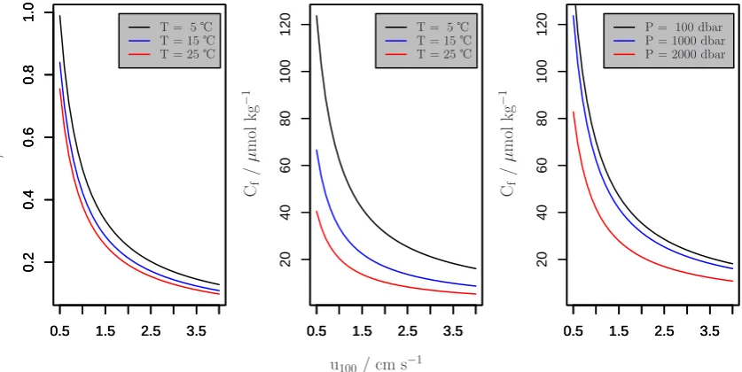
Due to the nonlinear dependency of the thickness of the diffusive boundary layerLon the current velocityu100, the minimal oxygen concentrationCf supporting a given oxy-gen uptake rateEis also a nonlinear function ofu100. The middle panel of Fig. 4 explicitly visualizes this dependency for different temperatures but constant pressure and salinity, and the right panel of Fig. 4 depicts this dependency for dif-ferent hydrostatic pressures. The left panel of Fig. 5 shows depth profiles ofCffor the SC example hydrographical

sta-tion (i.e. with in situ temperature, salinity and pressure) for three different values foru100. This further illustrates the

sen-sitivity ofCfwith respect tou100.

0 50 100 150 200 250

4000

3000

2000

1000

0

0 50 100 150 200 250

4000

3000

2000

1000

0

0 50 100 150 200 250

4000

3000

2000

1000

0

0 50 100 150 200 250 0 50 100 150 200 250 0 50 100 150 200 250 0 50 100 150 200 250

d

ep

th

/

m

SC

SC WA

BB MD WP

CH

[image:8.595.311.546.62.243.2]

Emax/ 10−7_µ_{mol s}−1_cm−2

Fig. 3. Generic maximal theoretical oxygen supply rateEmaxdepth

profiles of the water column at different hydrographical stations around the world (SC: Southern California (120.5◦W, 29.5◦N); CH: Chile (75.5◦W, 33.5◦S); WP: Western Pacific (126.5◦E, 11.5◦N), WA: Western Africa (6.5◦E, 15.5◦S), MD: Mediter-ranean (18.5◦E, 35.5◦N); BB: Bay of Bengal (87.5◦E, 18.5◦N))). A generic flow velocity ofu100= 2 cm s−1is assumed for all depths

to calculateL. If available, detailed flow profiles can be used here, as well as organism-specific descriptions forL.

It can be shown for the range ofu100 values in the mid-dle panel of Fig. 4, that a u100 decrease by half results in approximately a doubling ofCf (i.e.Cfis roughly propor-tional to the inverse ofu100). The nonlinear character of the relation between the fluid flow velocityu100and the limit for free stream oxygen concentrationCf is such that there is a low dependency whenu100>2 cm s−1and very high

depen-dency whenu100<1 cm s−1. This is a result of the respective

behavior of the thickness of the diffusive boundary layerL

onu100, as also described by, e.g., Garmo et al. (2006).

The right panel of Fig. 5 shows example depth profiles of

Cfat the SC station for three different respiratory ratesE, on

realistic orders of magnitude, to express the sensitivity ofCf

with respect toE.

The general shape ofCf depth profiles in Fig. 5 can be explained by comparison ofCf(Eq. 15) with its direct prede-cessor quantitypf(Eq. 14), the minimal oxygen partial pres-sure required to supportE. The quantityCfdirectly includes effects of diffusivity, boundary layer thickness, and tempera-ture and hydrostatic pressure effects on partial pressure. The predecessor quantitypfexpresses only effects on diffusivity

and boundary layer thickness. As temperature decreases with depth, so does the “efficiency“ of diffusion, with the result thatLincreases. This translates into a higherpfwith depth,

i.e. a higher necessarypO2to sustain the given oxygen

con-sumption rateE. The limit for oxygen concentrationCf

(9)

0.5 1.5 2.5 3.5

0.2

0.4

0.6

0.8

1.0

0.5 1.5 2.5 3.5

0.2

0.4

0.6

0.8

1.0

0.5 1.5 2.5 3.5

0.2

0.4

0.6

0.8

1.0

0.5 1.5 2.5 3.5

20

40

60

80

100

120

0.5 1.5 2.5 3.5

0.5 1.5 2.5 3.5 0.5 1.5 2.5 3.5

20

40

60

80

100

120

0.5 1.5 2.5 3.5

u100/ cm s− 1

L

/

cm

Cf

/

µ

m

ol

kg

−

1

Cf

/

µ

m

ol

kg

−

1

T = 5

T = 15

T = 25

[image:9.595.92.511.62.272.2]

P = 100 dbar P = 1000 dbar P = 2000 dbar

Fig. 4. The influence of flow velocityu100, temperatureT and hydrostatic pressureP on the DBL thickness L and Cf, the minimal

oxygen concentration supporting a given laboratory-determined oxygen uptake rate E. The dependency of L (and all derived quan-tities) on u100 is based on the simple exemplary model description employed here. While individual organism-specific dependencies

may vary in detail, the general dependency ofL on the flow velocity is captured here. For all calculations we assume a generic con-stant value ofE=20×10−7µmol s−1cm−2. Unless stated otherwise in the legend, latitude = 29.5◦N,S=34,T= 5◦C, P=100 bar, E=20×10−7µmol s−1cm−2,TE= 5◦C, andSE= 34.

This means thatpf, thepO2necessary to sustainE, which is

more or less constant with depth from below 2000 m as tem-perature does not change anymore, is sustained by a smaller and smaller oxygen concentration:Cfdecreases from about 2000 m on.

Different ocean basins exhibit markedly different temper-ature and salinity profiles; these differences affect the quan-tity Cf since this subsumes the influences of temperature,

salinity and hydrostatic pressure on diffusive gas transport. Figure 6 and the fourth column in Table 3 showCf depth

profiles for our example hydrographical stations, assuming a constant current velocity of 2 cm s−1. In the Pacific, the profiles are rather similar, while warm enclosed seas like the Mediterranean differ markedly. Here, due to warm temper-atures throughout the water column, the entire profiles are shifted towards lowerCfvalues. It is remarkable that in the Mediterranean, the oxygen concentration at 4000 m depth re-quired to sustain a given oxygen consumption rate is lower than at the surface. In the Atlantic theCfmaximum is sharply defined at around 1000 m depth; in the Pacific the maximum is more broadly defined at around the same depth, in keep-ing with classical hydrographic profiles. In the Indian Ocean (Bay of Bengal), the Cf maximum is deeper at≈2000 m.

Given the marked similarity ofCfprofiles in the Pacific (left

panel of Fig. 6), one can conclude that the differences in oxy-gen supply potential SPO2 between various stations in the

Pacific (left panel of Fig. 2) are mainly due to differences in oxygen concentration profiles. This is not the case for the example stations that are not located in the Pacific (right

pan-0 20 40 60 80 120

4000

3000

2000

1000

0

0 20 40 60 80 120

4000

3000

2000

1000

0

0 20 40 60 80 120

4000

3000

2000

1000

0

0 20 40 60 80 120 0 20 40 60 80 120 0 20 40 60 80 120

d

ep

th

/

m

Cf/µmol kg−1

u100= 0.5 cm s−1

u100= 2.0 cm s−1

u100= 8.0 cm s−1

E = 5 10−7X E = 20 10−7_X

E = 80 10−7_X

Fig. 5. The influence of flow velocity u100 and

exam-ples of given laboratory-determined oxygen uptake rates E (X= µmol s−1cm−2), along depth profiles of temperatureT, and hydrostatic pressureP at the Pacific station SC off Southern Cali-fornia (120.5◦W, 29.5◦N).TE= 5◦C, andSE= 34.

els of Figs. 2 and 6), where the effects of temperature and pressure considerably contribute to the differences in SPO2

profiles.

[image:9.595.309.549.372.551.2]

(10)

10 15 20 25 30 35

4000

3000

2000

1000

0

10 15 20 25 30 35

4000

3000

2000

1000

0

10 15 20 25 30 35

4000

3000

2000

1000

0

10 15 20 25 30 35 10 15 20 25 30 35 10 15 20 25 30 35 10 15 20 25 30 35

d

ep

th

/

m

SC

WA BB MD

WP CH

[image:10.595.49.289.60.243.2]

Cf/µmol kg−1

Fig. 6. Minimal oxygen concentration Cf, supporting a given

laboratory-determined oxygen uptake rate, depth profiles of the wa-ter column at different hydrographical stations around the world (SC: Southern California (120.5◦W, 29.5◦N); CH: Chile (75.5◦W, 33.5◦S); WP: Western Pacific (126.5◦E, 11.5◦N), WA: Western Africa (6.5◦E, 15.5◦S), MD: Mediterranean (18.5◦E, 35.5◦N); BB: Bay of Bengal (87.5◦E, 18.5◦N))). A generic flow velocity ofu100= 2 cm s−1is assumed for all depths to calculateL. If

avail-able, detailed flow profiles can be used here, as well as organism-specific descriptions forL. For all calculations we assume a generic constant value ofE=20×10−7µmol s−1cm−2

that water flow rates be included in the set of variables that are controlled or reported when comparing different systems or different animal responses (e.g. Stachowitsch et al., 2007; Riedel et al., 2008; Haselmair et al., 2010).

5 Summary and conclusions

In this publication we define new quantities that describe the ocean’s ability to supply oxygen, based on diffusive boundary transport rate limitations. These quantities sub-sume well-known oceanic physical properties relevant to dif-fusive boundary transport into functions that may be used for various purposes, including estimating the impacts of ocean warming and declines in dissolved O2.

The oxygen supply potential SPO2 and the maximal

oxy-gen supply rateEmaxthat an environment can sustain are the more general parameters that could be used to map specific oceanic regions according to their ability to supply oxygen. The limit for oxygen concentrationCfsupporting a given de-mand rateEis the quantity that explicitly expresses the ef-fects of temperature, flow and hydrostatic pressure, without the visual obstruction by the dominant oxygen concentration signal.Cfvalues can be used to approximate the hospitability

of certain regions for particular animals with known oxygen uptake rate requirements.

All our newly defined quantities express the requirements and limitations imposed only by the oceanic physical envi-ronment. The results from example oceanographic stations around the world strongly suggest a greater diversity of re-gions and a more complex response of biogeochemical cy-cles to ocean warming than anticipated from the simple change in O2concentration alone. It should not be

surpris-ing that the fields produced appear superficially to resemble traditional O2concentration profiles and maps; descriptions

of the formation of the [O2] minimum and well-established

gradients along major ocean circulation pathways are dom-inant features and powerful drivers that have long been de-scribed (Wyrtki, 1962). It is for this reason that the relatively crude representation of various limits by simple concentra-tion values has been in use for so long; they are familiar and have served as reasonable approximations. But the basic ki-netic rate representation given here allows for much greater insight, in particular for different oceanic depth realms and for an ocean changing simultaneously inT and [O2]. For

ex-ample the basic solubility equation always results in lower O2concentration from ocean warming, which may be

inter-preted as more limiting to aerobic life. But when combined with the essential temperature and pressure dependencies of

pO2and diffusivity, a more complex picture emerges.

Acknowledgements. This work was supported by a grant to the

Monterey Bay Aquarium Research Institute from the David & Lucile Packard Foundation.

Edited by: F. Meysman

References

Biron, P. M., Robson, C., Lapointe, M. F., and Gaskin, S. J.: Com-paring different methods of bed shear stress estimates in sim-ple and comsim-plex flow fields, Earth Surf. Proc. Landf., 29, 1403– 1415, doi:10.1002/esp.1111, 2004.

Boudreau, B. P.: Diagenetic Models and Their Implementation, Springer, Berlin, 1996.

Bryden, H. L.: New polynomials for thermal expansion, adiabatic temperature gradient and potential temperature of sea water, Deep-Sea Res., 20, 401–408, 1973.

Chen, C. T. A., Bychkov, A. S., Wang, S. L., and Pavlova, G. Y.: An anoxic Sea of Japan by the year 2200?, Mar. Chem., 67, 249–265, 1999.

Childress, J. J. and Seibel, B. A.: Life at stable low oxygen levels: Adaptations of animals to oceanic oxygen minimum layers, J. Exp. Biol., 201, 1223–1232, 1998.

Enns, T., Scholander, P. F., and Bradstreet, E. D.: Effect of Hydro-static Pressure on Gases Dissolved in Water, J. Phys. Chem., 69, 389–391, 1965.

(11)

Fofonoff, N. P.: Computation of potential temperature of seawater for an arbitrary reference pressure, Deep-Sea Res., 24, 489–491, 1977.

Fofonoff, N. P. and Millard, R. C. J.: Algorithms for computation of fundamental properties of seawater, UNESCO technical papers in marine science, 44, 55 pp., 1983.

Garcia, H. E. and Gordon, L. I.: Oxygen Solubility in Seawater – Better Fitting Equations, Limnol. Oceanogr., 37, 1307–1312, 1992.

Garcia, H. E., Locarnini, R. A., Boyer, T. P., Antonov, J. I., Bara-nova, O. K., Zweng, M. M., and Johnson, D. R.: World Ocean Atlas 2009, in: Volume 3: Dissolved Oxygen, Apparent Oxy-gen Utilization, and OxyOxy-gen Saturation, edited by: Levitus, S., NOAA Atlas NESDIS 70, US Government Printing Office, Washington DC, 344 pp., 2010.

Garmo, O., Naqvi, K., Royset, O., and Steinnes, E.: Estimation of diffusive boundary layer thickness in studies involving diffusive gradients in thin films (DGT), Anal. Bioanal. Chemi., 386, 2233– 2237, doi:10.1007/s00216-006-0885-4, 2006.

Gypens, N., Lancelot, C., and Borges, A. V.: Carbon dynamics and CO2 air-sea exchanges in the eutrophied coastal waters of the

Southern Bight of the North Sea: a modelling study, Biogeo-sciences, 1, 147–157, doi:10.5194/bg-1-147-2004, 2004. Haselmair, A., Stachowitsch, M., Zuschin, M., and Riedel, B.:

Be-haviour and mortality of benthic crustaceans in response to ex-perimentally induced hypoxia and anoxia in situ, Mar. Ecol.-Prog. Ser., 414, 195–208, 2010.

Helm, K. P., Bindoff, N. L., and Church, J. A.: Observed decreases in oxygen content of the global ocean, Geophys. Res. Lett., 38, L23602, doi:10.1029/2011GL049513 2011.

Hickey, B., Baker, E., and Kachel, N.: Suspended particle move-ment in and around Quinault submarine canyon, Mar. Geol., 71, 35–83, doi:10.1016/0025-3227(86)90032-0, 1986.

Hofmann, A. F., Soetaert, K., and Middelburg, J. J.: Present nitro-gen and carbon dynamics in the Scheldt estuary using a novel 1-D model, Biogeosciences, 5, 981–1006, doi:10.5194/bg-5-981-2008, 2008.

Hofmann, A. F., Soetaert, K., Middelburg, J. J., and Meysman, F. J. R.: AquaEnv: An Aquatic Acid-Base Modelling Environment in R, Aquat. Geochem., 16, 507–546, 2010.

Hofmann, A. F., Peltzer, E. T., Walz, P. M., and Brewer, P. G.: Hypoxia by degrees: Establishing definitions for a changing ocean, Deep-Sea Res. Pt. I, 58, 1212–1226, doi:10.1016/j.dsr.2011.09.004, 2011.

Hofmann, A. F., Peltzer, E. T., and Brewer, P. G.: Kinetic bottlenecks to chemical exchange rates for deep-sea animals – Part 2: Carbon Dioxide, Biogeosciences, 10, 2409–2425, doi:10.5194/bg-10-2409-2013, 2013.

Hughes, G. M.: The dimensions of fish gills in relation to their func-tion, J. Exp. Biol., 45, 177–195, 1966.

Jenkins, W. J.: The biogeochemical consequences of changing ventilation in the Japan/East Sea, Mar. Chem., 108, 137–147, doi:10.1016/j.marchem.2007.11.003, 2008.

Karp-Boss, L., Boss, E., and Jumars, P.: Nutrient fluxes to plank-tonic osmotrophs in the presence of fluid motion, Oceanogr. Mar. Biol., 34, 71–107, 1996.

Lazier, J. R. N. and Mann, K. H.: Turbulence and diffusive layers around small organisms, Deep-Sea Res., 36, 1721–1733, 1989. Levitus, S., Antonov, J., and Boyer, T. P.: Warming of the world

ocean, Geophys. Res. Lett., 32, 1955–2003, 2005.

Lyman, J. M., Good, S. A., Gouretski, V. V., Ishii, M., Johnson, G. C., Palmer, M. D., Smith, D. M., and Willis, J. K.: Robust warming of the global upper ocean, Nature, 465, 334–337, 2010. Maxime, V., Peyraud-Waitzenegger, M., Claireaux, G., and Peyraud, C.: Effects of rapid transfer from sea water to fresh wa-ter on respiratory variables, blood acid-base status and O₂ affin-ity of haemoglobin in Atlantic salmon (Salmo salar L.), J. Comp. Physiol. B, 160, 31–39, 1990.

Millero, F. J. and Poisson, A.: International One-Atmosphere Equa-tion of State of Seawater, Deep-Sea Res., 28, 625–629, 1981. Palumbi, S. R., Sandifer, P. A., Allan, J. D., Beck, M. W., Fautin,

D. G., Fogarty, M. J., Halpern, B. S., Incze, L. S., Leong, J.-A., Norse, E., Stachowicz, J. J., and Wall, D. H.: Managing for ocean biodiversity to sustain marine ecosystem services, Front. Ecol. Environ., 7, 204–211, doi:10.1890/070135, 2009. Pelster, B. and Burggren, W. W.: Disruption of Hemoglobin

Oxy-gen Transport Does Not Impact OxyOxy-gen-Dependent Physiologi-cal Processes in Developing Embryos of Zebra Fish (Danio re-rio), Circ. Res., 79, 358–362, 1996.

Piiper, J.: Respiratory gas exchange at lungs, gills and tissues: mechanisms and adjustments, J. Exp. Biol., 100, 5–22, 1982. Pinczewski, W. V. and Sideman, S.: A model for mass (heat)

trans-fer in turbulent tube flow. Moderate and high Schmidt (Prandtl) numbers, Chem. Eng. Sci., 29, 1969–1976, doi:10.1016/0009-2509(74)85016-5, 1974.

Pinder, A. W. and Burggren, W. W.: Ventilation and partitioning of oxygen uptake in the frog rana pipiens: effects of hypoxia and activity, J. Exp. Biol., 126, 453–468, 1986.

Pinder, A. W. and Feder, M. E.: Effect of Boundary Layers on Cu-taneous Gas Exchange, J. Exp. Biol., 154, 67–80, 1990. Poertner, H. O. and Knust, R.: Climate Change Affects Marine

Fishes Through the Oxygen Limitation of Thermal Tolerance, Science, 315, 95–97, doi:10.1126/science.1135471, 2007. R Development Core Team: R: A Language and Environment for

Statistical Computing, R Foundation for Statistical Computing, Vienna, Austria, http://www.R-project.org, ISBN 3-900051-07-0, 2010.

Riedel, B., Zuschin, M., Haselmair, A., and Stachowitsch, M.: Oxy-gen depletion under glass: Behavioural responses of benthic macrofauna to induced anoxia in the Northern Adriatic, J. Exp. Mar. Biol. Ecol., 367, 17–27, doi:10.1016/j.jembe.2008.08.007, 2008.

Santschi, P. H., Anderson, R. F., Fleisher, M. Q., and Bowles, W.: Measurements of Diffusive Sublayer Thicknesses in the Ocean by Alabaster Dissolution, and Their Implications for the Mea-surements of Benthic Fluxes, J. Geophys. Res., 96, 10641– 10657, doi:10.1029/91JC00488, 1991.

Schlitzer, R.: Ocean Data View 4, http://odv.awi.de/, 2010. Seibel, B. A., Chausson, F., Lallier, F. H., Zal, F., and Childress,

(12)

Shaw, D. A. and Hanratty, T. J.: Turbulent mass transfer rates to a wall for large Schmidt numbers, AIChE J., 23, 28–37, doi:10.1002/aic.690230106, 1977.

Soetaert, K., Petzoldt, T., and Meysman, F.: marelac: Tools for Aquatic Sciences, http://CRAN.R-project.org/package=marelac, r package version 2.1, 2010.

Stachowitsch, M., Riedel, B., Zuschin, M., and Machan, R.: Oxy-gen depletion and benthic mortalities: the first in situ experimen-tal approach to documenting an elusive phenomenon, Limnol. Oceanogr.-Methods, 5, 344–352, 2007.

Sternberg, R. W.: Friction factors in tidal channels with differ-ing bed roughness, Mar. Geol., 6, 243–260, doi:10.1016/0025-3227(68)90033-9, 1968.

Stolper, D. A., Revsbech, N. P., and Canfield, D. E.: Aerobic growth at nanomolar oxygen concentrations, P. Natl. Acad. Sci. USA, 107, 18755–18760, 2010.

Stramma, L., Johnson, G. C., Sprintall, J., and Mohrholz, V.: Ex-panding oxygen-minimum zones in the tropical oceans, Science, 320, 655–658, 2008.

Tallis, H., Lester, S. E., Ruckelshaus, M., Plummer, M., McLeod, K., Guerry, A., Andelman, S., Caldwell, M. R., Conte, M., Copps, S., Fox, D., Fujita, R., Gaines, S. D., Gelfenbaum, G., Gold, B., Kareiva, P., ki Kim, C., Lee, K., Papenfus, M., Red-man, S., SilliRed-man, B., Wainger, L., and White, C.: New metrics for managing and sustaining the ocean’s bounty, Mar. Policy, 36, 303–306, doi:10.1016/j.marpol.2011.03.013, 2011.

Wanninkhof, R.: Relationship between Wind-Speed and Gas-Exchange over the Ocean, J. Geophys. Res.-Oceans, 97, 7373– 7382, 1992.

Weiss, R. F.: Solubility of Nitrogen, Oxygen and Argon in Water and Seawater, Deep-Sea Res., 17, 721–735, 1970.

Weiss, R. F.: Carbon dioxide in water and seawater: the solubility of a non-ideal gas, Mar. Chem., 2, 203–215, 1974.

Wood, P. E. and Petty, C. A.: New model for turbulent mass transfer near a rigid interface, AIChE J., 29, 164–167, doi:10.1002/aic.690290126, 1983.

Wyrtki, K.: The oxygen minima in relation to ocean circulation, Deep-Sea Res., 9, 11–23, 1962.

Zeebe, R. E. and Wolf-Gladrow, D.: CO2in Seawater: Equilibrium,