MPBLand revised final figs

1

How ecosystem service provision can increase forest mortality from insect outbreaks

Authors:

Charles Sims*, Assistant Professor, Department of Applied Economics, Utah State University, 3530 Old Main Hill, Logan, UT 84322, Tel: 435.797.3863, [email protected]

David Aadland, Associate Professor, Department of Economics and Finance, University of Wyoming, 1000 E. University Ave., Laramie, WY 82071, [email protected]

David Finnoff, Associate Professor, Department of Economics and Finance, University of Wyoming, 1000 E. University Ave., Laramie, WY 82071, [email protected]

James Powell, Professor, Department of Mathematics and Statistics and Department of Biology, Utah State University, Logan, UT 84322, [email protected]

*

To whom correspondence should be addressed.

The authors are, respectively, assistant professor, Department of Applied Economics, Utah State University; associate professor, Department of Economics and Finance, University of Wyoming; associate professor, Department of Economics and Finance, University of Wyoming; and

2

How ecosystem service provision can increase forest mortality from insect outbreaks

Abstract:

Climate change is believed to be the root cause of the unprecedented mountain pine beetle (MPB) outbreak currently underway in the western U.S. While climate change is undoubtedly a factor, changes in public forest management have resulted in more host trees in MPB habitat. We employ a novel approach to separate the contribution of changing preferences for ecosystem services from the effects of fire suppression and climate change in the current MPB outbreak. Simulations illustrate how an increased emphasis on non-timber ecosystem services induced a shift from a independent disturbance process (timber harvesting) to one that is climate-dependent (insect outbreaks).

3

I. INTRODUCTION

In western North America, the native mountain pine beetle (MPB, Dendroctonus

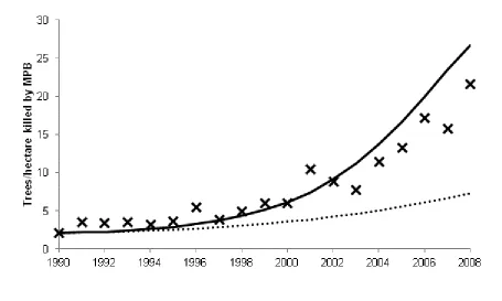
ponderosae Hopkins) plays an important role by removing older and less vigorous trees from the forest. Endemic MPB populations periodically surge creating a natural cycle and periods of considerable forest mortality. The region has experienced four to five significant outbreaks over the last century (Taylor and Carroll 2004) and is in the midst of an outbreak of unparalleled severity. Surveys conducted by the U.S.D.A. Forest Service (USDA FS) show that while the areal extent of the current outbreak is comparable to previous outbreaks, nearly three times the number of trees have been killed (see Figure 1). This forest mortality has resulted in billions of dollars in manufacturing losses (Abbott et al. 2008; Patriquin et al. 2007; Phillips et al. 2007) and numerous less obvious impacts.1

In order for endemic MPB populations to transition to a large-scale outbreak, two requirements must be satisfied. The first is a sustained period of favorable weather over several years. Winter temperature influences MPB populations through survival while summer

temperature and drought indirectly impact populations through MPB attack success which is required for reproduction (Carroll et al. 2004). Conventional wisdom appears to implicate

4

climate change and a recent sequence of abnormally warm years as the root cause of the increase in outbreak severity (Aukema et al. 2008; Carroll et al. 2004; Harrington et al. 2001; Logan and Powell 2001; Logan and Powell 2009)(see Figure 1). The implied argument is that the recent outbreak is abnormally severe because climate change allowed MPBs to successfully attack healthy trees that would have fought off attack in previous outbreaks. However, a second and more fundamental requirement for an outbreak is a sufficient stock of susceptible host trees. Large stocks of susceptible host trees combined with a homogenous forest structure increase the risk and severity of landscape-level MPB outbreaks (Safranyik and Carroll 2006). The vast majority of MPB habitat in the U.S. is public land administered by the USDA FS. As a result, public forest management has played an important role in the current outbreak by regulating the abundance of susceptible host trees.

5

evidence that preferences evolve according to individual and group interaction (see Durlauf and Young (2001), for a review). Changing preferences for ecosystem services of public forests thus provides an alternative economic explanation for the current outbreak. While climate change is undoubtedly a factor in the current outbreak, it is important to quantify the relative contribution of these two public forest management changes in an attempt to mitigate unintended climatic amplifications of MPB outbreaks.

This effort is complicated by diverse forest characteristics in MPB habitat ranging from low-elevation stands of ponderosa pine to high-elevation forests of lodgepole pine. The

6

The model demonstrates that changes in preferences and subsequent reductions in timber harvesting have exacerbated the MPB disturbance process in western forests. The result is robust when controlling for the influence of fire suppression, and occurs by increasing

susceptible hosts and amplifying the effect of climate change on MPB populations. While fire suppression may have played a larger role in certain forest types, it cannot fully explain the extent of the outbreak at a landscape scale without changes in preferences for ecosystem services.

II. BACKGROUND

Stretching from New Mexico to California and north into British Columbia, the majority of MPB habitat in the U.S. is public land administered by the Forest Service.3

This drop has been attributed to the mild recession in the early 1990s, softwood timber trade disputes between the U.S. and Canada starting in the mid-1980s, and federal timber sale restrictions in response to a number of high-profile environmental issues (Gorte 1994; Murray and Wear 1998; Wear and Murray 2004).

Management on these forests has evolved over time due to changes in society’s preferences for timber and non-timber ecosystem services provided from public lands. Following a major WWII expansion, USDA FS timber sales in MPB habitat leveled off after 1960 (Smith et al. 2009). Federal legislation such as the Multiple Use Sustained Yield Act of 1960, the Wilderness Act of 1964, and the National Forest Management Act of 1976 required forest outputs other than timber be given due consideration in the management of national forests. In 1990, USDA FS timber sales dropped precipitously in much of the western U.S.

4

7

price in the long-run (Berck 1979). The implication is that macroeconomic conditions and trade disputes may be capable of explaining the initial decline in harvests, but would be unable to explain the sustained reduction in timber sale offerings over the last two decades. Wear and Murray (2004) use an econometric model of the U.S. softwood lumber and timber markets to show that the decrease in public timber sale offerings cannot be explained by decreases in regional or national timber demand. They find that federal timber sale restrictions led to a shrinking market share for timber producers in the western U.S. Due to the restrictions and increasing public outcry for other non-timber benefits from public forests, the USDA FS began favoring ecosystem management over timber management as seen by the continued reduction in federal timber sales (Bengston 1994; Sedjo 1995).

III. THEORETICAL MODEL Ecological Model of Managed Forest

The ecological component of the model presents a dynamic predator-prey relationship between MPB and the forest with time set in annual increments to match the MPB lifecycle (Samman and Logan 2000).5 A representative forest model is presented which captures the general forest dynamics present in MPB habitat; specific forest types can be reflected by varying the model’s parameters. Following Heavilin and Powell (2008), the forest is homogeneous but divided into three size classes: seed base (𝑋), young trees (𝑌), and adult trees (𝐴). Young trees have a diameter at breast height (dbh) less than 8 inches. Although young trees have less

8

are also large enough to house egg galleries and act as an ample nutrient source. Each size class is measured in trees or seeds per hectare. The laws of motion for the beginning-of-period density in each size class are given by:

𝑋𝑡+1= (1− 𝛿𝑋)𝑋𝑡+𝑏𝑌𝑌𝑡+𝑏𝐴𝐴𝑡 [1]

𝑌𝑡+1 = (1− 𝛿𝑌− 𝜆𝑡)𝑌𝑡+𝛿𝑋𝑋𝑡 [2]

𝐴𝑡+1= (1�������������������− 𝑑 − 𝜋𝑡− 𝜆𝑡𝛾𝑡)𝐴𝑡+𝛿𝑌𝑌𝑡 𝐴_𝑡𝐻

− ℎ𝑡, [3]

where growth and mortality are assumed to occur prior to timber harvesting, differentiating the harvestable stock 𝐴_𝑡𝐻 from 𝐴_𝑡. Each year, a proportion (𝛿_𝑋 and 𝛿_𝑌) of the seed base and young trees mature to the successive size class. Contributions to the seed base are made by the young and adult size classes at rates 𝑏_𝑌 and 𝑏_𝐴. Only adult trees are considered viable for commercial harvest ht and susceptible to natural mortality (at constant rate𝑑) or MPB-induced mortality (at

time-varying rate𝜋_𝑡).

9 𝛾𝑡= _{1 +}𝑧(_𝑧𝑌𝑡_(𝑌+𝐴𝑡)

𝑡+𝐴𝑡), [4]

where 0 < 𝑧< 1 determines how much the abundance of young and adult trees contributes to fire severity. Increasing the fire return interval will leave more young and adult trees in the forest, which increases the severity of a fire. This captures the complex variations in fire regime between forest types. For example, ponderosa pine forests are characterized by frequent fires (I

< 30 years) of low severity while lodgepole pine forests are characterized by less frequent (I > 200 years) but more severe stand-replacing fires. To capture the less frequent but more severe fires resulting from fire suppression activities (Bradshaw and Lueck 2011; Holmes et al. 2008; Yoder and Blatner 2004), we assume the fire return interval is increasing over time (Gibson and Negron 2009) while holding the effects of harvesting on fuel load constant. There are additional means of fuel management (Amacher et al. 2005; Amacher et al. 2006) that reduce fire severity, but they are not considered here.

Successful MPB attacks cut off nutrient exchange between the roots and the tree, interupt water translocation, lower wood moisture content, and weaken defense mechanisms which eventually lead to tree death (Samman and Logan 2000). The probability a pine tree will die from MPB is determined by the interaction between the number of MPB attacking the tree and the level of tree resistance (Berryman et al. 1985). The probability of successful attack at the tree level translates into a known rate of MPB-induced mortality at the forest level. Following Heavilin and Powell (2008), we define the rate of MPB-induced mortality as

𝜋𝑡= 𝐵𝑡 2

10

where 𝐵_𝑡 is the number of MPB per hectare and 𝑎_𝑡 reflects the resistance of susceptible trees to MPB attack in year t. This parameter decreases as trees become drought-stressed or as the emergence of MPB – driven by temperature cues – become more synchronized in time, making the population of attacking beetles more effective in attacking new hosts. Equation [5] is

characteristic of the type III functional response in predator-prey interactions (Holling 1959) and captures threshold dynamics characteristic of MPB (Berryman et al. 1985). To be consistent with available USDA FS data, the severity of MPB damage is measured by the number of trees killed per hectare by MPB: 𝜋_𝑡𝐴_𝑡.

The relationship between MPB populations and the forest stock involves a one-year lag as adult MPBs typically emerge from the tree a year after initial infestation (Samman and Logan 2000). MPB density at time 𝑡is therefore a function of the density of successfully attacked trees at time 𝑡 −1 and the number of newly emerged beetles per successfully attacked tree,𝜑:

𝐵𝑡 =𝜑(𝜋𝑡−1𝐴𝑡−1)𝜈, [6]

where 𝜈 < 1 is a curvature parameter, modeling a proportional decrease in successful reproduction when large beetle populations begin to over-utilize available host resources. Together, equations [5] and [6] capture the recursive nature of the MPB population. Equations [1]-[3] and [5]-[6] have also been shown to successfully replicate data on MPB attack dynamics at a landscape level (Heavilin and Powell 2008).

Incorporating Climate Change: Thermal Response

11

temperature on MPB dynamics by allowing for a change in the overall reproductive success beetles have in any given year 𝜑 𝑎⁄ _𝑡 (Heavilin and Powell 2008).8

Since MPB development takes place in the phloem or inner bark of the tree, a thermal response model is used to connect measured phloem temperatures to the number of newly infested trees created by a single MPB-infested tree (Powell and Bentz 2009). The model is driven by hourly phloem temperatures for the year between the old and new attacks and

calculates a distribution of MPB emergence per day,𝑃(𝑡). The degree to which this distribution exceeds a critical threshold predicts the ratio of new-to-old infestations,𝑟_𝑡. Values of 𝑟_𝑡 grow or shrink depending on beetle lifecycle events, which are controlled by the phloem temperature. If the emergence distribution is narrow and steep (characteristic of higher average temperatures), the beetles are relatively effective in killing new hosts; broader emergence curves (lower mean temperatures) result in smaller values of𝑟_𝑡.

The thermal response model’s 𝑟_𝑡predictions can be correlated with the tree resistance parameter,𝑎_𝑡, in the bioeconomic model. We can then write 𝑎_𝑡 as a function of 𝑟_𝑡which links the results of the thermal response model with the ecological component of the bioeconomic model: 9

For a given adult tree stock, higher temperatures trigger larger values of 𝑟_𝑡 thereby lowering host tree resistance.

𝑎𝑡 =𝜑 �0.5_𝑟𝐴𝑡 𝑡 �

𝜈

. [7]

Ecosystem Service Production in MPB Habitat

Society in the model is made up of many identical households, which receive

12

derived from public forests. Ecosystem services are comprised of timber products ℎ_𝑡and non-timber services such as amenity values, wildlife habitat, and biodiversity. Non-non-timber ecosystem services depend on the quality of the forest resource (Englin et al. 2000), proxied by the stock of living adult trees𝐴_𝑡𝐻.10

where 𝛼_𝑡 is the non-timber preference parameter which captures the relative weight households place on non-timber ecosystem services in relation to timber ecosystem services. We normalize the non-timber preference parameter to the unit interval 0≤ 𝛼_𝑡≤ 1.

For tractability, period 𝑡 utility of the representative household is given by:

𝑈(𝑄𝑡,ℎ𝑡,𝐴𝑡𝐻;𝛼𝑡) = 𝑙𝑛(𝑄𝑡) + (1− 𝛼𝑡)𝑙𝑛(ℎ𝑡) +𝛼𝑡𝑙𝑛(𝐴𝑡𝐻), [8]

11

Each year the representative household inelastically supplies 𝐿= 𝐿𝑄_𝑡 +𝐿_𝑡𝐴 units of labor, which are allocated between the production of the composite commodity (𝐿𝑄_𝑡) and the production of timber products (𝐿𝐴_𝑡). Production of Qt is directly proportional to labor inputs: 𝑄_𝑡= 𝐿𝑄_𝑡. Harvesting adult timber requires labor and depends on the harvestable stock according to harvest function:

ℎ𝑡 =𝜌𝐿𝐴𝑡𝐴𝑡𝐻, [9]

It is through changes in 𝛼𝑡 that the model can track changes in social attitudes towards ecosystem services over time.

13

harvest levels are supplied by USDA FS data, ignoring salvage harvests will not change the decline in harvest levels or harvesting’s contribution to the MPB outbreak.

Optimal forest management seeks an appropriate balance between timber and non-timber ecosystem services given societal preferences. However, there may be political and judicial factors that cause changes in forest management to lag changes in preferences. Specifically, a social planner chooses a harvest program to solve the following problem:13

where 0 ≤ β≤ 1 is the annual discount factor and s≥ 0 allows for any lag between changes in preferences and timber harvesting. The problem in [10] is solved subject to the ecological equations of motion [1] – [6], initial conditions for stocks, and the constraints:

𝑄𝑡+_𝜌𝐴ℎ𝑡 𝑡

𝐻 =𝐿 [10𝑎]

ℎ𝑡 > 0. [10𝑏]

max

{ℎ𝑡}𝑡=1∞ � 𝛽

𝑡−1_𝑈(𝑄

𝑡,ℎ𝑡,𝐴𝑡𝐻;𝛼𝑡−𝑠),

∞

𝑡=1 [10]

The solution to [10] is found through a series of substitutions that incorporate all

applicable dynamics, changing the choice variable from harvest to stock of adult trees (Azariadis 1993). Normalizing labor supply to one, the first-order condition requires harvesting to proceed until the discounted future marginal benefits and costs are equal.14

The discounted future benefit of harvesting an additional tree is �1− 𝛼_ℎ 𝑡−𝑠

𝑡 �+𝛽 �Ψ𝑡+1

𝜕𝐴𝑡+1𝐻

𝜕𝛾𝑡+1

𝜕𝛾𝑡+1

𝜕𝐴𝑡+1

𝜕𝐴𝑡+1

𝜕ℎ𝑡 �+

� 𝛽𝑘_�Ψ

𝑡+𝑘𝜕𝐴𝑡+𝑘 𝐻 𝜕𝜋𝑡+𝑘 𝜕𝜋𝑡+𝑘 𝜕𝐵𝑡+𝑘 𝜕𝐵𝑡+𝑘 𝜕𝐴𝑡+1 𝜕𝐴𝑡+1

𝜕ℎ𝑡 � ∞

𝑘=2

+� 𝛽𝑘_Ψ

𝑡+𝑘∆𝑡+𝑘𝑠𝑒𝑒𝑑→𝑓𝑖𝑟𝑒 ∞

𝑘=3

, [11]

14 Ψ𝑡= 1− 𝛼_ℎ 𝑡−𝑠

𝑡 −

𝐴𝑡𝐻− ℎ𝑡

𝑄𝑡𝜌(𝐴𝑡𝐻)2+

𝛼𝑡−𝑠

𝐴_𝑡𝐻 [12]

is the marginal net benefit of an adult tree at time 𝑡. Equation [11] contains both direct and indirect benefits of harvesting. The first term in [11] represents the immediate benefit of timber harvesting. Harvesting in period 𝑡 also indirectly lowers the severity of fires by reducing the adult stock in 𝑡+ 1 (second term) and reduces MPB risk by lowering the MPB stock in 𝑡+ 2. Harvesting also recursively lowers MPB risk in all future periods (third term). The last term is the present value at t + 3 of lower fire damage in all future periods working through the seed effect. Due to the relatively slow growth of a forest, this effect is negligible.

The discounted future cost of harvesting an additional tree is 1

𝑄𝑡𝜌𝐴𝐻𝑡 + 𝛽{Ψ𝑡+1(1− 𝑑 − 𝜋𝑡+1− 𝜆𝑡+1𝛾𝑡+1)} +� 𝛽 𝑘_Ψ

𝑡+𝑘∆𝑡+𝑘𝑠𝑒𝑒𝑑 ∞

𝑘=3

. [13]

The first term represents the labor cost of harvesting in terms of reduced production of the composite commodity. Harvesting a tree in period 𝑡 means it is not available to provide utility for timber and non-timber benefits in period𝑡+ 1. The opportunity cost in 𝑡+ 1 of harvesting in period 𝑡(second term) is lower because the tree may be killed by fire or MPB (at time-varying rates 𝜆_𝑡+1𝛾_𝑡+1 and𝜋_𝑡+1) or natural causes (at rate𝑑) before next period’s harvesting decision. The last term is negligible and represents the present value at 𝑡+ 3 of the reduction in the future seed base caused by harvesting in period𝑡.

The optimal harvest condition found by equating [11] and [13] provides a rule to

determine optimal harvest management for a given set of model parameters and preferences. If observed annual USDA FS harvest data are assumed to optimally respond to changes in

15

non-timber ecosystem services,𝛼_𝑡−𝑠. The derived value of 𝛼_𝑡−𝑠 is consistent with stocks that are determined by the equations of motion given observed harvests.

IV. DYNAMIC CALIBRATION

To derive the values for 𝛼_𝑡−𝑠 implied from observed data, the model is simulated as if

observed harvests were optimal while controlling for both the effects of fire suppression15 and the echo effects of previous large-scale disturbances.16 Figure 1 shows observed values for public forest timber sales, temperature and hectares burned for the years 1960 through 2008, and hectares of MPB infestations and trees killed by MPB from 1977 through 2008. Each variable displays a relatively constant or declining trend prior to 1990. After 1990, timber harvests plummet while average temperatures, hectares burned, hectares of MPB infestations, and trees killed by MPB all rise. The sample period contains all the relevant drivers needed to determine the contributions of climate change, fire suppression, and timber harvests in the current MPB epidemic.

Model Parameters

Table 1 presents a set of economic and ecological parameters selected to obtain a realistic initial condition in 1960 consistent with the observed harvest level. This condition is

characterized by 8,397 MPB, 57,000 seeds, and 499 adult trees per hectare. The sensitivity of model results to selected parameter values is investigated in the appendix. The first step in the calibration process determines the scale parameter 𝜌 measuring the efficiency of adult

16

harvesting effort. This parameter is scaled to 0.03255 to provide an initial condition where society equally values timber and non-timber ecosystem services: 𝛼_1960−𝑠= 0.5.17

The discount rate is set to 4% (implying an annual discount factor of 𝛽 = 0.96) in accordance with USDA FS practice (Row et al. 1981). Natural mortality (d) is set to 1.5% (Runkle 1985). The parameters dictating seed production (𝑏_𝑉,𝑏_𝐴), germination (𝛿_𝑋), and maturation (𝛿_𝑌) in Table 1 produce a comparable and defensible initial condition typical of USDA FS land in the western U.S. (Koch 1996).

18

Fire-specific parameters 𝐼 and 𝑧 are based on fire regimes found in MPB habitat. Fire regimes are generally classified based on fire return interval 𝐼 (frequency) and the percent replacement of overstory trees 𝛾_𝑡(severity) (Hann and Bunnell 2001). The fire regime in MPB habitat has historically ranged from frequent fires of low severity (𝐼< 30 and 𝛾_𝑡< 25%) to less frequent stand-replacing fires (𝐼 > 200 and 𝛾_𝑡> 75%) (Romme et al. 2006). We assume the fire return interval is initially 100 years and 𝑧 is selected to provide an initial fire severity of 50%: 𝑧= 0.00054. To illustrate the effect of fire suppression on fire regimes, we increase the fire return interval by 6 months for every year from 1960 to 2008. This corresponds to a 50% departure over the nearly 100 years fire suppression has taken place on public lands.

These forest-specific parameters allow the forest to re-establish within 80 to 140 years following a stand-replacing disturbance (Lotan and Critchfield 1990).

19

MPB-specific parameters𝑎_𝑡,𝜑, and ν depend on site conditions, tree species, climate, and geography among other things. Proportional changes in 𝑎_𝑡and 𝜑 have little impact on the

17

model. The key value is the ratio of beetle reproductive success to tree resistance: 𝜑/𝑎_𝑡. Using aerial survey data, Heavilin and Powell (2008) estimate this ratio to be approximately 0.071 in 1990. Previous studies provide multiple measures of 𝜑 by counting the number of beetles emerging from an infested tree (e.g., Bentz 2006). These studies generally place 𝜑 between 4,000 and 5,000 beetles per infested tree. This suggests 𝑎₁₉₉₀ is approximately 157,653 beetles per hectare, assuming 𝜑 = 4,500 beetles per infested tree. In the absence of data prior to 1990 and as discernable changes in temperature in the western U.S have been relatively recent (see Figure 1), we assume this level of tree resistance was constant prior to 1990. Finally Berryman et al. (1985) report a decreasing relationship between MPB offspring and the number of MPB attacks per square meter of tree surface area. This indicates decreasing reproductive returns from increases in adult-tree mortality and implies a degree of curvature in [6]. In the absence of any additional quantitative results to guide us, we set ν = 0.5.

Measuring Implied Preferences for Non-timber Ecosystem Services

18

Necessary data to measure implied preferences include annual harvest of live (green) trees from National Forests in the geographic range of MPB (USDA FS regions 1 through 6). While annual USDA FS harvest data are publically available from Cut and Sold Reports at a regional level, these Reports do not distinguish between harvests of live and dead trees. Periodic Timber Sale Accomplishment Reports (PTSAR) do distinguish annual live timber sales on USDA FS land and were used as a proxy forℎ_𝑡.21 These board foot volume measures of total harvests must be converted to trees per hectare. Using historic data from the USDA FS Land Areas Reports (LAR) from 1997 through 2008, we calculate that regions 1 through 6 consistently make up 75% of total USDA FS area. This hectare measure is used to calculate average board feet per hectare of live timber sold within the geographic range of MPB. The board feet measure is then converted to trees per hectare assuming 25 board feet per tree which is consistent with an 80-year old stand of lodgepole pine.22

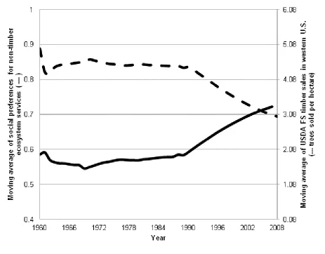
Model projections show that the decrease in adult timber harvesting after 1990 follows an increase in preferences for non-timber ecosystem services (moving averages shown in Figure 2). This corresponds to Wear and Murray’s findings (Wear and Murray 2004). However, forest management alone is not capable of replicating the MPB-induced mortality witnessed between 1990 and 2008. The dotted line in Figure 3 shows MPB-induced tree mortality controlling for the effects of fire suppression and changes in timber harvesting. In addition to the changes in forest management, this period has also seen an increase in mean annual temperature throughout the western United States (Figure 1). Temperature increases raise MPB attack success by synchronizing adult beetle emergence and increasing survival. In addition to underestimating MPB-induced mortality, ignoring the influence of climate also fails to capture the full effect of

19

the shift in preferences. Since increasing temperatures cause trees to be more susceptible to MPB attack, society’s desire to leave more trees in the forest also amplifies the effects of climate change on MPB populations. For these reasons, it is essential to accurately measure the effect of climate change in our bioeconomic model.

Measuring the Effect of Climate Change

To parameterize the thermal response model, hourly phloem temperatures are needed for the year between the old and new attacks. A continuous south-side phloem temperature record exists from July 19, 1992 through August 18, 2003 for a MPB outbreak in the Stanley Valley of central Idaho. The phloem temperature record is used to project temperatures for the years 1990-2050 assuming a 0.0443 Co/year increasing trend in annual mean temperatures.

Using nonlinear rate curves and fitted variances for all eight developmental phases

through which a MPB must pass between host attack and emergence of brood to attack new hosts the following year, a distribution of MPB emergence per day, 𝑃, is calculated. The degree to which this distribution exceeds a critical threshold predicts the ratio of new-to-old infestations, 𝑟𝑡:

𝑟𝑡= � max(8.10𝑃(𝜏)−0.181,0)𝑑𝜏 245

152 . [14]

where 152 and 245 are the Julian Day (JD) measures for June 1 and August 30 in the year of beetle emergence.23 The values 8.10 and 0.181 are maximum likelihood estimates for reduced form biological parameters using phloem temperatures measured on the south (warm) side of hosts in the Stanley Valley.24

Using 𝜑= 4500 MPB per tree, ν = 0.5, and a reasonable estimate of initial host density

20 𝑎𝑡 = 63640

�𝑟𝑡 . [15]

The thermal response model was simulated for each year using the temperature projections and tree resistance trajectories outlined above.

To avoid projecting temperature anomalies in the Stanley Valley to the rest of the western U.S., we use the results of the thermal response model to calculate trends in tree resistance. A logarithmic regression was used to estimate constant exponential rates of decrease in 𝑎_𝑡 from these data, generating rates ranging from -0.29% to -1.1% per year depending on the base year. Combined with historic harvest levels and an increasing fire return interval, we find that a decrease in 𝑎_𝑡 of 0.65% per year is capable of replicating the historic levels of MPB-induced mortality witnessed between 1990 and 2008 (solid lines in Figure 3). These results incorporate historic changes in preferences for ecosystem services, fire suppression, and the effects of climate change.

V. ISOLATING THE EFFECT OF FOREST MANAGEMENT

To illustrate the implications of the model we construct a benchmark that replicates historic MPB-induced mortality by accounting for changes in preferences for ecosystem services, fire behavior, and climate. The shift towards non-timber ecosystem services creates a direct effect on MPB-induced mortality by leaving more susceptible trees in the forest. Fire

21

trees left in the forest due to changing preferences and fire suppression are now more vulnerable to MPB attack as a result of climate change.

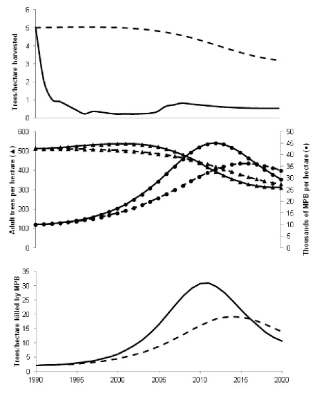
To capture the peak of the current outbreak we simulate past 2008. Preferences are assumed to remain at the 2007 level while changes in fire behavior and climate continue to impact forest and MPB dynamics through 2020, at which time the outbreak will have largely run its course. This allows optimal harvest levels to be calculated from 2009 to 2020. Combining these simulated harvest levels with the observed harvest levels allows us to calculate MPB and forest dynamics over the entire outbreak as shown in the solid lines in Figure 4.

The period 1990 to 2008 is characterized by a sharp decrease in harvest levels along with a brief increase in harvest levels at the end of the period. Projecting the model into the future, optimal management calls for a gradual decrease in harvest levels from 2009 to 2020 as the stock of trees is reduced by MPB. In this benchmark model, the increasing importance of non-timber ecosystem services and the general decline in harvests combine with fire suppression and a changing climate to induce cycles in the MPB stock due to “echo effects” inherent in the

ecological model. Such cycles are a natural MPB phenomenon causing an outbreak that peaks in 2011 at approximately 30.9 trees per hectare killed.

22

outbreak that peaks in 2012 at approximately 29.2 trees per hectare killed. In the scenario of invariant preferences, the social planner responds to climate driven increases in MPB-induced mortality by gradually reducing harvest levels as opposed to the drastic decline in harvests when preferences shift (Figure 4A). This counterfactual scenario sees more trees harvested, fewer trees available for MPB to attack, and a less severe increase in MPB populations (Figure 4B). The result is a delayed and less severe MPB outbreak that peaks in 2014 at 19.3 trees per hectare killed (Figure 4C).

Consistent with previous research (Wear and Murray 2004), results indicate that the decrease in adult timber harvesting after 1990 follows an increase in preferences for non-timber ecosystem services. The bioeconomic model takes this result one step further. Given the effects of fire suppression, the decrease in timber harvesting left more susceptible trees standing in the forest, which directly increased MPB populations even in the absence of climate change. These additional trees have also become more susceptible to MPB attack due to the impact of climate change. The result has been a shift in the ecological regime from a primarily

climate-independent disturbance processes (timber harvesting) to a climate-dependent one (MPB outbreaks).

VI. CONCLUSIONS

23

outbreak. A larger portion is explained by the sharp decrease in timber harvesting after 1990, which is consistent with a shift in preferences toward valuing the forest for non-timber

ecosystem services such as amenity value, wildlife habitat and biodiversity.26

While our results present a general overview, it is important to note that fire suppression and changes in preferences for ecosystem services may have played more or less of a role in the current MPB outbreak in specific forest types. For example, fire suppression is expected to have a minimal impact in lodgepole pine and subalpine forests whose historic fire return interval is greater than 100 years (Romme et al. 2006). However, in the ponderosa pine forests of Arizona, New Mexico, and southern Colorado, the fire return interval is historically much shorter,

implying a greater role for fire suppression in this forest type (Romme et al. 2006). If the

objective is to apply our results to a specific forest type, forest estate models may be a preferable alternative to the more general model of forest dynamics presented herein.

This shift toward non-timber ecosystem services and the subsequent reduction in harvesting led to more

susceptible trees in the forest and an increase in MPB-induced mortality that temporally corresponds to the ongoing outbreak in the western United States. The increase in susceptible trees also exacerbates the effects of climate change, which amplified MPB outbreaks further. While simulations suggest that climate change is a primary driver of the MPB epidemic, the shift in preferences for ecosystem services indirectly expedited the MPB outbreak and substantially increased tree mortality. This result implies that the current unprecedented MPB outbreak is, to a large extent, an artifact of the fundamental change in public forest management that took place nearly two decades ago.

24

and the initiation of fire suppression activities, timber harvesting became the dominant

disturbance regime. The shift toward non-timber ecosystem services eliminated harvesting as a dominant disturbance. In its absence, MPB-induced mortality appears to be claiming that role, implying larger MPB outbreaks even if climatic factors were held constant. However, as a growing body of evidence indicates, the MPB’s role as a natural disturbance agent may be fundamentally altered by climate change, leading to even more severe outbreaks in the future. The shift in social attitudes for ecosystem services therefore not only helped create the current outbreak by leaving more trees in the forest but also exacerbated the effects of climate change by shifting from a relatively climate-independent disturbance regime (timber harvesting) to a

climate-dependent one (MPB outbreaks).

25 Appendix

Derivation of Euler Equation – Substitution Method

A social planner chooses harvesting levels to maximize:

� 𝛽𝑡−1_{{𝑙𝑛(𝑄}

𝑡) + (1− 𝛼𝑡−𝑠)𝑙𝑛(ℎ𝑡) +𝛼𝑡−𝑠𝑙𝑛(𝐴𝐻𝑡)} ∞

𝑡=1 [A. 1]

subject to [1]-[6] and [10a] from the main body of the paper. The need to link harvests with the preference parameter 𝛼_𝑡−𝑠 requires a single optimality condition. As all constraints are given by equalities, a method of substitution is followed (Azariadis 1993). All the biological and

economic constraints are substituted into [A.1], changing the choice variable from ℎ_𝑡 to𝐴_𝑡+1. Later in the appendix we show that this method is equivalent to the method of Lagrangian multipliers.

First, labor endowments are normalized to one such that𝐿𝑄_𝑡 = 1− 𝐿_𝑡𝐴. Noting that 𝐴𝑡𝐻 =𝐴𝑡+1+ℎ𝑡 and substituting [10a], we can rewrite [A.1] as:

� 𝛽𝑡−1_{�𝑙𝑛 �1−} ℎ𝑡

𝜌(𝐴𝑡+1+ℎ𝑡)�+ (1− 𝛼𝑡−𝑠)𝑙𝑛(ℎ𝑡) +𝛼𝑡−𝑠𝑙𝑛(𝐴𝑡+1+ℎ𝑡)� ∞

𝑡=1 . [A. 2]

To account for the ecological components, we start by substituting [4] and [5] into [3] to get:

ℎ𝑡= �1− 𝑑 − 𝐵𝑡 2

𝐵𝑡2+𝑎2− 𝜆𝑡

𝑧(𝑌𝑡+𝐴𝑡)

1 +𝑧(𝑌𝑡+𝐴𝑡)� 𝐴𝑡+𝛿𝑌𝑌𝑡− 𝐴𝑡+1. [A. 3]

26 ℎ𝑡 =�1− 𝑑 − (𝜑(𝜋𝑡−1𝐴𝑡−1)

𝜈₎2

(𝜑(𝜋𝑡−1𝐴𝑡−1)𝜈)2+𝑎2− 𝜆𝑡

𝑧((1− 𝛿𝑌− 𝜆𝑡−1)𝑌𝑡−1+𝛿𝑋𝑋𝑡−1+𝐴𝑡)

1 +𝑧((1− 𝛿𝑌− 𝜆𝑡−1)𝑌𝑡−1+𝛿𝑋𝑋𝑡−1+𝐴𝑡)� 𝐴𝑡

+𝛿𝑌(1− 𝛿𝑌− 𝜆𝑡−1)𝑌𝑡−1+𝛿𝑌𝛿𝑋𝑋𝑡−1− 𝐴𝑡+1. [A. 4]

Finally, substituting [1] into [A.4] yields:

ℎ𝑡 =

⎝ ⎜

⎛ 1− 𝑑 −

(𝜑(𝜋𝑡−1𝐴𝑡−1)𝜈)2

(𝜑(𝜋𝑡−1𝐴𝑡−1)𝜈)2+𝑎2

−𝜆𝑡_{1 +}𝑧((1_𝑧((1− 𝛿_{− 𝛿}𝑌− 𝜆𝑡−1)𝑌𝑡−1+𝛿𝑋(1− 𝛿𝑋)𝑋𝑡−2+𝛿𝑋𝑏𝑌𝑌𝑡−2+𝛿𝑋𝑏𝐴𝐴𝑡−2+𝐴𝑡) 𝑌− 𝜆𝑡−1)𝑌𝑡−1+𝛿𝑋(1− 𝛿𝑋)𝑋𝑡−2+𝛿𝑋𝑏𝑌𝑌𝑡−2+𝛿𝑋𝑏𝐴𝐴𝑡−2+𝐴𝑡)_⎠

⎟ ⎞

𝐴𝑡

+𝛿𝑌(1− 𝛿𝑌− 𝜆𝑡−1)𝑌𝑡−1+𝛿𝑌𝛿𝑋(1− 𝛿𝑋)𝑋𝑡−2+𝛿𝑌𝛿𝑋𝑏𝑌𝑌𝑡−2+𝛿𝑌𝛿𝑋𝑏𝐴𝐴𝑡−2− 𝐴𝑡+1 [A. 5]

Due to the recursive nature of the MPB dynamics and the forest stocks, one must continually substitute π, B, X and Y into [A.5] to fully account for the shadow value of B, X,and

Y. The resulting expression can then be substituted into [A.2] to fully account for equations [1]-[6] and [10a]. This substitution procedure also changes the choice variables from harvests to the stock of adult trees. A similar solution procedure is described in Azariadis (1993) and was used in previous research to study the effect of cattle cull rates on the age structure of a cattle stock (Aadland 2004). Following the series of substitutions outlined above and taking derivatives with respect to 𝐴_𝑡+1 yields our first-order condition for welfare maximizing levels of harvest:

1− 𝛼𝑡−𝑠

ℎ𝑡 −

1

𝑄𝑡𝜌𝐴𝑡𝐻+𝛽 �Ψ𝑡+1

𝜕𝐴𝑡+1𝐻

𝜕𝛾𝑡+1

𝜕𝛾𝑡+1

𝜕𝐴𝑡+1

𝜕𝐴𝑡+1

𝜕ℎ𝑡 �+� 𝛽 𝑘_�Ψ

𝑡+𝑘𝜕𝐴𝑡+𝑘 𝐻 𝜕𝜋𝑡+𝑘 𝜕𝜋𝑡+𝑘 𝜕𝐵𝑡+𝑘 𝜕𝐵𝑡+𝑘 𝜕𝐴𝑡+1 𝜕𝐴𝑡+1

𝜕ℎ𝑡 � ∞

27 +� 𝛽𝑘_�Ψ

𝑡+𝑘∆𝑡+𝑘𝑠𝑒𝑒𝑑→𝑓𝑖𝑟𝑒� ∞

𝑘=3

=𝛽{Ψ𝑡+1(1− 𝑑 − 𝜋𝑡+1− 𝜆𝑡+1𝛾𝑡+1)} +� 𝛽𝑘�Ψ𝑡+𝑘∆𝑡+𝑘𝑠𝑒𝑒𝑑� ∞

𝑘=3

[A. 6]

where

∆_𝑡+𝑘𝑠𝑒𝑒𝑑→𝑓𝑖𝑟𝑒=𝜕𝐴𝑡+𝑘𝐻

𝜕𝛾𝑡+𝑘 𝜕𝛾𝑡+𝑘 𝜕𝑌𝑡+𝑘 𝜕𝑌𝑡+𝑘 𝜕𝑋𝑡+𝑘−1 𝜕𝑋𝑡+𝑘−1 𝜕𝐴𝑡+1 𝜕𝐴𝑡+1

𝜕ℎ𝑡 [A.7] ∆𝑡+𝑘𝑠𝑒𝑒𝑑= 𝜕𝐴𝑡+𝑘

𝐻 𝜕𝑌𝑡+𝑘 𝜕𝑌𝑡+𝑘 𝜕𝑋𝑡+𝑘−1 𝜕𝑋𝑡+𝑘−1 𝜕𝐴𝑡+1 𝜕𝐴𝑡+1

𝜕ℎ𝑡 [A.8]

Equations [A.7] and [A.8] indicate the complexity of the “seed effect” terms succinctly presented as ∆_𝑡+𝑘𝑠𝑒𝑒𝑑→𝑓𝑖𝑟𝑒 and ∆_𝑡+𝑘𝑠𝑒𝑒𝑑 in the text.

Alternative Dynamic Optimization – Method of Lagrangian Multipliers

An alternative solution method is to use the method of Lagrangian multipliers. The present value Lagrangian expression for the problem is:

𝐿=� 𝛽𝑡_{�𝑙𝑛 �𝐿 −} ℎ𝑡

𝜌𝐴𝐻_𝑡�+ (1− 𝛼𝑡)𝑙𝑛(ℎ𝑡) +𝛼𝑡𝑙𝑛(𝐴𝑡𝐻) +𝜆𝑡𝐴𝐻[(1− 𝑑 − 𝜋𝑡− 𝜆𝑡𝛾𝑡)𝐴𝑡+𝛿𝑌𝑌𝑡− 𝐴𝑡𝐻] ∞

𝑡=0

+𝛽𝜆𝑡+1𝐴 _[𝐴𝑡𝐻_{− ℎ𝑡− 𝐴𝑡+1] +𝛽𝜆𝑡+1}𝑋 _{[(1− 𝛿𝑋)𝑋𝑡+𝑏𝑌𝑌}

𝑡+𝑏𝐴𝐴𝑡− 𝑋𝑡+1]

+𝛽𝜆𝑌𝑡+1[(1− 𝛿𝑌− 𝜆𝑡)𝑌𝑡+𝛿𝑋𝑋𝑡− 𝑌𝑡+1]+𝛽𝜆𝐵𝑡+1[𝜑(𝜋𝑡𝐴𝑡)𝜈− 𝐵𝑡+1]�, [A. 9]

28

𝑡+ 1. They provide a signal to the decision maker in period 𝑡 of the opportunity costs or gains of harvests.

First-order conditions with respect to the control and state variables (ℎ_𝑡, 𝐴_𝑡𝐻, 𝐴_𝑡,𝑋_𝑡, 𝑌_𝑡 and 𝐵_𝑡) are:

𝜕𝐿 𝜕ℎ𝑡 =

1− 𝛼𝑡

ℎ𝑡 −

1 𝜌𝐴_𝑡𝐻_{�𝐿 − ℎ}𝑡

𝜌𝐴𝑡𝐻�

− 𝛽𝜆𝑡+1𝐴 = 0 [A. 10]

𝜕𝐿 𝜕𝐴𝑡𝐻 =

𝛼𝑡

𝐴𝑡𝐻+

ℎ𝑡

𝜌(𝐴_𝑡𝐻₎2_{�𝐿 − ℎ}𝑡

𝜌𝐴𝑡𝐻�

+𝛽𝜆𝑡+1𝐴 − 𝜆𝑡𝐴𝐻 = 0 [A. 11]

_𝜕𝐴𝜕𝐿

𝑡 =�1− 𝑑 − 𝜋𝑡− 𝜆𝑡𝛾𝑡−

𝜆𝑡𝛾𝑡𝐴𝑡

𝑌𝑡+𝐴𝑡(1− 𝛾𝑡)� 𝜆𝑡 𝐴𝐻₊

𝑏𝐴𝛽𝜆𝑡+1𝑋 +𝜈𝐵𝑡 2_𝜑(𝜋

𝑡𝐴𝑡)𝜈−1

𝐵𝑡2+𝑎𝑡2 𝛽𝜆𝑡+1

𝐵 _{− 𝜆}

𝑡

𝐴 _{= 0 [A. 12]}

𝜕𝐿

𝜕𝑋𝑡= (1− 𝛿𝑋)𝛽𝜆𝑡+1

𝑋 _+𝛿

𝑋𝛽𝜆𝑌𝑡+1− 𝜆𝑡𝑋 = 0 [A. 13]

𝜕𝐿

𝜕𝑌𝑡= �𝛿𝑌−

𝜆𝑡𝛾𝑡𝐴𝑡

𝑌𝑡+𝐴𝑡(1− 𝛾𝑡)� 𝜆𝑡 𝐴𝐻_+𝑏

𝑌𝛽𝜆𝑡+1𝑋 + (1− 𝛿𝑌− 𝜆𝑡)𝛽𝜆𝑌𝑡+1− 𝜆𝑡𝑌= 0 [A. 14]

𝜕𝐿 𝜕𝐵𝑡 =− �

2𝐴𝑡𝐵𝑡

𝐵𝑡2+𝑎𝑡2(1− 𝜋𝑡)� 𝜆𝑡

𝐴𝐻_{+�𝜈𝜑(𝜋}

𝑡𝐴𝑡)𝜈−1_𝐵2𝐴𝑡𝐵𝑡

𝑡2+𝑎𝑡2(1− 𝜋𝑡)� 𝛽𝜆𝑡+1

𝐵 _{− 𝜆}

𝑡

𝐵 _{= 0. [A. 15]}

First-order conditions with respect to the co-state variables (𝜆_𝑡+1𝑖 ) are:

𝜕𝐿

𝜕𝜆𝑡𝐴𝐻 = (1− 𝑑 − 𝜋𝑡− 𝜆𝑡𝛾𝑡)𝐴𝑡+𝛿𝑌𝑌𝑡− 𝐴𝑡

𝐻_{= 0 [A. 16]}

𝜕𝐿

𝜕𝜆𝑡+1𝐴 =𝐴𝑡 𝐻_{− ℎ}

29 𝜕𝐿

𝜕𝜆_𝑡+1𝑋 = (1− 𝛿𝑋)𝑋𝑡+𝑏𝑌𝑌𝑡+𝑏𝐴𝐴𝑡− 𝑋𝑡+1 = 0 [A. 18]

𝜕𝐿

𝜕𝜆_𝑡+1𝑌 = (1− 𝛿𝑌− 𝜆𝑡)𝑌𝑡+𝛿𝑋𝑋𝑡− 𝑌𝑡+1 = 0 [A. 19]

𝜕𝐿

𝜕𝜆_𝑡+1𝐵 =𝜑(𝜋𝑡𝐴𝑡)𝜈 − 𝐵𝑡+1= 0. [A. 20]

Optimality condition [A.10] requires harvesting to be expanded until the net marginal benefits of harvesting in the current period just equals the marginal cost of harvesting (in terms of forgone use of labor to produce Q):

1− 𝛼𝑡

ℎ𝑡 − 𝛽𝜆𝑡+1

𝐴 ₌ 1

𝜌𝐴_𝑡𝐻_{�𝐿 − ℎ}𝑡

𝜌𝐴𝑡𝐻�

[A. 10a]

Net marginal benefits subtract the opportunity cost of harvests (𝛽𝜆_𝑡+1𝐴 ), which is the discounted value of an additional adult tree in period𝑡+ 1.

For the harvestable stock of adult trees, equation [A.11] can be rewritten as:

𝜆𝑡𝐴𝐻 = _𝐴𝛼𝑡 𝑡

𝐻+ ℎ𝑡

𝜌(𝐴𝑡𝐻)2�𝐿 − ℎ_𝜌𝐴𝑡 𝑡 𝐻�

+𝛽𝜆𝑡+1𝐴 [A. 11a]

30

the tree standing. The third term is the 𝑡+ 1 marginal value of an adult tree left standing in period𝑡.

The value of adult trees throughout the ecosystem is differentiated from that of the harvestable stock following [A.12]:

𝜆𝑡𝐴 = �1− 𝑑 − 𝜋𝑡− 𝜆𝑡𝛾𝑡−_𝑌𝜆𝑡𝛾𝑡𝐴𝑡

𝑡+𝐴𝑡(1− 𝛾𝑡)� 𝜆𝑡 𝐴𝐻_+𝑏

𝐴𝛽𝜆𝑡+1𝑋 +𝜈𝐵𝑡 2_𝜑(𝜋

𝑡𝐴𝑡)𝜈−1

𝐵𝑡2+𝑎𝑡2 𝛽𝜆𝑡+1

𝐵 _{. [A. 12a]}

The value of an additional adult comes from three additive sources. The first follows from its availability for harvests where this magnitude is diminished by natural mortality (𝑑), the probability of a successful beetle attack (𝜋_𝑡) and the fire risk – not only in total (𝜆_𝑡𝛾_𝑡) but the marginal increase in fire risk from an additional adult (𝜆𝑡𝛾𝑡𝐴𝑡

𝑌𝑡+𝐴𝑡(1− 𝛾𝑡)). The second is through the contributions of adults in period 𝑡to the seed base in period𝑡+ 1. The third is a reduction in the value of an additional adult tree that follows from an increase in beetles.

Equation [A.13] provides the value of an additional unit of the seed base under optimal harvests:

𝜆𝑡𝑋= (1− 𝛿𝑋)𝛽𝜆𝑡+1𝑋 +𝛿𝑋𝛽𝜆𝑌𝑡+1. [A. 13a]

The seed base in 𝑡 has value through its (net) own growth plus its contribution to the young tree class.

The value of an additional young tree from [A.14] is:

𝜆𝑌𝑡 = �𝛿𝑌−_𝑌𝜆𝑡𝛾𝑡𝐴𝑡

𝑡+𝐴𝑡(1− 𝛾𝑡)� 𝜆𝑡 𝐴𝐻_+𝑏

31

The first term captures the value of a young tree that transitions to being a harvestable adult and the contribution to the marginal fire risk. A young tree also has value as it contributes to the seed base (second term) and contributes to its own growth (third term) net of its contributions to adults and fire mortality.

The final value the optimal program uncovers is that of the beetle stock from [A.15]:

𝜆𝑡𝐵= − �_𝐵2𝐴𝑡𝐵𝑡

𝑡2+𝑎𝑡2(1− 𝜋𝑡)� 𝜆𝑡

𝐴𝐻_{+�𝜈𝜑(𝜋}

𝑡𝐴𝑡)𝜈−1_𝐵2𝐴𝑡𝐵𝑡

𝑡2+𝑎𝑡2(1− 𝜋𝑡)� 𝛽𝜆𝑡+1

𝐵 _{. [A. 15a]}

An additional beetle in period 𝑡causes a loss of harvestable adult trees (first term) and a loss in value due to the increase in the 𝑡+ 1 stock of beetles (second term).

Equations [A.16] through [A.20] require the ecosystem dynamics to follow the given laws of motion. The equations of optimality must be simultaneously solved over all time periods given the initial conditions on the state variables and the transversality conditions (Azariadis 1993, p.211):

lim𝑡→∞𝛽𝑡𝜆𝑡𝑊𝑊𝑡 = 0

32

Reconciling the Substitution and Lagrangian Multiplier Methods

In contrast to the more traditional Lagrangian multiplier method, we chose to present the results from the substitution procedure as described in the first section of this Appendix. The substitution approach has two benefits for our application. First, the effect of all eleven first-order conditions [A.10] through [A.20] can be conveyed in a single equation found by equating [11] and [13] in the main text. Second, while shadow values capture the net benefits of the state variables, they are not the best tool to highlight the dual role that adult trees serve. Adult trees provide timber (and nontimber) benefits while also serving as the hosts that support future MPB populations. Shadow values collapse all these future values into a single measure. We found it more straightforward to convey this tension between leaving adult trees and harvesting adult trees using the substitution method, which decomposes the shadow values into their benefit and cost components.

Next, we reconcile the substitution and Lagrange procedures by showing that they produce the same solution. Start by setting [A.10] equal to [A.11] and solving for𝜆_𝑡𝐴𝐻:

1− 𝛼𝑡

ℎ𝑡 −

𝐴𝑡𝐻− ℎ𝑡

𝜌𝐴𝑡𝐻2�𝐿 − ℎ_𝜌𝐴𝑡 𝑡 𝐻�

+ 𝛼𝑡 𝐴𝑡𝐻= 𝜆𝑡

𝐴𝐻 _{= Ψ}

𝑡. [A. 21]

33 �1− 𝑑 − 𝜋𝑡+1− 𝜆𝑡+1𝛾𝑡+1−𝜆_𝑌𝑡+1𝛾𝑡+1𝐴𝑡+1

𝑡+1+𝐴𝑡+1 (1− 𝛾𝑡+1)� Ψ𝑡+1+𝑏𝐴𝛽𝜆𝑡+2 𝑋

+𝜈𝐵𝑡+12 𝜑(𝜋𝑡+1𝐴𝑡+1)𝜈−1 𝐵𝑡+12 +𝑎𝑡+12 𝛽𝜆𝑡+2

𝐵 _{= 𝜆}

𝑡+1𝐴 .

Multiplying through by𝛽, simplifying the third term, and substituting for 𝛽𝜆_𝑡+1𝐴 from [A.10]:

𝛽 �1− 𝑑 − 𝜋𝑡+1− 𝜆𝑡+1𝛾𝑡+1−𝜆_𝑌𝑡+1𝛾𝑡+1𝐴𝑡+1

𝑡+1+𝐴𝑡+1 (1− 𝛾𝑡+1)� Ψ𝑡+1+𝑏𝐴𝛽 2_𝜆

𝑡+2

𝑋 ₊

𝜈𝐵𝑡+2

𝐴𝑡+1 𝛽 2_𝜆

𝑡+2

𝐵 ₌1− 𝛼𝑡

ℎ𝑡 −

1 𝜌𝐴𝑡𝐻�𝐿 − ℎ_𝜌𝐴𝑡

𝑡 𝐻�

.

Substituting for 𝜆_𝑡+2𝐵 from [A.15a] and 𝑄_𝑡= 𝐿 − ℎ𝑡

𝜌𝐴_𝑡𝐻:

𝛽 �1− 𝑑 − 𝜋𝑡+1− 𝜆𝑡+1𝛾𝑡+1−𝜆_𝑌𝑡+1𝛾𝑡+1𝐴𝑡+1

𝑡+1+𝐴𝑡+1 (1− 𝛾𝑡+1)� Ψ𝑡+1+𝑏𝐴𝛽 2_𝜆

𝑡+2 𝑋

− 𝛽2_�2𝜈𝜋𝑡+2(1− 𝜋𝑡+2)𝐴𝑡+2

𝐴𝑡+1 𝜆𝑡+2

𝐴𝐻 _{− 𝛽}2𝜈2𝐵𝑡+3(1− 𝜋𝑡+2)

𝐴𝑡+1 𝜆𝑡+3 𝐵 _�

=1− 𝛼_ℎ 𝑡

𝑡 −

1 𝜌𝐴𝑡𝐻𝑄𝑡.

Substituting for 𝜆_𝑡+2𝐴𝐻 =Ψ_𝑡+2 and rearranging:

1

𝜌𝐴𝑡𝐻𝑄𝑡+𝛽[1− 𝑑 − 𝜋𝑡+1− 𝜆𝑡+1𝛾𝑡+1]Ψ𝑡+1+𝑏𝐴𝛽 2_𝜆

𝑡+2

𝑋

=1− 𝛼_ℎ 𝑡

𝑡 +𝛽

𝜆𝑡+1𝛾𝑡+1𝐴𝑡+1

𝑌𝑡+1+𝐴𝑡+1 (1− 𝛾𝑡+1)Ψ𝑡+1

+𝛽2_�2𝜈𝜋𝑡+2(1− 𝜋𝑡+2)𝐴𝑡+2

𝐴𝑡+1 Ψ𝑡+2− 𝛽

2𝜈2_𝐵

𝑡+3(1− 𝜋𝑡+2)

𝐴𝑡+1 𝜆𝑡+3

34

Each subsequent substitution for 𝜆𝐵 introduces a new shadow value for the harvestable adult stock and MPB stock in the next period. In the text, we represent this intertemporal relationship between MPB shadow values using a time summation from 𝑡+ 2 to infinity. In words, a change in the MPB population in one period has impacts on future populations due to the recursive nature of the beetle dynamics. The relationship between 𝜆𝐵 and 𝜆𝐴𝐻 reflects the fact that beetles kill adult trees, which in turn eliminates timber and nontimber values. This effect can be

expressed as a sum of chained partial derivatives and incorporated into [A.22] to give:

1

𝜌𝐴𝑡𝐻𝑄𝑡+𝛽[1− 𝑑 − 𝜋𝑡+1− 𝜆𝑡+1𝛾𝑡+1]Ψ𝑡+1+𝑏𝐴𝛽 2_𝜆

𝑡+2 𝑋

=1− 𝛼_ℎ 𝑡

𝑡 +𝛽

𝜆𝑡+1𝛾𝑡+1𝐴𝑡+1

𝑌𝑡+1+𝐴𝑡+1 (1− 𝛾𝑡+1)Ψ𝑡+1+� 𝛽 𝑘_�Ψ

𝑡+𝑘𝜕𝐴𝑡+𝑘 𝐻 𝜕𝜋𝑡+𝑘 𝜕𝜋𝑡+𝑘 𝜕𝐵𝑡+𝑘 𝜕𝐵𝑡+𝑘 𝜕𝐴𝑡+1 𝜕𝐴𝑡+1

𝜕ℎ𝑡 �. ∞

𝑘=2

Substituting for 𝜆_𝑡+2𝑋 = (1− 𝛿_𝑋)𝛽𝜆_𝑡+3𝑋 +𝛿_𝑋𝛽𝜆_𝑡+3𝑌 from [A.13a]:

1

𝜌𝐴𝐻𝑡𝑄𝑡+𝛽[1− 𝑑 − 𝜋𝑡+1− 𝜆𝑡+1𝛾𝑡+1]Ψ𝑡+1+𝛽

3_{(1− 𝛿}

𝑋)𝑏𝐴𝜆𝑡+3𝑋 +𝛽3𝛿𝑋𝑏𝐴𝜆𝑡+3𝑌

= 1− 𝛼_ℎ 𝑡

𝑡 +𝛽

𝜆𝑡+1𝛾𝑡+1𝐴𝑡+1

𝑌𝑡+1+𝐴𝑡+1 (1− 𝛾𝑡+1)Ψ𝑡+1+� 𝛽 𝑘_�Ψ

𝑡+𝑘𝜕𝐴𝑡+𝑘 𝐻 𝜕𝜋𝑡+𝑘 𝜕𝜋𝑡+𝑘 𝜕𝐵𝑡+𝑘 𝜕𝐵𝑡+𝑘 𝜕𝐴𝑡+1 𝜕𝐴𝑡+1

𝜕ℎ𝑡 � ∞

𝑘=2

.

Substituting for 𝜆_𝑡+3𝑌 from [A.14a]:

1

𝜌𝐴𝑡𝐻𝑄𝑡+𝛽[1− 𝑑 − 𝜋𝑡+1− 𝜆𝑡+1𝛾𝑡+1]Ψ𝑡+1+𝛽

3_{(1− 𝛿}

𝑋)𝑏𝐴𝜆𝑡+3𝑋 +𝛽3𝛿𝑋𝑏𝐴𝛿𝑌𝜆𝑡+3𝐴𝐻

−𝛽3_𝛿

𝑋𝑏𝐴𝜆_𝑌𝑡+3𝛾𝑡+3𝐴𝑡+3

𝑡+3+𝐴𝑡+3 (1− 𝛾𝑡)𝜆𝑡+3

𝐴𝐻 _+𝛽3_𝛿

35 = 1− 𝛼_ℎ 𝑡

𝑡 +𝛽

𝜆𝑡+1𝛾𝑡+1𝐴𝑡+1

𝑌𝑡+1+𝐴𝑡+1 (1− 𝛾𝑡+1)Ψ𝑡+1+� 𝛽 𝑘_�Ψ

𝑡+𝑘𝜕𝐴𝑡+𝑘 𝐻 𝜕𝜋𝑡+𝑘 𝜕𝜋𝑡+𝑘 𝜕𝐵𝑡+𝑘 𝜕𝐵𝑡+𝑘 𝜕𝐴𝑡+1 𝜕𝐴𝑡+1

𝜕ℎ𝑡 � ∞

𝑘=2

.

Substituting for 𝜆_𝑡+3𝐴𝐻 =Ψ_𝑡+3 and 𝜆_𝑡+3𝑋 from [A.13a] and combining like terms:

1

𝜌𝐴𝐻𝑡𝑄𝑡+𝛽[1− 𝑑 − 𝜋𝑡+1− 𝜆𝑡+1𝛾𝑡+1]Ψ𝑡+1

+𝛽3_{𝛿

𝑋𝑏𝐴𝛿𝑌Ψ𝑡+3+𝛽[𝛿𝑋𝑏𝐴𝑏𝑌+ (1− 𝛿𝑋)2𝑏𝐴]𝜆𝑡+4𝑋 }

−𝛽3_�𝛿

𝑋𝑏𝐴𝜆_𝑌𝑡+3𝛾𝑡+3𝐴𝑡+3

𝑡+3+𝐴𝑡+3 (1− 𝛾𝑡)Ψ𝑡+3+𝛽[𝛿𝑋𝑏𝐴(1− 𝛿𝑌− 𝜆𝑡) + (1− 𝛿𝑋)𝑏𝐴𝛿𝑋]𝜆𝑡+4 𝑌 _�

= 1− 𝛼_ℎ 𝑡

𝑡 +𝛽

𝜆𝑡+1𝛾𝑡+1𝐴𝑡+1

𝑌𝑡+1+𝐴𝑡+1 (1− 𝛾𝑡+1)Ψ𝑡+1+� 𝛽 𝑘_�Ψ

𝑡+𝑘𝜕𝐴𝑡+𝑘 𝐻 𝜕𝜋𝑡+𝑘 𝜕𝜋𝑡+𝑘 𝜕𝐵𝑡+𝑘 𝜕𝐵𝑡+𝑘 𝜕𝐴𝑡+1 𝜕𝐴𝑡+1

𝜕ℎ𝑡 � ∞

𝑘=2

.

Each subsequent substitution for 𝜆𝑋 and 𝜆𝑌 introduces a new shadow value for the seed and young tree stock in the next period. However, each subsequent substitution for 𝜆𝑌 also

introduces a new shadow value for the harvestable adult stock. This introduction of a new 𝜆𝐴𝐻 in each period gives rise to a new Ψ in each period as well. Repeated substitutions after 𝑡+ 2 produce two 𝜆𝐴𝐻 (and thus Ψ) in each period. One 𝜆𝐴𝐻 captures the fact that adult trees provide the seeds needed for forest regeneration (a benefit). The other 𝜆𝐴𝐻 captures how new seeds produce young trees that exacerbate fire severity and kill adult trees in the future (an opportunity cost). In the text, we represent both of these impacts using a summation (from 𝑡+ 3 to infinity) of chained partials similar to the notation employed with the MPB term. Employing this

36 1

𝜌𝐴𝑡𝐻𝑄𝑡+𝛽[1− 𝑑 − 𝜋𝑡+1− 𝜆𝑡+1𝛾𝑡+1]Ψ𝑡+1+� 𝛽 𝑘_Ψ

𝑡+𝑘∆𝑡+𝑘𝑠𝑒𝑒𝑑 ∞

𝑘=3

=1− 𝛼𝑡 ℎ𝑡 +𝛽

𝜆𝑡+1𝛾𝑡+1𝐴𝑡+1

𝑌𝑡+1+𝐴𝑡+1 (1− 𝛾𝑡+1)Ψ𝑡+1+� 𝛽 𝑘_�Ψ

𝑡+𝑘𝜕𝐴𝑡+𝑘 𝐻 𝜕𝜋𝑡+𝑘 𝜕𝜋𝑡+𝑘 𝜕𝐵𝑡+𝑘 𝜕𝐵𝑡+𝑘 𝜕𝐴𝑡+1 𝜕𝐴𝑡+1

𝜕ℎ𝑡 � ∞

𝑘=2

+� 𝛽𝑘_Ψ

𝑡+𝑘∆𝑡+𝑘𝑠𝑒𝑒𝑑→𝑓𝑖𝑟𝑒 ∞

𝑘=3

.

This expression is identical to the first-order condition presented in the main paper. The left side of the expression is equation [13] while the right side is equation [11].

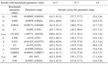
Sensitivity Analysis

37

increase in MPB-induced tree mortality changes for a 5% change in each parameter value (Table A1).

TABLE A1

Sensitivity of model results to a 5% change in parameter values

% decrease in maximum MPB-induced tree mortality due to the absence of:

Climate change Preference change Fire suppression

Results with benchmark parameter values 61.5 37.7 5.6

Benchmark parameter

values

Parameter range Results across the parameter range

δX 0.001 (0.00095, 0.00105) (61.5, 61.5) (37.7, 37.7) (5.6, 5.6)

δY 0.004 (0.0038, 0.0042) (63.1, 60.0) (38.3, 37.3) (6.0, 5.2)

bY 0.0018 (0.00171, 0.00189) (61.9, 61.1) (38.0, 37.6) (5.7, 5.5)

bA 0.1 (0.095, 0.105) (63.7, 59.3) (38.3, 36.9) (6.5, 5.3)

a1960 157,653 (149771, 165536) (60.6, 62.3) (37.3, 38.2) (5.6, 5.6)

φ 4,500 (4275, 4725) (62.3, 60.7) (38.2, 37.3) (5.6, 5.6)

d 0.015 (0.01425, 0.01575) (60.4, 62.8) (37.8, 37.9) (5.3, 6.1)

ν 0.5 (0.475, 0.525) (65.2, 54.3) (35.9, 37.0) (8.0, 2.3)

ρ 0.03255 (0.0309, 0.0342) (61.4, 61.6) (36.0, 39.5) (5.6, 5.6)

z 0.00054 (0.00051, 0.00057) (61.3, 61.7) (37.6, 37.8) (5.5, 5.7)

I1960 100 (95, 105) (63.3, 59.8) (38.1, 37.2) (7.1, 4.9)

β 0.96 (0.9597, 0.9634) (61.5, 61.5) (37.8, 37.7) (5.6, 5.6)

Notes. The percentage decreases sum to slightly more than 100% due to the interaction effects of climate change, preferences, and fire suppression.

Acknowledgements

38 References

Aadland, D. 2004. "Cattle cycles, heterogeneous expectations and the age distribution of capital."

Journal of Economic Dynamics and Control 28 (10): 1977-2002.

Aadland, D., C. Sims and D. Finnoff. 2011. "Mountain Pine Beetle Epidemics: Spatial Dynamics with Optimal Forest Management." Unpublished manuscript, Utah State University. Abbott, B., B. Stennes and G. C. van Kooten. 2008. "An Economic Analysis of Mountain Pine

Beetle Impacts in a Global Context." Unpublished manuscript, Department of Economics; University of Victoria.

Adams, D. M., C. S. Binkley and P. A. Cardellichio. 1991. "Is the Level of National Forest Timber Harvest Sensitive to Price?" Land Economics 67 (1): 74-84.

Alig, R., D. Adams, B. McCarl, J. M. Callaway and S. Winnett. 1997. "Assessing Effects of Mitigation Strategies for Global Climate Change with an Intertemporal Model of the U.S. Forest and Agriculture Sectors." Environmental and Resource Economics 9 (3): 259-274. Allen, C. D., M. Savage, D. A. Falk, K. F. Suckling, T. W. Swetnam, T. Schulke, P. B. Stacey, P.

Morgan, M. Hoffman and J. T. Klingel. 2002. "Ecological restoration of southwestern ponderosa pine ecosystems: A broad perspective." Ecological Applications 12 (5): 1418-1433.

Amacher, G. S., A. S. Malik and R. G. Haight. 2005. "Not Getting Burned: The Importance of Fire Prevention in Forest Management." Land Economics 81 (2): 284-302.

39

Aukema, B. H., A. L. Carroll, Y. Zheng, J. Zhu, K. F. Raffa, R. D. Moore, K. Stahl and S. W. Taylor. 2008. "Movement of outbreak populations of mountain pine beetle: influences of spatiotemporal patterns and climate." Ecography 31 (3): 348-358.

Azariadis, C. 1993. Intertemporal Macroeconomics. Cambridge, MA: Blackwell Publishers. Bengston, D. N. 1994. "Changing Forest Values and Ecosystem Management." Society and

Natural Resources 7: 515-533.

Bentz, B. 2006. "Mountain pine beetle population sampling: inferences from Lindgren

pheromone traps and emergence cages." Canadian Journal of Forest Research 36: 351-360.

Berck, P. 1979. "The Economics of Timber: A Renewable Resource in the Long Run." The Bell Journal of Economics 10 (2): 447-462.

Berryman, A. A., B. Dennis, K. F. Raffa and N. C. Stenseth. 1985. "Evolution of optimal group attack, with particular reference to bark beetles (Coleoptera: Scolytidae)." Ecology 66 (3): 898-903.

Bradshaw, K. M. and D. Lueck, eds. 2011. Wildfire Policy: Law and Economics Perspectives. Washington, DC: Resources for the Future Press.

Calkin, D. E., K. M. Gebert, G. Jones and R. P. Neilson. 2005. "Forest Service Large Fire Area Burned and Suppression Expenditure Trends, 1970-2002." Journal of Forestry 103 (4): 179-183.

40

Daigneault, A. J., M. J. Miranda and B. Sohngen. 2010. "Optimal Forest Management with Carbon Sequestration Credits and Endogenous Fire Risk." Land Economics 86 (1): 155-172.

Durlauf, S. N. and H. P. Young, eds. 2001. Social Dynamics (Economic learning and social evolution). Cambridge, MA: MIT Press.

Englin, J., P. Boxall and G. Hauer. 2000. "An Empirical Examination of Optimal Rotations in a Multiple-Use Forest in the Presence of Fire Risk." Journal of Agricultural and Resource Economics 25: 14-27.

Englin, J. and J. M. Callaway. 1993. "Global climate change and optimal forest management."

Natural Resource Modeling 7 (3): 191-202.

Fowells, H. A. 1965. Silvics of forest trees of the United States: United States Department of Agriculture.

Gibson, K. and J. F. Negron. 2009. "Fire and Bark Beetle Interactions." In The Western Bark Beetle Reserach Group: A Unique Collaboration with Forest Health Protection, eds. Hayes, J. L. and J. E. Lundquist, 51-70. Portland, OR: United States Department of Agriculture, Forest Service.

Gorte, R. W. 1994. "Lumber prices - 1993." In Report for Congress. Washington, DC: Congressional Research Service.

Hann, W. J. and D. L. Bunnell. 2001. "Fire and land management planning and implementation across multiple scales." International Journal of Wildland Fire 10: 389-403.

41

Heavilin, J. and J. Powell. 2008. "A novel method of fitting spatio-temporal models to data, with applications to the dynamics of mountain pine beetles." Natural Resource Modeling 21 (4): 489-524.

Holling, C. S. 1959. "The components of predation as revealed by a study of small predation of the European pine sawfly." Canadian Entomologist 91: 30.

Holmes, T. P., J. P. Prestemon and K. L. Abt, eds. 2008. The Economics of Forest Disturbances: Wildfires, Storms and Invasive Species. Springer.

Jenkins, M. J., E. Hebertson, W. Page and C. A. Jorgensen. 2008. "Bark beetles, fuels, fires and implications for forest management in the Intermountain West." Forest Ecology and Management 254 (1): 16-34.

Koch, P. 1996. Lodgepole Pine in North America: Forest Products Society.

Konoshima, M., C. A. Montgomery, H. J. Albers and J. L. Arthur. 2008. "Spatial-endogenous fire risk and efficient fuel management and timber harvest." Land Economics 84 (3): 449-468.

Kurz, W. A., C. C. Dymond, G. Stinson, G. J. Rampley, E. T. Neilson, A. Carroll, T. Ebata and L. Safranyik. 2008. "Mountain pine beetle and forest carbon feedback to climate change."

Nature 452 (24): 987-990.

Logan, J. A. and J. Powell. 2001. "Ghost forests, global warming and the mountain pine beetle."

American Entomologist 47: 160-173.

42

Logan, J. A., J. Regniere and J. A. Powell. 2003. "Assessing the impacts of global warming on forest pest dynamics." Frontiers in Ecology and the Environment 1 (3): 130-137. Lotan, J. E. and W. B. Critchfield. 1990. Pinus contorta Dougl. ex Loud. Department of

Agriculture.

Lubowski, R. N., A. J. Plantinga and R. N. Stavins. 2006. "Land-use change and carbon sinks: Econometric estimation of the carbon sequestration supply function." Journal of Environmental Economics and Management 51 (2): 135-152.

Mas-Colell, A., M. D. Whinston and J. R. Green. 1995. Microeconomic Theory. New York: Oxford University Press.

Murray, B. C. and D. N. Wear. 1998. "Federal Timber Restriction and Interregional Arbitrage in U.S. Lumber." Land Economics 74 (1): 76-91.

Newell, R. G. and R. N. Stavins. 2000. "Climate Change and Forest Sinks: Factors Affecting the Costs of Carbon Sequestration." Journal of Environmental Economics and Management

40 (3): 211-235.

O'Toole, R. 2006. "Money to Burn: Wildfire and the Budget." In The Wildfire Reader, A Century of Failed Forest Policy, ed. Wuerthner, G.: Island Press.

Parker, T. J., K. M. Clancy and R. L. Mathiasen. 2006. "Interactions among fire, insects and pathogens in coniferous forests of the interior western United States and Canada."

Agricultural & Forest Entomology 8: 167-189.

43

Peterson, G. D. 2002. "Contagious Disturbance, Ecological Memory, and the Emergence of Landscape Pattern." Ecosystems 5 (4): 329-338.

Phillips, B. R., J. A. Breck and T. J. Nickel. 2007. "Managing the economic impacts of mountain pine beetle outbreaks in Alberta." In Information Bulletin. Edmonton, Alberta: Western Centre for Economic Research.

Powell, J. and B. Bentz. 2009. "Connecting phenological predictions with population growth rates for mountain pine beetle, an outbreak insect." Landscape Ecology 24 (5): 657-672. Reed, W. J. 1984. "The effects of the risk of fire on the optimal rotation of a forest." Journal of

Environmental Economics and Management 11 (2): 180-190.

Romme, W. H., J. Clement, J. Hicke, D. Kulakowski, L. MacDonald, T. Schoennagel and T. Veblen. 2006. "Recent Forest Insect Outbreaks and Fire Risk in Colorado Forests: A Brief Synthesis of Relevant Research." Fort Collins, CO: Colorado Forest Restoration Institute.

Row, C., H. F. Kaiser and J. Sessions. 1981. "Discount rate for long-term Forest Service investments." Journal of Forestry 79: 367-369.

Runkle, J. R., ed. 1985. Disturbance regimes in temperate forests. New York: Academic Press. Safranyik, L. and A. Carroll. 2006. "The biology and epidemiology of the mountain pine beetle

in lodgepole pine forests." In The Mountain Pine Beetle: A Synthesis of Its Biology, Management and Impacts on Lodgepole Pine, eds. Safranyik, L. and B. Wilson, 3-66. Victoria, British Columbia: Canadian Forest Service, Pacific Forestry Centre, Natural Resources Canada.

44

Schoennagel, T., T. T. Veblen and W. H. Romme. 2004. "The Interaction of Fire, Fuels, and Climate across Rocky Mountain Forests." Bioscience 54 (7): 661-676.

Sedjo, R. A. 1995. "Ecosystem management: an uncharted path for public forests." Resources

121: 10,15-20.

Sims, C., D. Aadland and D. Finnoff. 2010. "A Dynamic Bioeconomic Analysis of Mountain Pine Beetle Epidemics." Journal of Economic Dynamics and Control 34 (12): 2407-2419. Smith, W. B., P. D. Miles, C. H. Perry and S. A. Pugh. 2009. Forest Resources of the United

States, 2007. Gen. Tech. Rep. WO-78. USDA Forest Service.

Sohngen, B. and R. Mendelsohn. 2003. "An optimal control model of forest carbon sequestration." American Journal of Agricultural Economics 85 (2): 448-457.

Taylor, S. and A. Carroll. 2004. "Disturbance, forest age, and mountain pine beetle outbreak dynamics in BC: a historical perspective." In Mountain Pine Beetle Symposium: Challenges and Solutions, eds. Shore, T. L., J. E. Brooks and J. E. Stone, 41–51. Kelowna, British Columbia: Natural Resources Canada Report BC-X-399.

Van Wagner, C. E. 1977. "Conditions for the Start and Spread of Crown Fire." Canadian Journal of Forest Research 7 (1): 23-34.

Wear, D. N. and B. C. Murray. 2004. "Federal timber restrictions, interregional spillovers, and the impact on US softwood markets." Journal of Environmental Economics and

Management 47 (2): 307-330.

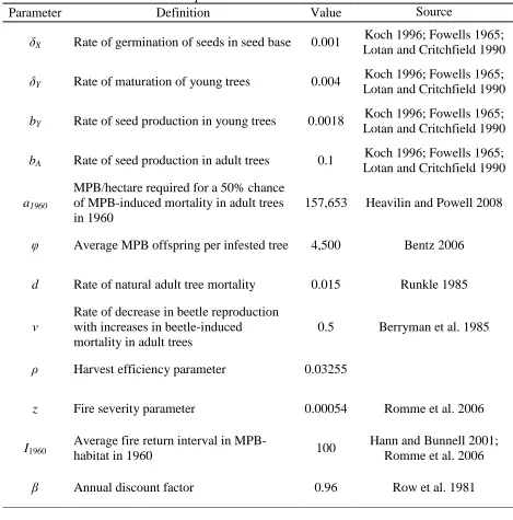
45 TABLE 1

Model parameters and initial condition

Parameter Definition Value Source

δX Rate of germination of seeds in seed base 0.001 Koch 1996; Fowells 1965; Lotan and Critchfield 1990

δY Rate of maturation of young trees 0.004 Koch 1996; Fowells 1965; Lotan and Critchfield 1990

bY Rate of seed production in young trees 0.0018 Koch 1996; Fowells 1965; Lotan and Critchfield 1990

bA Rate of seed production in adult trees 0.1 Koch 1996; Fowells 1965; Lotan and Critchfield 1990

a1960

MPB/hectare required for a 50% chance of MPB-induced mortality in adult trees in 1960

157,653 Heavilin and Powell 2008

φ Average MPB offspring per infested tree 4,500 Bentz 2006

d Rate of natural adult tree mortality 0.015 Runkle 1985

ν Rate of decrease in beetle reproduction with increases in beetle-induced mortality in adult trees

0.5 Berryman et al. 1985

ρ Harvest efficiency parameter 0.03255

z Fire severity parameter 0.00054 Romme et al. 2006

I1960

Average fire return interval in

MPB-habitat in 1960 100

Hann and Bunnell 2001; Romme et al. 2006

β Annual discount factor 0.96 Row et al. 1981

Initial condition corresponding to 1960 USDA FS harvest data

π 0.3% B 8,397 beetles/hectare

X 57,160 seeds/hectare Y 4,082 trees/hectare

46 FIGURE 1

Public forestland management and climate change as primary drivers of MPB outbreaks. Average annual temperature (A) and hectares burned (B) for 11 contiguous western states. (C) Billion board feet of green timber sold in USDA FS regions 1-6. (D) Hectares infested by MPB

47 FIGURE 2

Shift in preferences implied by USDA FS harvest data. Preferences for non-timber ecosystems services 𝛼_𝑡 are measured from the first-order condition in [11] and [13] with USDA FS timber

48 FIGURE 3

Simulation results from 1990 to 2008 using annual USDA FS timber sales data as proxy for harvests. Model results ignoring the effects of climate change (dotted line) yield MPB-indu