Ozone in the Stratosphere:
An Environmental Accumulation and Flow
Ronald C. Persin
College of Education – Florida Atlantic University | Boca Raton, FL 33431
(E-mail: [email protected])
Abstract: This article is concerned with the derivation of a set of differential equations that may contribute to the understanding of the formation of the ozone layer in the stratosphere. In the stratosphere, at an elevation extending from 10 to 50 kilometers, is where the planet's naturally occurring ozone gas filters the sun's ultraviolet (UV) radiation. Ozone abundances in the stratosphere seem to be determined by the balance between chemical processes that produce ozone and processes that destroy ozone. This balance is itself determined by the concentrations of reacting gases and how the rate or effectiveness of the various reactions varies with sunlight intensity (photon flux), location in the atmosphere, temperature, and other factors.
Key Words: Chapman reactions, photochemistry, photon flux, Beer’s Law.
BACKGROUND
Ecological models of environmental systems that utilize mathematical methods use equations to describe behavior. The equations are then applied to (i) an accumulation and flow, or (ii) a feed-back loop [1]. The amount of ozone that accumulates in the stratosphere is determined by the interaction of oxygen (O2) and light intensity (photon flux) from the Sun.
At this point in the project, oxygen-only chemistry will be used to estimate the ozone layer. Oxygen serves as both a creator and destroyer of ozone, according to the following equations:
The above equations represent the first successful attempt to quantitatively understand the photochemistry of ozone by S. Chapman in 1930 [2]. He proposed that O3 is created
by the dissociation of O2 to form O atoms, followed by the
reaction between O and O2. The workings of the
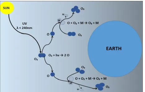
production equations are illustrated in Figure 1.
Fig 1. The Production of Ozone Based on the
Chapman Reactions.
Most of the photolysis of O2 in the stratosphere occurs at
wavelengths in the Schumann-Runge bands (175-200 nm) and the Hertzberg continuum (extending to 242 nm) [3].
The Chemist
O3 is destroyed by ultraviolet photons or the direct
reaction between O3 and O:
In addition to these, Chapman discussed several other reactions now known to be unimportant. The set of reactions, (1.1) to (1.5), known as the Chapman reactions, form the cornerstone of stratospheric O3 chemistry [4].
Considering just the Chapman reactions, the lifetimes 1/L of O3 and O for typical mid-latitude lower-stratospheric conditions are 1000 seconds and .002 seconds, respectively. The loss of O3 is dominated by photolysis, while the loss of O atoms is dominated by reaction with O2 to form O3.
The lifetime of O3 is 103 – 106 times greater than the lifetime of O in the stratosphere. Other constituents have lifetimes of days, weeks, months, or longer, many orders of magnitude longer than the lifetime for O3. In addition, many phenomena of interest, such as the Antarctic ozone hole, mid-latitude trends, and perturbations from volcanoes, occur on time-scales of months to decades. As a result, the “ozone” problem involves time-scales ranging over 15 orders of magnitude. This leads to both conceptual and computational difficulties [5].
While O2 is the only element that produces ozone, there are many other elements that destroy ozone. Most O3 destruction takes place through catalytic processes rather than the Chapman Reactions. Ozone is a highly unstable molecule that readily donates its extra oxygen molecule to free radical species such as nitrogen, hydrogen, bromine, and chlorine. An example of a depletion equation of this type would be:
Since oxygen, O2, is the only component of air that produces ozone (by photochemical and chemical reactions), this model, at first, will center on the O2 molecule. The O2 molecule consumes light energy to form ozone, so a model must be built for light intensity (photon flux) as a function of altitude by looking at how the presence of O2 affects incoming light intensity from the
sun.
PRESSURE AS A FUNCTION OF ALTITUDE
We now turn our attention to the derivation of an equation for air pressure as a function of altitude, which will be used to obtain an equation for oxygen concentration as a function of altitude. It is this oxygen that is critical to the formation of ozone. Although it is fairly obvious that temperature varies with altitude, for the purposes of this project it will be assumed that temperature remains constant. Specifically, let’s assume that the air temperature is 285 Kelvin, which is an estimate of the global average air temperature near the surface of the earth.
We know that the pressure exerted by a gas or fluid varies directly with altitude and the density. Atmospheric chemists refer to the mathematical relationship describing this phenomenon as the barometric equation. The barometric equation states that the rate of change in pressure, P, relative to altitude, a, is proportional to the density, , rho (mass per unit volume) of the fluid (in this case, air) where the proportionality constant is the negative of the acceleration due to gravity, g:
Now, using the Ideal Gas Law, which states that:
where:
V is volume measured in m3,
T is the temperature at the earth's surface measured in Kelvins (K),
P is pressure measured in kg / (m sec2) (also referred
to as newtons / m2),
n is the number of moles of gas (1 mole = 6.022 x 10²³
molecules), and
R is the gas constant measured in m2kg /
(sec2·K·mole).
Note that m/V is the definition of density and is denoted as .
Since we are formulating an expression for the density of air, which is a mixture of several gases, we will use an average molecular weight of air, Mair, which we will
calculate shortly. Mair is measured in kg/mole. We will
assume for the purposes of this project that g, R, Mair, and
T are constant relative to altitude.
The previous assumptions do not appear to be too far-fetched since most ozone is present at between 10-40 km altitude. All that is left is to solve the differential equation to obtain an expression for P(a) describing pressure as a function of altitude. We now have,
After separation of variables, integrating, and evaluating the constant, we get a result
with P0 = 1.013 x 10⁵ N/m2 , representing the initial
pressure which is the pressure at the Earth's surface (a = 0). Now let:
Atmospheric chemists refer to the combined parameter H as the scale height. Recall that the pressure (and thus, density) of air decreases with increasing altitude. The scale height, H, can be thought of as the height the entire atmosphere would have if its density were constant at the sea level value throughout.
We can compute the scale height, H, by determining the values of each of its parameters. Mair can be calculated
from the fractional composition and the molecular weight of each component in the air by taking a weighted average. Table 1, below, lists the significant chemical components of air along with their individual fractional amounts [6] and molecular weights [7].
Table 1: Average composition of the most
abundant gases in the atmosphere
Gases Fraction of Air M (kg/mole)
N2 0.78080 0.028013
O2 0.20950 0.031999
Ar 0.00930 0.029948
CO2 0.00034 0.044010
The values shown in Table 1 are those for the most abundant gases in dry air. It is understood that atmospheric air also contains water vapor. The amount of water vapor can vary from place to place, but the concentration of water vapor decreases with altitude, and above an altitude of about 10 km, atmospheric air consists of only dry air [8]. Therefore, the presence of water vapor in the atmosphere, particularly in the stratosphere, is being neglected.
If we assume that near the earth's surface the global average air temperature is 285 K, the gas constant, R, is 8.3144 m2kg/(sec2 K Mol), and the acceleration of gravity,
g, is 9.80 m/s2 then H 8400 m. So we now have the
equation for pressure as a function of altitude as:
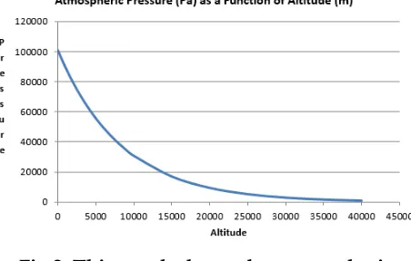
According to this equation, the pressure would drop in a logarithmic fashion as altitude increases. Up to 40 km, we have 99% of atmospheric mass, and the upper boundary at which gases disperse into space is approximately at 1000 km above sea level. A plot of the above equation is shown in Figure 2.
Fig 2. This graph shows that atmospheric
pressure decays exponentially from its value
OXYGEN AS A FUNCTION OF ALTITUDE
Now we shift our focus from pressure as a function of altitude to concentration of oxygen as a function of altitude. To accomplish this, it is assumed that pressure and concentration of oxygen can be related through the Ideal Gas Law:
The left hand side, , is in moles / m3 but
atmospheric chemists seem to prefer to work in units of (molecules / m3), so the concentration quantity from the
above equation should be multiplied by Avogadro's number, 6.022 x 10²³ (molecules / mole). Additionally, not
every air molecule is an oxygen molecule, O2, so in order
to obtain an expression for concentration of O2 , we also
need to multiply the concentration of air by the fractional abundance of O2 in the air, which is 0.2095 (given in Table
1).
We can now express C(a) as the concentration of oxygen at a given altitude by the following equation:
Here, Co represents the concentration of O2 at altitude
a = 0, sea level.
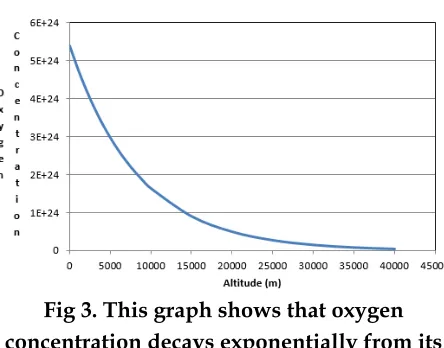
The results of this derivation are illustrated as a plot in Figure 3, which shows that the concentration of oxygen decays exponentially from its value at the surface of Earth.
Fig 3. This graph shows that oxygen
concentration decays exponentially from its
value at the surface of Earth
FORMULATION OF A DIFFERENTIAL
EQUATION FOR PHOTON FLUX I
AS A FUNCTION OF ALTITUDE
Let us consider passing light of a single wavelength through a substance that tends to absorb light. It makes sense from a qualitative point of view that the intensity of the light (or photon flux) should diminish as the light travels through the substance. In essence, the more light-absorbing molecules with which the incident light comes into contact, the more the light intensity decreases.
There are two important parameters that determine how many light-absorbing molecules a given incident light will contact. The first is the concentration of the absorbing molecules. As the concentration increases, the light intensity will be attenuated by a greater amount. The second parameter is the length of the path the light takes through the absorbing medium. As the path length increases, the light will come into contact with more absorbing molecules, and thus the light intensity will diminish.
There is yet another term that greatly affects how light is absorbed by a substance. In this report, the term is called the absorption cross section, σ. This term can be thought of as the ability of a particular molecule to absorb light of a certain wavelength.
To formulate a differential equation that examines the change in photon flux relative to change in altitude, we use a form of Beer's Law, which states that the rate of change in photon flux relative to altitude is the product of the amount of photon flux present, the concentration of light absorbing species present at a particular altitude, and the ability of the absorbing species to absorb light of a certain wavelength. This is described by the differential equation:
where,
I(a) = photon flux at altitude, a
C(a) =concentration of absorbing species at altitude, a
σ = absorption cross section of the absorbing species.
altitude, a, and assumes that the only absorber of light is the oxygen molecule, O2.
Now we chose 240 nm as the wavelength of light for our model because it is in the ultraviolet range of light where oxygen absorbs most readily. The value for the absorption cross section of O2 at this wavelength is 1.0 x
10-28 m2 [9]. The photon flux from the sun at this
wavelength, I0, is 7.61 x 10¹⁷ photons/(m2sec).
Now we combine Beer's Law with our previous equation for C(a) and use separation of variables to solve for I(a). The initial condition is that I(a) = I0 when a →∞
(top of the atmosphere). Therefore, we get:
where:
I = amount of light with absorber present
Io = amount of light with no absorbers
σ = absorption cross section (m2/molecule)
H ≈ 8400 m, scale height
a = altitude
k = e(-σ·C0·H) ≈.01072
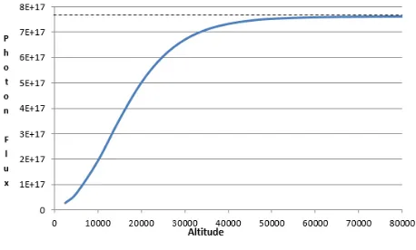
The results of this derivation are shown as a plot in Figure 4. Solar photon flux is increasing with altitude from the surface of Earth to its maximum value at Io.
Fig 4. This graph shows photon flux as a
function of altitude, for a single 240 nm
wavelength, asymptotically approaching I
o.
SUMMARY & CONCLUSION
Ozone abundances in the stratosphere are determined by the balance between chemical processes that produce ozone and processes that destroy ozone. This balance is
itself determined by the amounts of reacting gases and how the rate or effectiveness of the various reactions varies with sunlight intensity (photon flux), location in the atmosphere, temperature, and other factors.
As we examine the graphs of oxygen concentration and photon flux, both as functions of altitude, reasons for the abundance of ozone in the stratosphere seem to be apparent. It is in this layer of the atmosphere, between 10,000 and 50,000 meters, that the conditions for ozone formation are maximized. At higher altitudes there is apparently not oxygen available for this reaction to take place. As for lower levels, the photolysis of oxygen is dependent on the availability of very short-wave sunlight and in lower layers of the stratosphere there is a shortage of the necessary short wavelength light because much of it is absorbed higher up in the atmosphere. Oxygen, O2,
consumes light energy and it does this most efficiently at 240 nm to form ozone, O3. The mechanism for
stratospheric ozone formation, photolysis of O2, does not
take place in the troposphere because the strong UV photons needed for this photolysis have been absorbed by O2 and ozone in the stratosphere. It is this process (as well
as others that are not part of this project) that allows ozone in the stratosphere to be maintained, and subsequently to filter-out ultraviolet radiation.
For activities to help students understand the importance of the ozone layer, as well as its formation and depletion, several references [10,11,12,13] are provided.
REFERENCES
1. Miller GT, Jr. in Living in the Environment, Ninth Edition, Wadsworth Publishing Company, Belmont, CA, 1996, pp 3, 56-59.
2. Chapman S. A theory of upper-atmospheric ozone, Mem. R. Meteorol. Soc., 1930, 3, 103-125.
3. Minschwaner K, Salawitch RJ, McElroy MB. Absorption of solar radiation by O2: implications for O3 and lifetimes of N20, CFC13 and CF2C12, J. Geophys. Res., 1993, 98, 10,543-10,561.
4. Dobson GMB. Forty years’ research on atmospheric ozone at Oxford: a history, Appl. Opt., 1968, 7, 387-405. 5. Dessler A in The Chemistry and Physics of
Stratospheric Ozone, First Edition, Academic Press, San Diego, CA, 2000.
6. Pidwirny M. "Atmospheric Composition". Fundamentals of Physical Geography, 2nd Edition,
http://www.physicalgeography.net/fundamentals/7 a.html
7. Tyson PJ.. "The Kinetic Atmosphere: Molecular Masses", 2012. Retrieved from: www.climates.com/KA/BASIC%20PARAMETERS/
molecularmasses.pdf
8. Gabor M. “Water Vapor From Satellite Based GPS Receivers”, (n.d.). Retrieved from http://www.csr.utexas.edu/texas_pwv/midterm/ga bor/gpsspace.html
9. Yoshino K, et al. Planet. Space Sci., 1988, 36, 1469-1475. Retrieved from rpw.chem.ox.ac.uk/JPL_02-25_5_photochem_rev01.pdf
10.“Ozone Activities”. SERC Site Guides. Retrieved from http://www.ucar.edu/learn/1_1_1.htm
11.“Ozone Attack”. Student Activities. Retrieved from http://serc.carleton.edu/serc/site_guides/ozone_acti vities.html
12.“SAM II – Disappearing Ozone”. Activity #3. Retrieved from
http://www.esrl.noaa.gov/gsd/outreach/education /samii/SAMII_Activity3.html
13.NASA. “Ozone Hole Watch”. Retrieved from http://ozonewatch.gsfc.nasa.gov/education/SH.html