Studies in crop variation. VIII. An application of the resistance formula to potato data

Patron: Her Majesty The Queen Rothamsted Research Harpenden, Herts, AL5 2JQ

Telephone: +44 (0)1582 763133 Web: http://www.rothamsted.ac.uk/

Rothamsted Repository Download

A - Papers appearing in refereed journals

Kalamkar, R. J. 1930. Studies in crop variation. VIII. An application of the

resistance formula to potato data. The Journal of Agricultural Science. 20

(3), pp. 440-454.

The publisher's version can be accessed at:

•

https://dx.doi.org/10.1017/S002185960000695X

The output can be accessed at:

https://repository.rothamsted.ac.uk/item/9703w/studies-in-crop-variation-viii-an-application-of-the-resistance-formula-to-potato-data

.

© Please contact library@rothamsted.ac.uk for copyright queries.

VIII. AN APPLICATION OF THE RESISTANCE FORMULA TO POTATO DATA.

BY R. J. KALAMKAR, B.Sc, B.AGR.

Statistical Department, Rothamsted Experimental Station, Harpenden.)

I. INTRODUCTION.

A MATHEMATICAL expression called the Resistance Formula which formu-lates a yield-factor relationship as suggested by Maskell has been critically tested by Bhai Balmukand(i). The formula postulates that the reciprocal of the yield is the sum of portions, each a function of one nutrient, such as F (N), F' (K), etc. Further, the function of a particular nutrient is inversely proportional to that nutrient in an available form. Based on this hypothesis, the equation for the yield y can be represented thus:

- = F (N) + F' (K) + F" (P) + ..., etc.,

where F {N) = - ^ , F' {K) = 7 - ^ ,

Art I ^VI * IA I Mjt

an, ak, etc. being the constants varying with the nutrient and the crop;

n and k represent the available nitrogen and potash in the unmanured

soil, and N and K the Quantities added.

n and k represent the available nitroge

soil, and N and K the quantities added

II. MATERIAL AND METHOD OF INVESTIGATION.

The object of this paper is to make a further test of the validity of the Resistance Formula, and use is made of the Rothamsted Potato Experiment on Long Hoos Field, Section I, in 1929. This experiment was designed to give information as to the effect on yield of applying nitrogenous, potassic and phosphatic fertilisers in various quantities. There was a basal dressing of dung at the rate of 14 tons per acre and further nitrogen was supplied as sulphate of ammonia at rates of 0, 0-3 and 0-6 cwt. of nitrogen and potash in the forms of sulphate, muriate and potash manure salts at rates equivalent to 0, 0-5 and 1 cwt. of K2O per acre. Superphosphate was applied at the rate of 04 cwt. of

P2O5 per acre. The experiment consisted of 81 plots arranged in nine

E. J. KALAMKAR 441

block was equalised with respect to tlie different kinds of potassic fertilisers, i.e. the three plots having single potash had it in the forms of sulphate, muriate and potash salts respectively, and likewise the doubly dressed plots, and each set of these blocks, taken by row or by column, had complete replication both quantitatively and qualitatively for the potash comparison. As for the application of phosphate, each plot was divided into two sub-plots, only one of which, chosen at random, received superphosphate. The area of each sub-plot was 1/90 acre. Analysis showed that the response to potash dressings was the same for all the different qualities, and their yields have, therefore, for present purposes been averaged, yielding Table I below.

Table I. Potatoes (Ally) Long Hoos, Section I, 1929. Average yield in tons per acre (y).

Cwt. of K,0 per acre

0 0-5 1 0

Mean Reciprocal

Without phosphate (cwt. oi

0 '

4-52 4-86 4-62

: nitrogen per

0-3 5 1 0

5-26 5-30

5 1 2

019531

• acre)

0-6 5-38 5-41 5-59

(cwt.

i

0 4-79

5 0 1

4-89

i (difference) = 000869

With phosphate of nitrogen per acre)

0-3

5-52 5-90 5-77 5-62 017793

0-6

5-94 6-28 6-51

Now, the measurement of agreement of the expected yields with those observed affords us a means of judging the accuracy of any hypo-thesis to be tested. I t is therefore necessary to obtain values of the expected yields obeying the Resistance Formula and approximating to the observed.

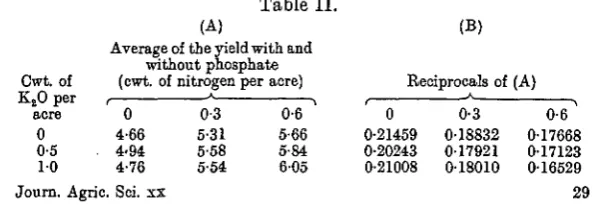
Crude values of the reciprocals of the expected yields based on the Resistance Formula were first arrived at by averaging the yields obtained for each combination of N and K with an d without phosphate, finding their reciprocals and adding to and subtracting from them half the difference of the reciprocals of the means of yields obtained with and without phosphate. This was done by means of the following table.

Table I I .

(A) (B) Average of the yield with and

without phosphate

Cwt. of (cwt. of nitrogen per acre) Reciprocals of (A) Ks0 per

Table III. Reciprocals of the expected yield 1/m built up by adding to and

subtracting 0-00869 from the reciprocals in Table II (B).

Without phosphate

A

f \

0-22328 0-19701 018537 0-21112 0-18790 017992 0-21877 018879 017398

Mean (6) 0-21772 019123 017976

Mean (o) 0-20189 019298 019385 With phosphate

0-20590 017963 016799 019374 017052 016253 0-20139 017141 0-15660 0-19624 (c) (6)0-20034 0-17385 0-16237

Mean (a) 018451 017560 0-17647 0-17886 Mean(c)

Table IV (A). Reciprocals of the expected yields buili up from the margins of Table III by use of summation formula a + b — c.

Without phosphate With phosphate

0-22337 0-21446 0-21535 019688 0-18797 018884 018541 017650 017735

0-20599 017950 016802 019708 017059 015911 019795 017146 015998

Table IV (B). Values of first approximation of m, i.e. reciprocals of

Table IV {A).

Without phosphate With phosphate

4-477 4-662 4-643 5-079 5-320 5-296 5-393 5-666 5-638 4-854 5074 5052 5-571 5-862 5-832 5-951 6-285 6-251

For the purpose of* improving these expectations we shall further need a table of m4.

Table IV (C). Values o/m4.

Without phosphate 402 472 465 Total 1339 666 801 787 2254 846 1030 1010 2886 Total 1914 2303 2262 6479 With 551 663 651 1865 Total 4682 5707 5596 phosphate A 963 1181 1157 3301 1254 1560 1526 4340 Total 2768 3404 3334 9506

3204 5555 7226 15985

These fourth powers of the crude expectations are then used as weights in obtaining the improved fit, for they are inversely proportional to the variances of the reciprocals in the field trial.

Table V. Reciprocals of the observed yields (1/y) from Table I. Without phosphate With phosphate

0-22124 0-20576 0-21645 019608 019011 018868 0-18587 0-18484 017889

E. J . KALAMKAR 443

The margins in the following tables are built up by taking the weighted averages of the reciprocals of the observed yields, for rows and columns separately (with and without phosphate) and for the combined tables.

Table VI (A). Weighted averages of the reciprocals of the observed yields.

Without phosphate

(6) 0-21412 019137 018306 (a) 0-19685 019096 019002

"With phosphate

019237 (c) (b) 0-20402 017423 015989 (a) 0-18085 017066 017038 0-17353 (c)

Table VI (B).

(b) 0-20824 018119 016914

(a) 018739 017885 017832 0-18117 (c)

The difference of 0-18117 from 0-19237 represents the correction to be applied to the margins of Table VI (B) to get the margins of Table VII (A) below. Likewise the difference of 0-18117 from 0-17353 represents the correction to be applied to the table to get the margins of Table VII (B). The individual nine values of each set are then obtained from the margins by the relation a + b — c.

Table VII. (A)

Without phosphate

0-22566 019861 018658 0-21712 019007 017802 0-21659 0-18954 017749 (6) 0-21944 019239 018034

(a) 019859 019005 0-18952

(B) With phosphate f ' \ 0-20682 017977 016772 019828 017123 015918 0-19775 017070 0-15865 019237 (c) (6) 0-20060 017355 016150

(a) 0-17975 0-17121 0-17068

0-17353 (c)

The margins of Table VI (B) are further improved by applying various corrections which are found by taking the weighted average difference between the reciprocals of the observed and expected values of Tables V and VII respectively. The arithmetic is much facilitated by preparing the following table.

Table VIII. Differences between the reciprocals of the observed and

expected values.

Without phosphate With phosphate

-000442 -001136 -000014

-000253 + 0-00004 -000084

-000069 + 000682 + 000140

+ 0-00295 + 0-00132 + 000675

+ 0-00139 -0-00174 + 000261

444

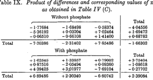
Table IX. Product of differences and corresponding values of m4

as obtained in Table IV (C).

Total

Total

-1-77684 -5-36192 -006510 - 7-20386

+ 1-62545 + 0-87516 + 4-39425 + 6-89486

Without phosphate

-1-68498 + 003204 -0-66108 - 2-31402

With phosphate

A

+1-33857 -205494 + 3.01977 + 2-30340

-0-58374 + 702464 +1-41400 + 7-85486

+ 0-79002 + 009360 -7-69104 - 6-80742

Total -404556 +1-69472 + 0-68782 -1-66302

Total + 3-75404

-1-08618 -0-27702 + 2-39084

Table X. Corrections obtained by adding margins of Table IX and dividing

by marginal m4 in Table IV (C), with and without phosphate combined.

-0-00010 000014

-000006 + 000011 + 0-00007

-000026 for plots without phosphate + 000025 for plots with phosphate

The value — 0-00026 is the quotient of — 1-66302 and 6479, while + 0-00025 is the quotient of + 2-39084 and 9506.

The improved values for the reciprocals of the expected yields after applying the corrections are shown in Table XI (A), e.g. 0-22524 (without phosphate) and 0-20691 (with phosphate) are obtained by adding - 0-00006, - 0-00010 and - 0-00026 to 0-22566 (without phosphate), and - 0-00006, - 0-00010 and + 0-00025 to 0-20682 (with phosphate) in Tables VII (A) and (B) respectively.

Table XI (A). Reciprocals^ the expected yields (1/m). Without phosphate With phosphate

0-22524 0-21687 0-21630

019829 0-18992 0-18955

018638 017801 017744

0-20691 019854 019797

017996 017159 017102

016805 015968 015911

Table XI (B). Values of m. Reciprocals of values in Table XI (A). Without phosphate With phosphate

, * , , * , 4-440 5043 5-365 4-833 5-557 5-951 4-611 5-265 5-618 5037 5-828 6-262 4-623 5-275 5-733 5054 5-847 6-285

R. J. KALAMKAR

445

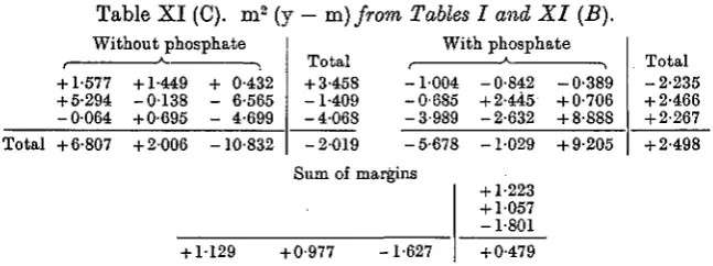
At this stage, two tests were applied to see how far the values of m as obtained in Table XI (B) supply a sufficient fit to the observed yields. If the process is sufficiently complete (i) S (y — m)2 should be approxi-mately at its minimum value; similarly (ii) Sm2 (y — m), taken over all

plots treated alike in respect to any one manure, must be small com-pared to the individual values of w2 (y — m).

Table XI (C). m2 (y - m) from Tables I and XI (B). Without phosphate

+ 1-577 + 5-294 - 0064 Total +6-807

+ 1-449 -0138 + 0-695 + 2006

+ 0-432 - 6-565 - 4-699 -10-832

Total + 3-458 -1-409 -4-068 -2019

With phosphate

-1004 -0-685 -3-989 -5-678

-0-842 + 2-445 -2-632 -1-029

-0-389 + 0-706 + 8-88S + 9-205

Total -2-235 + 2-466 + 2-267 + 2-498 Sum of margins

+ 1-129 + 0-977 -1-627

+ 1-223 + 1-057 -1-801 + 0-479

The marginal totals are fairly high when compared with the individual entries, and thus indicate that the values of m as obtained above are not yet sufficiently fitted to the observed yields. Consequently an im-proved fit of the values of m is now sought by the "Method of Least Squares."

It is required to minimise the quantity Q = S (y — m)2, where y stands for an observed yield and m may be expressed in terms of certain adjustable parameters which may be specified as follows:

where Pr takes the two values P and 0 according as the plot does not

or does receive phosphate;

Kg takes three values K, K' and 0 for none, single and double

potash;

Np takes three values N, N' and 0 for none, single and double

nitrogen.

Then m is obtained from the six arbitrary parameters C, P, K, K', N, Nr.

The equations to be satisfied on minimising are

dQ dQ dQ dQ dQ _ dQ

dC~dP~dK~dK' dN dN'

These are non-linear equations in six unknowns but, commencing with the approximate solution already obtained, the solution may be obtained by successive approximations.

suppose C — Co + c, P — Po + p, etc., where c, p, Jc, h', n and n' are the

corrections required. Then

() _dC~dC+

I I:' dQ 1 n * ° I n'

^ndCodKo ^ * dCodKo' T "dC0dN0 ^ dCodNo"

d*Q d*Q d*Q , d*Q P UK AP dK ' HP tJN HP tJN "

(iii, . g

-' -r J r/ J D T v j « - , « * J17 J7L1 ' JIX" J AT ' '

dQ _ dQ ~dK'~dK^' +

dQ dQ ,

d2Q

ic d*Q , h d*Q I y

(vi) Q ..

dNodPo + diVodGo di dQ d>Q d?Q

+ n + n

'~ dN0' + n dN0'* + n dNodNo'

P IW^JW + c +rj/~1 > JUT f J XT ' J AT 'Jit/' '' * + *' r0 u.x 0 u.i.v0 a o0 ajyo an.o azv0 a i i0

Thus we have six equations which are linear in c, p, k, k', n and n' with known coefficients, for

dQ o o . dm n1!, , . ., the summation being -jTv- = — 2/S (y — m) 37=- = 2<S {m3 (v — m)}, „ ,, . , , °

dC0 ^ ' dC0 i ^ IS over all the eighteen

plots;

dQ 9

Tp- = 25m2 (y — m) over plots without phosphate;

-Tjz- = 2£m2 (y — m) over plots without potash;

dQ 6

R J. KALAMKAR 447

dQ 6

-=-^~- = 2Smi (y — m) over plots without nitrogen;

— = 2Sm3 (y — m) over single nitrogen plots. dN0

These quantities can all be obtained readily from Table X I (C).

dH) „ d \f „ . > *,§, . „ , , ... summation

be--,-J% = 2 -JT^- £m2 (y- m) = 2S {m4 - 2m3 (y — m)} . ,. ,, dC<? dCoi " i * " ing over all the

eighteen plots;

d2Q 9

J = 25 {m4 — 2m3 (y — m)} over plots without phosphate; dLdF !

dzQ „ 5, , . „ , , Xs over plots without phosphate but . „ J L , = 2»S {m4 — 2m3 (y - m)} ... ^. . r , r, ,

dPodKo i w with smgle dressing of potash;

6

= 2/S {m4 — 2m3 (y — m)} over plots without potash; dCodKo i

and so on

d*Q d>Q dK0dK0' dNodNo' ~

dz0 d2Q °

The values of -JT^\, ,n iP ;

Q

te-> a re obtained from the following table:

Table X I I . m4 - 2m3 (y - m).

Without phosphate

374-637 632-166 823-828 403-209 769-857 1069-923 457-355 766-947 1134130 Total 1235-201 2168-970 3027-881

With phosphate

Total , " ,

1830-631 555-304 962-938 1258-787 2242-989 650-589 1125-184 1528-819 2358-432 692-766 1199-534 1448-610

6432052 1898-659 3287-656 4236-216

S u m of margins

4607-660 5547-581 5699-342

Total 2777029 3304-592 3340-910

9422-531

3133-860 5456-626 7264097 15854-583

The values of -^, -~i, ,~ Yp > •••> etc. when substituted in the

six equations enable them to be solved for c, p , k, k', n and »', with the following results:

c = - 0-000258; ' k' = + 0-000028;

p = + 0-000158; n=- 0-000160; k = - 0-000045; n' = + 0-000022.

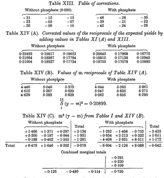
The table of corrections is then built up from the relation

where x takes the values p and o according as it is applied to plots without phosphate and plots with phosphate respectively. Similarly y takes the values k, k' and o for none, single and double potash; z takes the values n, n' and o for none, single and double nitrogen.

Table XIII. Table of corrections. Without phosphate (0000) With phosphate

-31 -23 -26

- 1 2 - 0 5 - 0 8

- 1 5 -07 - 1 0

- 4 6 - 3 9 - 4 2

- 2 8 - 2 1 - 2 4

- 3 0 - 2 3 - 2 6

Table XIV (A). Corrected values of the reciprocals of the expected yields by

adding values in Tables XI (A) and XIII.

Without phosphate With phosphate

0-22493 0-21664 0-21604 019817 0-18987 0-18927 018623 017794 0-17734 0-20645 0-19815 019755 017968 017138 0-17078 016775 015945 015885 Total

Table XIV (B). Values of m reciprocals of Table XIV (A). Without phosphate With phosphate

4-446 5-046 4-616 5-267 4-629 5-283 5-370 5-620 5-639 4-844 5047 5062 5-565 5-835 5-855 5-961 6-271 6-295 :

S (y - mf = 0-20899.

l

Table XIV (C). m2 (y - m)from Tables I and XIV (B). Without phosphate

f •*

+ 1-466 +1-371 +0-297 + 5-200 -0187 -6-944 -0-188 +0-462 -1-555 + 6-478 +1-646 -8-202

Total + 3134 -1-931 -1-281

With phosphate

-1-262 -1-408 -0-755 -0-934 +2-213 +0-332 -4-408 -2-931 +8-511 -0-078 -6-604 -2126 +8-088

Total - 3-425 + 1-611 + 1-172 -0-642

Combined marginal totals

-0126 -0-480 -0114

-0-291 -0-320 - 0 1 0 9 -0-720

The marginal totals are now much reduced, indicating that the value of m has been further improved.

Test of Goodness of Fit.

E. J. KALAMKAR 449

analysis of variance developed by Dr E. A. Fisher (2) is applied to test the validity of the hypothesis. From the analysis of variance for this experiment it is found that after apportioning, fractions of the total sum of squares of deviations of the yields from their general mean to various known causal factors, the following residual amounts are left for (i) the N and K error, and (ii) the phosphate error. (For aii explanation of a similar analysis but with only three blocks see Wish art and Clap-ham (3)).

Degrees of Sum of Mean Analysis of variance due to: , freedom squares square

(i) Non-adjacent sub-plots (N and t e r r o r ) . . . 60 23127818 3854-64 (ii) Adjacent sub-plots (phosphate error) ... 60 59271-89 987-86

These figures are based on the yields in J lb. units per l/90th of an acre. Expressed in tons per acre, the mean squares for non-adjacent and adjacent sub-plots are 0-38800 and 0-09968 respectively. But the yields in our tables are based on the means of nine sub-plots; so to make the figures comparable we have to divide them by nine. Thus

Analysis of variance due to:

(i) Non-adjacent sub-plots (N and K error)... (ii) Adjacent sub-plots (phosphate error)

There are seventeen degrees of freedom for the eighteen values of the table out of which five have been accounted for in fitting the con-stants, leaving twelve degrees of freedom in which the observed values might differ from expectations. The twelve degrees of freedom can further be split up into (i) eight for differences from expectation due to fertility of adjacent sub-plots, and (ii) four for the non-adjacent ones. The total sum of the squares of the deviations of the expected yields from the observed ones is

S(y- mf = 0-20899.

The sum of the squares of the deviations of the expected yields from the observed values for eight degrees of freedom due to fertility of adjacent sub-plots was calculated from the following tables.

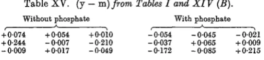
Table XV. (y - m)from Tables I and XIV (B).

Without phosphate With phosphate Degrees of

freedom

60 60

Sum of squares 2-5928 0-6648

Mean square 0-04321 001108

Table XVI. Differences, phosphate—no phosphate, of (y — m)

from Table XV. -0128 - 0 0 9 9 - 0 0 3 1 -0-281 +0072 +0-219 - 0 1 6 3 - 0 1 0 2 +0-264 £ (sum of squares of the above nine figures) =0-13270.

The difference of 0-13270 from 0-20899 represents the sum of t h e squares of the deviations of the expected yields from the observed values with four degrees of freedom for the non-adjacent plots.

If the Resistance Formula has' been satisfactorily fitted, the mean sum of squares with the eight degrees of freedom should not be signifi-cantly larger than t h a t obtained from the field error for the phosphate comparison; similarly, the mean square of deviations with four degrees of freedom should not be significantly larger than t h a t obtained for t h e

N and K comparison in the field experiment. We have:

Degrees of Sum of Mean £ loge (mean

Analysis of variance due to: freedom squares square square+ 100) (i) Eesistanoe formula 4 0-0763 0-01907 0-3227

Non-adjacent sub-plots {N and K error) 60 2-5928 0-04321 0-7317 In this case the mean square from the Resistance Formula is actually less than that for the corresponding field error, z = — 0-4090.

Degrees of Sum of Mean £ loge (mean

Analysis of variance due to: freedom squares square square+ 100) (ii) Resistance formula 8 01327 001659 0-2531

Adjacent sub-plots (P error) ... 60 0-6648 0-01108 0-0512 In this case, although the mean square of deviations for adjacent sub-plots is greater than the mean square for the corresponding field error, it is not significant, as is shown by the value of z. To reach the 5 per cent, point the value of z is required to be 0-3702. It is evident that the Resistance Formula has fitted the data satisfactorily in this case.

• III. CONSTANTS OF THE RESISTANCE FORMULA.

Bh. Balmukand has shown in the data examined by him that F (N),

F' (K), etc. can be taken to be of the form — " and r—^=, where

an and ak are the constants varying with the nutrient and the crop,

while n and k represent the available nitrogen and potash in the un-manured soil. The fitness of this special formula cannot be tested from our data, but the values of the constants n, an, k, ak are calculated by

R J. KALAMKAR 451

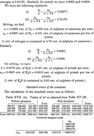
constants p and aP cannot be determined. From the Table XIV (A) we

find that the difference between the reciprocals of the expected yields for no nitrogen and 0-3 cwt. of nitrogen is practically 0-02677—any departure from constancy in the last place being really due to the neglect of the sixth decimal place—and that between those of 0-3 and 0-6 of nitrogen is 0-01193. Similarly for potash we have 0-0083 and 0-0006.

We have the following equations:

Solving, we find

n = 0-4823 cwt. of N2 = 2-305 cwt. of sulphate of ammonia per acre; an = 0-0337 cwt. of N2 = 0-161 cwt. of sulphate of ammonia per ton of

potato.

(1 cwt. of nitrogen is contained in 4-78 cwt. of sulphate of ammonia.) Similarly

On solving, we nave

k = 0-0779 cwt. of K2O = 0-157 cwt. of sulphate of potash per acre;

ak = 0-0007 cwt. of K20 = 0-0015 cwt. of sulphate of potash per ton of

potato.

(1 cwt. of K2O is contained in 2-02 cwt. of sulphate of potash.)

Standard errors of the constants.

The calculation of the standard errors was as follows:

Table XVII (A). Values of m* as obtained-from Table XV (B).

Without phosphate

390-671 648-405 831-382 453-988 769-452 997-480 461-559 779-242 1011056 Total 1306-218 2197-099 2839-918

Total

With phosphate

1870458 550-480 959-401 1262-843 2220-920 648-670 1159-205 1540-456 2251-857 656-584 1175-585 1570-553

6343-235 1855-734 3294191 4373-852 Total 2772-724 3348-331 3402-722

9523-777

Combined marginal totals

wnt 3161-952 5491-290 7213-770

w_nt

3161-952 5491-290 7213-770

Table XVII (B). n + Nt (cwt.

of sulphate of ammonia)

2-305 3-739 5173

n + Nt

1371-78 1468-65 1394-50

595-13 392-79 269-57

258-19 10505 5 2 1 1

112-01 28-10 10-77 Total 15867-012 — 4234-93 1257-49 415-35 150-88

Table XVII (C).

4643-182 5569-251 5654-579

K, (cwt.

of sulphate of potash)

0157 1167 2-177

w kt

29574-41 4772-28 2597-42

18837202 4089-36 119312

(k+Kty (k+Kty

1199821-80 764217711 350416 3002-71 548-06 251-75

Total 15867012 36944-11 193654-50 120387402 7645431-57

The values of the standard errors were obtained by using the formula given by Bh. Balmukand.

3 S- w.'nt

3

-s-u_nt

Nt)* 3

- S

1 I

3 Si,

1

w.nt

i (n + ^,)«

3

-

<s-

v_nt

i (n + Nt)*

3

- 5 w.'nt

(n +

i^

)

3

i S

-Nt)

3

- 5-

3

Nt)

3 w,'nt

w.'nt

3

f (n + N

)

I

where D is the denominator of the previous fraction. Substituting the respective values:

Similarly:

an — 01158 cwt. of sulphate of ammonia,

crOfi = 0-1182 cwt. of sulphate of ammonia.

CTW = 1-1552 cwt. of sulphate of potash,

a_a

R. J. KALAMKAR 453

Expressing the constants with their standard errors in lb. of nitrogen and K2O, we have:

n = 54-02, S.E. 2-71, k = 8-70, S.E. 64-05, an = 3-77, s'.s. 2-77, ak = 0-08, S.E. 0-68.

With the exception of n, for which the standard error is only 5 per cent., the standard errors we have obtained for the constants of the Resistance Formula are very high. The values of the constants together with their standard errors are set out in the following table and the results previously obtained by Bh. Balmukand, converted into pounds of nitrogen and K2O respectively, are added for comparison.

Long Hoos (Ally) 1929, dung (14 Stackyard (Kerr's Pink), 1926 Seale Hayne: dung (10 tons) ... Seale Hayne: undunged, 1927

Table XVIII. n

tons) 5402 ... 40-71 ... 38-89 ... 13-35

S.E.

2-71 19-91 9-37 5 1 5

a_n

3-77 2-31 3-96 1-85

S.E.

2-77 1-44 112 0-80

k 8-70 26-61 62-65 - 5 - 5 5

S.E.

64-05 33-27 3216 4-99

a

k 0 0 8 0-49 1-43 0-42

S.E.

0-68 0-71 0-94 0-35

IV. SUMMARY AND CONCLUSION.

The table of results given in the last section shows that for all experi-ments for which the Resistance Formula has been fitted the values of the constants are consistent, bearing in mind the standard errors to which these values are subject. The constants for nitrogen may be held to have been determined with some approach to precision, but those for potash are not so well determined. We find at Rothamsted, for example, that the crop responds to a moderate dressing of potash, but higher dressings do not usually improve the yields any further. This fact limits the precision of the formula. The reader is asked to refer at this point to the full descriptions as to the meaning to be attached to the constants of the formula given by Bh. Balmukand in the earlier paper (i). The constants an and ak, called the importance factors, are interpreted

as determining the capacity of the crop to recover the particular nutrient out of the soil. The chemical analysis of the tubers grown under nitrogen and potash starvation conditions should, therefore, furnish us with values which should be of the same order of magnitude as obtained by the formula. The minimum nitrogen percentage figure is 0-204, which when reduced to our units is equivalent to 4-57 lb. of nitrogen per ton of potato. The values obtained from the Resistance Formula are as close as the standard errors allow us to expect, and are also of the same order of magnitude as the chemical composition of the tubers demands.

as confirming the conclusions of Balmukand's paper as to the possibility of fitting the Resistance Formula to experimental data. It has confirmed the values previously reached for the nitrogen constants on a dunged soil, but the corresponding constants for potash cannot yet be regarded as well determined from any experiment so far examined. It so happens that only a moderate response to potash in the case of potatoes occurs on the Rothamsted soil, and this has led in the past few years to a reduction in the quantity applied in order to have a number of suitable levels. This policy has not yet succeeded, and one may anticipate that the unit dressing will be still further reduced in future. The precision of the Resistance Formula depends upon a suitable number of such levels being incorporated into any experiment, at each of which some response is shown to the dressing. So we can only hope to improve the precision of the determination of the potash constants by still further reducing the unit dressing. It is hoped that an experiment on these lines now being initiated at Rothamsted will furnish the information sought.

Finally it is a pleasure to record my indebtedness to Dr R. A. Fisher, who suggested the problem of this paper and whose help at various stages has been invaluable, and also to Dr J. Wishart of the Rothamsted Experimental Station for much valuable advice and criticism.

REFERENCES.

(1) BALMTJKAND, B H . Studies in crop variation. V. The relation between yield and soil nutrients. / . Agric. Sci. (1928), 18, 602-27.

(2) FISHER, R. A. Statistical Methods for Research Workers. 3rd edition, 1928. Oliver and Boyd.

(3) WISHAKT, J. and CLAPHAM, A. R. A study in sampling technique: the effect of artificial fertilisers on the yield of potatoes. J. Agric. Sci. (1929), 19, 600-18.