Linear and Neural Network-based Models for Short-Term Heat Load Forecasting

0 INTRODUCTION

Energy efficiency is specified by the European Union (EU) as a key driver of the transition toward a low-carbon society [1]; recent studies show that new district heating systems can reduce heating and cooling costs by 15 %, which represents €100 billion per year [2]. The successful operation of a district heating system requires optimal scheduling of heating resources to satisfy the heating demands. The scheduling operation requires accurate short-term forecasts of future heat load to optimally assign heating resources. Energy demand forecasting systems may also be helpful in supporting future environmentally friendly urban planning [3]. Short-term energy demand forecasting has been studied predominantly in the field of electricity load forecasting and natural gas consumption forecasting [4], and less so in district heating forecasting, although similar statistical models can be applied [5]. The sources of heat load variations in district heating systems are both seasonal and daily and are mainly a consequence of variations in outdoor temperature and the social behaviour of customers [6]. Various forecasting approaches have been applied to analyse and support the operation of district heating

systems, including a simple forecasting model [7], a grey-box forecasting approach [8], a lifting scheme combined with ARIMA models [9], and functional clustering combined with linear regression [10]. An efficient forecasting approach to energy demand forecasting based on semiparametric regression smoothing was proposed by [5]. Other approaches include a general fixed district heating model structure that can be adapted for any particular district heating system and used in cost-optimization studies [11], a forecasting method for space heating in a single-family houses [12], and nonparametric regression model [13]. Whereas linear ARX models have been successfully applied in load-forecasting applications [14], nonlinear ARX models based on neural networks have also been proposed [15].

In this paper, short-term forecasting solutions for a district heating network are investigated, and several models are proposed and compared for one day ahead forecasting of heat load. The study is based on heat load data for the district heating network of Ljubljana, which is the largest district heating network in Slovenia. Various weather related parameters are collected and included in the forecasting models, and models are constructed and tested through

cross-Linear and Neural Network-based Models

for Short-Term Heat Load Forecasting

Potočnik, P. – Strmčnik, E. – Govekar, E. Primož Potočnik* _{– Ervin Strmčnik – Edvard Govekar} University of Ljubljana, Faculty of Mechanical Engineering, Slovenia

Successful operation of a district heating system requires optimal scheduling of heating resources to satisfy heating demands. The optimal operation, therefore, requires accurate short-term forecasts of future heat load. In this paper, short-term forecasting of heat load in a district heating system of Ljubljana is presented. Heat load data and weather-related influential variables for five subsequent winter seasons of district heating operation are applied in this study. Various linear models and nonlinear neural network-based forecasting models are developed to forecast the future daily heat load with the forecasting horizon one day ahead. The models are evaluated based on generalization error, obtained on an independent test data set. Results demonstrate the importance of outdoor temperature as the most important influential variable. Other influential inputs include solar radiation and extracted features denoting population activities (such as day of the week). Comparison of forecasting models reveals good forecasting performance of a linear stepwise regression model (SR) that utilizes only a subset of the most relevant input variables. The operation of the SR model was improved by using neural network (NN) models, and also NN models with a direct linear link (NNLL). The latter showed the overall best forecasting performance, which suggests that NN or the proposed NNLL structures should be considered as forecasting solutions for applied forecasting in district heating markets.

Keywords: district heating, heat load forecasting, feature extraction, stepwise regression, autoregressive model, neural networks

Highlights

• Development of models for short-term heat load forecasting. • Selection of relevant inputs for the best forecasting performance. • Introduction of a neural network-based model with a direct linear link.

validation procedures to verify the generalization performance on independent data.

The paper is structured as follows. Section 1 presents the case study data applied in this paper, including the heat load data, weather-related parameters, and additional extracted features. Sections 2 and 3 present the formulation of the forecasting problem and description of various linear and neural network-based forecasting models. The results are presented in Section 4 and conclusions are summarized in Section 5.

1 DATA

This study is based on district heating data from September 2008 to February 2013, obtained from the company Energetika Ljubljana, d.o.o. The data comprise daily heat load Q, and various measurement weather data (outdoor temperature T, solar radiation S, wind speed W, relative humidity H). Q data represent the heat transfer entering the district heating system.

Fig. 1 presents the complete Q data in daily resolution with winter and summer seasons marked.

Fig. 1. Heat load data Q from September 2008 until February 2013 in daily resolution

Linear dependence Q(T) between the heat load Q and outdoor temperature T on a daily scale is presented in Fig. 2. In this study, only winter data, which are more difficult to estimate due to strong weather-related influences, are analysed. The transient period between the and summer seasons is not discussed in this paper although it also presents a challenging forecasting problem.

Fig. 2. Relation between heat load Q and outdoor temperature T (on daily scale) with linear fits for winter and summer seasons

1.1 Feature Extraction

Beside the original heat (Q) and weather-related time series data (T, S, W, H), additional features were extracted in order to facilitate the construction of efficient forecasting models:

• td linear time expressed in days since the beginning of the data,

• tcos seasonal cycle, expressed by cos(2πtd/365), • dwork dummy variable expressing workday, • dSat dummy variable expressing Saturday,

• dSun dummy variable expressing Sunday or holiday.

Dummy variables denoting various days of the week are primarily related to the behavior of end users that is considerably different during the week and the weekend. Linear time and seasonal cycle features take into consideration linear trends in heat consumption and basic seasonal cycles.

2 FORECASTING APPROACH

one day in advance. At the time t expressed in the daily resolution, our aim is to forecast future heat load Q(t+h) with the forecasting horizon h = 1 day. Longer forecasting horizons are currently not relevant because heat load forecasting is required only for short-term optimization of heating resources.

Due to a highly linear relation between the daily heat load Q and the outdoor temperature T (shown in Fig. 2), we expect linear forecasting models to sufficiently describe the heat consumption phenomena, but we also apply neural network-based nonlinear forecasting models to explore the eventual nonlinear heat demand response. Applied forecasting models are described in Section 3.

For the evaluation of forecasting models, we introduce the so-called mean absolute range normalized error (MARNE), which is a relative measure depending on the size of the district heating system and can easily be interpreted in technical or economical terms. The MARNE error is calculated as the average of the absolute differences of the forecast Qf heat consumption and the actual heat consumption Qa, normalized by the maximum transmission capacity of the district heating network Qmax:

MARNE d

f a

max d

d =

( )

( )

[ ]

= …

=

∑

100 1

1 2

1

N Q t Q t

Q

t N

t N

% ,

, , , ,

(1)

where Nd is the number of days of the heat load time series, which in our case study amounts to Nd = 1614.

Currently, there are no direct links to estimate savings based on forecasting results. Heat load forecasts are required for short-term optimization of heating resources within the company, which may include decisions about switching particular heaters on/off at the right time and considering secondary energents if necessary. Actual savings are, therefore, very difficult to estimate and are also subject to the confidential policy of the company. Consequently, the optimality of the proposed forecasting approach can be currently estimated only through the forecasting accuracy measures, such as the MARNE measure proposed in this paper.

The generalization performance of forecasting models was evaluated based on cross-validation principle. Available data (as shown in Fig. 1) were split into training and testing subsets, containing 60 % and 40 % of data, respectively, which corresponds to the first three winter seasons of training data and the remaining two winter seasons of testing data. The forecasting errors in both data sets were denoted as MARNEtrain and MARNEtest, and the final criterion

for evaluation of model performance was testing error MARNEtest, which presents an independent measure of model accuracy and its generalization ability to perform well on novel data.

3 FORECASTING MODELS

Various model structures were examined in this study to find a suitable forecasting model for short-term heat load forecasting. The modelling approaches can be summarized into three groups as follows:

• Benchmark models - random walk model,

- temperature correlation model. • Linear models

- regression model, - autoregressive models, - stepwise regression.

• Nonlinear neural network models - feedforward neural network,

- feedforward neural network with a direct linear link.

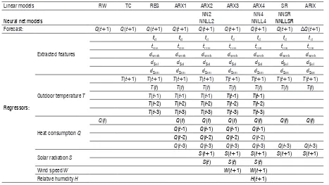
The following paragraphs describe the structures of examined forecasting models, and the list of regressors included in each model is summarized in Table 1.

3.1 Random Walk Model

The random walk (RW) model predictor Q(t+1) derives its value from past heat load Q(t), with e(t) denoting noise and t the arbitrary time in daily resolution:

Q t

(

)

( )

The random walk model is only considered as a basis to evaluate the other, more elaborate models, as recommended in [16] where RW model is implicitly included in the proposed mean absolute scaled error measure.

3.2 Temperature Correlation Model

The temperature correlation model (TC) correlates the heat load Q(t+1) with the average daily temperature T(t+1):

Q t

(

)

(

)

(

)

3.3 Regression Model

The linear regression model (REG) expands the selection of a single temperature input of a TC model in Eq. (3) by including also delayed temperature values T(t), T(t–1), …, and also informative features as described in Section 1.1. The list of included regressors is shown in Table 1.

3.4 Autoregressive Models

Autoregressive models (ARX) further expand the REG model by including as inputs as well as delayed heat load values Q(t), Q(t–1), … . Various applied ARX models differ only in the selection of additional weather-related inputs (see Table 1 for details).

The ARIX model has the same structure as the ARX model but forecasts the differences in daily heat load ΔQ instead of forecasting the absolute heat load Q.

3.5 Stepwise Regression Model

The stepwise regression model (SR) in this study is based on the initial selection of regressors provided by ARX models and is constructed by iteratively adding and removing regressors based on their statistical significance in a regression [17]. The method

begins with an initial model and then compares the explanatory power of incrementally larger and smaller models. At each step, the p-value of an F-statistic is computed in order to test models both with and without a potential input. Tested inputs are iteratively added or removed from the model until the procedure converges to a locally optimal forecasting model with statistically significant input variables. This method also resolves the collinearity problem by reducing the available set of inputs to the relevant ones.

3.6 Feedforward Neural Network

Feedforward neural network (NN) models [18] can be considered to be nonlinear auto-regressive models (NARX) that extend the ARX models with the ability to also encapsulate nonlinear system responses. In our study, a feedforward neural network with sigmoidal activation functions was applied, and the number of hidden neurons was kept low to prevent overfitting. For the same reason, the Levenberg-Marquardt learning algorithm with Bayesian regularization was applied to improve generalization.

The architecture of the NN with one hidden layer of neurons with sigmoidal activation function and a linear output layer is shown in Fig. 3. Based on the initial simulation results, the hidden layer consists of 5 hidden neurons. Increasing the number of hidden

Table 1. Summary of forecasting models and included regressors

Linear models RW TC REG ARX1 ARX2 ARX3 ARX4 SR ARIX

Neural net models

NN2 NNLL2

NN4 NNLL4

NNSR

NNLLSR

Forecast: Q(t+1) Q(t+1) Q(t+1) Q(t+1) Q(t+1) Q(t+1) Q(t+1) Q(t+1) ΔQ(t+1)

Regressors:

Extracted features

td td td td td td td

tcos tcos tcos tcos tcos tcos tcos

dwork dwork dwork dwork dwork dwork dwork

dSat dSat dSat dSat dSat dSat dSat

dSun dSun dSun dSun dSun dSun dSun

Outdoor temperature T

T(t+1) T(t+1) T(t+1) T(t+1) T(t+1) T(t+1) T(t+1) T(t+1)

T(t) T(t) T(t) T(t) T(t) T(t) T(t)

T(t-1) T(t-1) T(t-1) T(t-1) T(t-1)

T(t-2) T(t-2) T(t-2) T(t-2) T(t-2) T(t-3) T(t-3) T(t-3) T(t-3) T(t-3)

Heat consumption Q

Q(t) Q(t) Q(t) Q(t) Q(t) Q(t) Q(t)

Q(t-1) Q(t-1) Q(t-1) Q(t-1) Q(t-2) Q(t-2) Q(t-2) Q(t-2)

Q(t-3) Q(t-3) Q(t-3) Q(t-3) Q(t-3) Q(t-3)

Solar radiation S S(t+1) S(t+1) S(t+1) S(t+1) S(t+1) S(t) S(t) S(t)

Wind speed W W(t+1) W(t+1)

neurons did not improve the generalization ability of the model.

Fig. 3. Feedforward neural net (NN)

3.7 Feedforward NN with Direct Linear Link

In addition to the classic neural network architecture described above, an additional NN architecture with a direct linear link (NNLL) was applied due to the strong linear relationship between the input and output variables. The advantage of the NNLL architecture is its improved ability to directly model linear mappings with the additional capacity to add nonlinear responses. The NNLL architecture is presented in Fig. 4 where a direct linear link from the inputs to the output layer is shown. In this configuration, the hidden layer can be considered as a nonlinear feature extractor that provides additional features to the linear regression model implemented by a linear output layer. In our case study, only 2 nonlinear hidden layer neurons were used to prevent unnecessary overfitting.

Fig. 4. Feedforward neural net with direct linear link (NNLL)

The training procedure for all neural network models (NN and NNLL) included 200 repeated random initializations followed by gradient-based learning (until learning converged). The results reported include the average and the best result obtained from 200 training realizations.

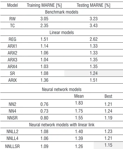
4 RESULTS

This section presents forecasting results obtained by applying the described forecasting models (Section 3) to the forecasting problem defined in Section 2. For all applied models both training and testing errors (MARNE) are presented, although only the testing error that is considered an estimator of the generalization ability of the model is evaluated as a

final model performance measure. Forecasting results for all models are summarized in Table 2.

It should be noted that applied linear models always converge to a unique solution, whereas nonlinear NN models converge only to locally optimal solutions depending on the initial conditions of free network parameters (synaptic weights of neurons) that form the basis for the subsequent gradient-based optimization. Consequently, the average results for multiple NN initializations are reported in Table 2 as well as the best obtained NN results. The best obtained testing results for linear and neural models are marked in gray.

Table 2. Forecasting results

Model Training MARNE [%] Testing MARNE [%] Benchmark models

RW 3.05 3.23

TC 2.35 3.43

Linear models

REG 1.51 2.62

ARX1 1.14 1.33

ARX2 1.06 1.33

ARX3 1.04 1.35

ARX4 1.03 1.35

SR 1.08 1.24

ARIX 1.36 1.51

Neural network models

Mean Best

NN2 0.76 1.83 1.21

NN4 0.73 1.75 1.24

NNSR 0.80 1.55 1.19

Neural network models with linear link NNLL2 1.08 1.40 1.23 NNLL4 1.06 1.39 1.21 NNLLSR 1.09 1.26 1.15

Both benchmark models (Table 2) yield initial generalization performance above 3 %: 3.23 % for the RW model and 3.43 % for the TC model. Although the training performance of TC model is better compared to RW model, its generalization performance is worse. A comparison of linear models reveals that the regression model (REG) considerably improves the initial performance of both benchmark models by reducing the training error to 1.51 % and the testing error to 2.62 %. This confirms the benefits of including the proposed extracted features and delayed terms of outdoor temperatures.

heat consumption as inputs. The results clearly demonstrate the importance of the autoregressive forecasting approach. ARX models that differ only in the inclusion of additional weather related inputs (S, W, H) show similar performance; therefore, it can be concluded that additional weather-related inputs only marginally contribute to forecasting performance.

Additional generalization improvement was obtained by applying the stepwise regression approach that reduces the available inputs to strictly relevant ones. In the case of a SR model, a training error of 1.08 % was obtained, and a testing error of 1.24 % which is the best result in the family of linear models. Beside the improved generalization ability, the SR model also reduces the model complexity and is therefore considered as an appropriate model for application in the district heating industry.

The application of the ARIX model that includes the integrating term and, therefore, forecasts the heat consumption difference ΔQ (instead of Q) did not improve the results.

The forecasting results obtained by NN-based models show the following various interesting conclusions:

• NN training depends on the initial (random) initialization of network parameters (weights) therefore multiple learning initializations followed by supervised gradient-based learning are required to ensure good NN performance. • Only a few hidden layer neurons are sufficient

to model this type of an energy consumption process.

• The best NN results generally achieve and exceed the same level as the best linear model, but the improvement is slight due to a very linear dependence Q(T).

• Due to the same reason of linear Q(T) dependence, NN with a direct linear link (NNLL) seems to be a good forecasting model, as demonstrated by testing results. The best NNLLSR model based on inputs selected by an SR model achieves testing performance of 1.15 % which is the overall best generalization result. In this case, only two hidden layer neurons with sigmoidal activation functions were used. These two neurons can be considered as additional automatic nonlinear feature extractors that are added to the linear model.

The best testing (generalization) results of applied models are compared in Fig. 5. It can be seen that NN based models slightly improve the performance of linear models. The best linear model (SR) yields a testing performance of 1.24 %, and the best NN-based model (NNLLSR) yields 1.15 % which represents a 7.3 % improvement in testing performance in comparison to the SR model.

Fig. 5. Testing results of linear and NN-based forecasting models

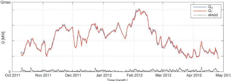
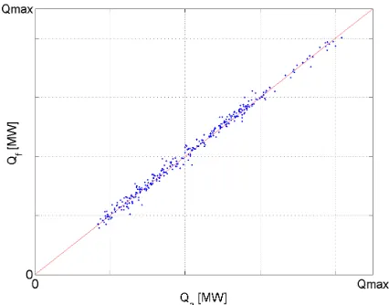
A graph of the forecasting results obtained by the best NNLLSR model is presented in Fig. 6. Actual heat consumption Qa, forecast heat consumption Qf, and absolute forecasting error e = abs(Qa – Qf) are shown for the selected test period from October 2011 to May 2012. The scatter plot of forecasting results (Qf vs. Qa) is shown in Fig. 7, where a very close matching can be observed (correlation coefficient R = 0.996).

Fig. 7. Scatter plot of all testing forecasting results (Qf vs. Qa)

5 CONCLUSIONS

A study of forecasting models for heat demand a day in advance in a district heating system is discussed in this paper. The study is based on district heating data for the city of Ljubljana, Slovenia, for five subsequent winter seasons. Additional weather related variables (temperature, solar radiation, wind speed, relative humidity) and extracted features (days of the week, linear trend, seasonal cycle) were applied in our forecasting approach. Various forecasting models, including simple benchmark models, linear regression and autoregressive models, and nonlinear neural network-based models were constructed for the forecasting task. The forecasting performance of the models was evaluated based on the generalization performance obtained by cross-validation on a test data set. The conclusions of this study can be summarized as follows:

• There is a strong linear relationship between the heat consumption Q and the outdoor temperature T. Consequently, the most significant regressor for the future heat load Q(t+1) forecasting is the outdoor temperature T(t+1).

• Other weather-related parameters are less important with the exception of solar radiation

S, which has been included as a significant regressor via a stepwise regression model. This is consistent with the results in the field of natural gas forecasting [19]. Wind speed and relative humidity do not have a significant impact on heat consumption.

• Heat consumption also exhibits autoregressive behaviour; therefore, including the past heat consumption {Q (t–k), k = 0, 1, …} into forecasting models considerably improves the forecasting accuracy.

• Due to a strong population influence on heat consumption, including additional extracted features denoting days of the week, linear trend and seasonal cycle, also significantly improves the forecasting accuracy.

• The best linear model for this forecasting task is the stepwise regression model (SR) that includes only significant regressors. This reduces the model complexity and also improves the generalization ability. Testing performance (expressed as a MARNE error) 1.24 % was obtained for the SR model.

• Comparison of linear and nonlinear forecasting models reveals that slight improvement is possible by applying properly trained nonlinear NN-based models. In the case of NN models, multiple weight initializations should be applied in order to converge network training toward solutions emphasizing good generalization ability.

interpreted to properly support control and business decisions. In our case study, the NNLLSR model improved the performance of a linear SR model by 7.3 %. This is a significant improvement that suggests that NN or the proposed NNLL structures are encouraged to be considered as forecasting solutions for applied forecasting in the district heating market. Further studies will be conducted to evaluate the adaptive versions of forecasting models [20], and take into account the influences of weather forecasting accuracy that influences heat load forecasts in online forecasting applications.

6 REFERENCES

[1] European Commission, Climate Action, Roadmap for moving to a low-carbon economy in 2050, from http://ec.europa.eu/ clima/ policies/roadmap/ accessed on 2015-02-26. [2] Connolly, D., Lund, H., Mathiesen, B.V., Werner, S., Möller, B.,

Persson, U., Boermans, T., Trier, D., Østergaard, P.A., Nielsen, S. (2014). Heat roadmap Europe: Combining district heating with heat savings to decarbonise the EU energy system. Energy Policy, vol. 65, p. 475-489, DOI:10.1016/j.enpol.2013.10.035. [3] Yeo, I.A., Yoon, S.H., Yee, J.J.: Development of an urban

demand forecasting system to support environmentally friendly urban planning. Applied Energy, vol. 110, p. 304-317,

DOI:10.1016/j.apenergy.2013.04.065.

[4] Soldo, B. (2012). Forecasting natural gas consumption. Applied Energy, vol. 92, p. 26-37, DOI:10.1016/j.

apenergy.2011.11.003.

[5] Mestekemper, T., Kauermann, G., Smith, M.S. (2013). A comparison of periodic autoregressive and dynamic factor models in intraday energy demand forecasting. International Journal of Forecasting, vol. 29, no. 1, p. 1-12, DOI:10.1016/j.

ijforecast.2012.03.003.

[6] Gadd, H., Werner, S. (2013). Daily heat load variations in Swedish district heating systems. Applied Energy, vol. 106, p. 47-55, DOI:10.1016/j.apenergy.2013.01.030.

[7] Dotzauer, E. (2002). Simple model for prediction of loads in district heating systems. Applied Energy, vol. 73, no. 3-4, p. 277–284, DOI:10.1016/S0306-2619(02)00078-8.

[8] Nielsen, H.A., Madsen, H. (2006). Modelling the heat consumption in district heating systems using a grey-box approach. Energy and Buildings, vol. 38, no. 1, p. 63-71,

DOI:10.1016/j.enbuild.2005.05.002.

[9] Lee, C.-M., Ko, C.-N. (2011). Short-term load forecasting using lifting scheme and ARIMA models. Expert Systems with Applications, vol. 38, p. 5902–5911, DOI:10.1016/j.

eswa.2010.11.033.

[10] Goia, A., May, C., Fusai, G. (2010). Functional clustering and

linear regression for peak load forecasting. International Journal of Forecasting, vol. 26, p. 700-711, DOI:10.1016/j.

ijforecast.2009.05.015.

[11] Aberg, M., Widén J. (2013). Development, validation and

application of a fixed district heating model structure that requires small amounts of input data. Energy Conversion and Management, vol. 75, p. 74-85, DOI:10.1016/j.

enconman.2013.05.032.

[12] Bacher, P., Madsen, H., Aalborg Nielsen, H., Perers, B. (2013).

Short-term heat load forecasting for single family houses.

Energy and buildings, vol. 65, p. 101-112, DOI:10.1016/j.

enbuild.2013.04.022.

[13] Thaler, M. (2009). An analytical-empirical model of heat

demand in a district heating system, PhD thesis. University of Ljubljana, Faculty of Mechanical Engineering, Ljubljana (in Slovene)

[14] Guo, Y., Nazarian, E., Ko, J., Rajurkar, K. (2014). Hourly cooling load forecasting using time-indexed ARX models with two-stage weighted least squares regression. Energy Conversion and Management, vol. 80, p. 46-53, DOI:10.1016/j.

enconman.2013.12.060.

[15] Powell, K.M., Sriprasad, A., Cole, W.J., Edgar, T.F. (2014). Heating, cooling, and electrical load forecasting for a large-scale district energy system. Energy, vol. 74, p. 877-885,

DOI:10.1016/j.energy.2014.07.064.

[16] Hyndman, R.J., Koehler, A.B. (2006). Another look at measures

of forecast accuracy. International Journal of Forecasting, vol. 22, no. 4, p. 679-688, DOI:10.1016/j.ijforecast.2006.03.001.

[17] Draper, N., Smith, H. (1981). Applied Regression Analysis, 2nd

ed. John Wiley & Sons, New York.

[18] Haykin, S. (2009). Neural Networks and Learning Machines,

3rd _{ed., Pearson, New York.}

[19] Soldo, B., Potočnik, P., Šimunović, G., Šarić, T., Govekar, E. (2014). Improving the residential natural gas consumption forecasting models by using solar radiation. Energy and Buildings, vol. 69, p. 498-506, DOI:10.1016/j.

enbuild.2013.11.032.

[20] Potočnik, P., Soldo, B., Šimunović, G., Šarić, T., Jeromen, A., Govekar, E. (2014). Comparison of static and adaptive models for short-term residential natural gas forecasting in Croatia. Applied Energy, vol. 129, p. 94-103, DOI:10.1016/j.