DEMOGRAPHIC RESEARCH
VOLUME 32, ARTICLE 2, PAGES 29
74
PUBLISHED 7 JANUARY 2015
http://www.demographic-research.org/Volumes/Vol32/2/ DOI: 10.4054/DemRes.2015.32.2
Research Article
Sibship size and height before, during, and after
the fertility decline:
A test of the resource dilution hypothesis
Stefan Öberg
©2015 Stefan Öberg.
This open-access work is published under the terms of the Creative Commons Attribution NonCommercial License 2.0 Germany, which permits use, reproduction & distribution in any medium for non-commercial purposes, provided the original author(s) and source are given credit.
1 Introduction 30
2 Previous research 31
3 Description of the data 35
4 Method 36
4.1 Theoretical model 37
4.2 Measuring sibship size 38
4.3 Model specifications 40
5 Context 43
6 Results 44
7 Discussion 50
8 Conclusions 54
9 Acknowledgements 54
References 55
Sibship size and height before, during, and after the fertility decline:
A test of the resource dilution hypothesis
Stefan Öberg1
Abstract
BACKGROUND
There is still much to learn about the explanation for the often-found negative association between sibship size and different child outcomes. A plausible explanation is resource competition between siblings in larger families, as suggested by the resource dilution hypothesis.
OBJECTIVE
This study contributes to our understanding of these mechanisms by investigating the association between sibship size and height before, during, and after the fertility decline to test predictions based on the resource dilution hypothesis.
METHODS
The investigation is conducted using information from universal conscript inspections linked to a longitudinal demographic database. Regression analyses estimate a model derived from the resource dilution explanation and analyze the association between sibship size and height among men born in 1821–1950 in southern Sweden.
RESULTS
The results show that the association between sibship size and height was negative from the mid-nineteenth century until the mid-twentieth century. There is no association in the early nineteenth century. The strength of the association is gradually weakened over time for men born from the 1840s until the 1940s. It is most consistent among men born from 1881–1921, corresponding closely to the time for the fertility decline in the area. The association is not a result of confounding by observable demographic or socioeconomic differences between families.
CONCLUSIONS
The results are in line with resource dilution being an important explanation for the negative association between sibship size and height. Resource dilution in larger families still seems to be dependent on the societal and historical context.
1. Introduction
A negative association between the number of children in a family, the sibship size, and the heights of the children has been shown many times for 20th century populations in high-income (Douglas and Simpson 1964; Olivier and Devigne 1983; Mednick et al. 1984; Lawson and Mace 2008; Suliga 2009) and low-income countries (Desai 1995; Jordan et al. 2012; Manley, Fernald, and Gertler 2012), even though no association has been found in some populations (Desai 1995). A negative association between sibship size and the children‟s outcomes has not only been observed with regard to height, but also, and in an even larger number of studies, with regard to the children‟s educational outcomes and social mobility (Blake 1981, 1985; Downey 1995, 2001; Sacerdote 2007; see also the review by Steelman et al. 2002).
The association between sibship size and child outcomes is thus firmly established, at least in 20th century high-income populations. Much less is known about the mechanisms that lead to these negative associations. The most-used explanations are resource dilution in larger families and confounding. The mechanisms behind the negative associations have implications for our understanding of family dynamics and behavior, and also for our understanding of the demographic transition (e.g., Becker 1993). The presence of the associations in historical populations also has implications for, for example, unified growth theory (Galor 2012) or the theory of the technophysio evolution (Floud et al. 2011). Both theories assume that resource dilution affects child outcomes and this is the most important (Galor 2012), or one of several (Floud et al. 2011), mechanism(s) generating dynamic effects in the models.
The fertility decline has also been proposed as an explanation for the secular increase in height and improving health of children from the late 19th century onwards (Reves 1985; Weir 1993; Schneider 1996; Hatton and Martin 2010a). Hatton and Martin (2010a), for example, retrospectively extrapolate based on cross-sectional data from 1930s Britain and suggest that about 25% of the increase in height should be attributed to the fertility decline. These suggestions also make it interesting to test how the association between the sibship size and the living conditions of children has developed longitudinally.
and landholding and has now been linked to heights from universal conscription inspections of men born in 1797–1950 (Öberg 2014a: Paper 5).
The long time period covered by the data used here makes it possible to test for differences in the association before, during, and after the fertility decline. If resource competition within families is an important explanation for the negative association between sibship size and child height, we should expect that the association is influenced by the average level of income. The resource dilution hypothesis therefore leads us to expect that the association between sibship size and child height has become more weakly negative over time. Other developments of the association than becoming more weakly negative over time require other explanations or that the behavior or social conditions of families have changed over time. More frequent or severe exposure to disease of children in larger families is one possible alternative or complementary explanation. While it is not possible to discriminate here between influences on growth and height from nutrition and disease it is not obvious that any negative influence from disease would become weaker over time. To the extent that disease exposure is influenced by housing quality and other preconditions for good hygiene, it is not separate from the resource dilution explanation.
The detailed longitudinal information in the SEDD also makes it possible to investigate the causes further by testing how much of the association can be explained by potential confounders. This provides excellent opportunities to test the resource dilution hypothesis through the following two research questions, addressed in this paper. Firstly, what was the association between sibship size and child height before, during, and after the fertility decline? Secondly, can the association be explained by confounding by observable differences between the families?
2. Previous research
The dilution of parental resources, and hence competition and resource scarcities in large families, is probably the most-used explanation for the negative association between sibship size and child outcomes, explicitly or implicitly (see e.g., Becker 1993). The resource dilution hypothesis has received a great deal of support in previous research (Downey 1995; Hertwig, Davis, and Sulloway 2002; Jæger 2009; Lawson and Mace 2009; Bras, Kok, and Mandemakers 2010; Lordan and Frijters 2013). If resource competition and scarcities within families, affecting nutrition and/or disease exposure, are important negative influences on heights in large families, we would expect the association to become weaker with rising real incomes (compare also e.g., Becker 1993: Ch. 6 and esp. 271).
Individual heights are largely determined by genetic and other biological factors, but are also, as mentioned, affected by environmental influences during childhood and adolescence. Negative environmental influences, such as suboptimal nutrition or disease, hinder individuals from reaching their genetic and biological height potential. When all the requirements and needs are met, more resources, for example nutritional, will have few positive influences on growth (Steckel 2008). Heights are consequently a better measure of resource deficiencies than of abundance. With rising real incomes we therefore also expect that children with many siblings will obtain enough resources to attain their height potential, even if resources are relatively scarcer in large families than in smaller ones. While desires for different kinds of consumption can change over time and thus change the meaning of limited resources alongside income levels (e.g., Alter 1992), human nutritional needs have not experienced any dramatic changes over the last 200 years. If resource dilution is an important explanation for the negative association between sibship size and child height, we can therefore safely expect rising real incomes to weaken the negative association.
The more or less explicit assumptions in the resource dilution hypothesis (as well as in e.g., Becker 1993) are that the limited and fixed resources provided by the parents are shared among all the children in the family without any economies or diseconomies of scale in the household production (for a discussion on the assumptions, see e.g., Desai 1995; Downey 2001 or Hertwig, Davis, and Sulloway 2002). If there are fundamental differences in the validity of any or several of these assumptions in different periods of time, then the association between family size and child heights could also change over time. Increasing costs of raising children and/or the costs of children falling increasingly on the biological parents could, for example, counteract the effect from a rising average level of income. Changing social patterns in living conditions and fertility behavior would also lead to the confounding of the association changing over time.
Hatton and Martin 2010a, 2010b; Kuh and Wadsworth 1989; Li, Manor, and Power 2004; Mascie-Taylor and Lasker 2005; Li, Dangour, and Power 2007) and Sweden (Cernerud 1993). There are some possible signs of a weakening of the association over the 20th century in both countries. Cernerud (1993) investigates the association among schoolchildren in Stockholm born in 1933, 1943, 1953, and 1963. He finds that the effect is about 20% weaker for the 1963 cohort than for the 1933 cohort. Li and Power (2004) find a similar decline when comparing the members of the British 1958 birth cohort with their offspring (born 1973–1987). Cernerud (1994) further finds no effect of the number of siblings on height among schoolchildren in Stockholm born in 1981. These results indicate a weakening of the relationship over time in these high-income populations, just as predicted if the association is caused by resource dilution.
Nothing is known about the association between sibship size and child height among those born before c.1930. If resource competition and scarcity are the causes, we would, as discussed, expect the association to be stronger in the 19th and the early 20th century than later. A few studies consider how the association between sibship size and other child outcomes, for example educational and social attainment, has changed over the very long run. Bras, Kok, and Mandemakers (2010) find that the negative effect of sibship size on chances for social status attainment in the Netherlands strengthened from the mid-19th to the early 20th century. Regarding social mobility, Van Bavel (2006) and Van Bavel et al. (2011) find negative effects of having many siblings during the fertility decline around 1900 in Belgium but do not investigate whether the effect changes over time. Studies on late 20th-century Indonesia (Maralani 2008), China (Lu and Treiman 2008), and Brazil (Marteleto and de Souza 2012) show that the relationship between sibship size and educational attainment has changed over time because of societal development and changing policies. The results of these studies are in line with the assumption that societal and economic changes can increase the parental costs of children over time and/or strengthen the confounding of the association.
An alternative explanation is, as mentioned, that families with many children are different from families with fewer in some observable or unobservable way that also affects the living conditions of the children. It could be, for example, that families with lower socioeconomic positions on average have more children than families with higher socioeconomic positions. The association between the number of children in the family and their living conditions is then confounded by the families‟ socioeconomic position and the number of children cannot be considered the (only) cause behind the association.
Previous studies have shown that confounding by observable or unobservable characteristics can be part of the explanation for the negative association between sibship size and child outcomes. Millimet and Wang (2011) find a negative effect on height from having more than one sibling in late 20th-century Indonesia, also when controlling for the possible endogeneity of the fertility choice. However, the effect is fully explained by differences between families in place of residence and parents‟ ages and level of education. The negative effect of family size on height in the 1958 British national birth cohort is also weakened a lot (the coefficients are weakened by more than 50%) when adjusting for parental heights and other controls (Li, Manor, and Power 2004; Li, Dangour, and Power 2007; see also the similar results in Lawson and Mace 2008 and Lordan and Frijters 2013). The relationship between the number of siblings and height in the 20th century thus seems to be interrelated with other family characteristics that more consistently influence height.
adjust for confounding while allowing the effect from the confounding variables to vary over time.
3. Description of the data
The data used come from the Scanian Economic Demographic Database (SEDD), which covers the population in five closely situated rural parishes in southern Sweden: Kävlinge, Hög, Kågeröd, Sireköpinge, and Halmstad (M) (Bengtsson, Dribe, and Svensson 2012). The database is a collaborative project between the Regional Archives in Lund and the Centre for Economic Demography at Lund University and has been underway since 1983 (Reuterswärd and Olsson 1993). All individuals born in or migrating into the included parishes are followed from birth or entry until death or out-migration. The database has been constructed from catechetical examination registers (husförhörslängder) and has been linked to tax registers (mantalslängder and
inkomstlängder) and checked against church books on births, marriages, migrations, and deaths (Dribe 2000). The data include all demographic events as well as information on occupations and landholding. Moves into and out of households are known from the catechetical examination registers. People moving into and marrying in the parishes before 1896 have been traced to their parish of origin to collect information on the socioeconomic status of the family at their birth.
Men born between 1797 and 1950, with a known family background and whereabouts around the time of conscription, have been traced in lists from universal conscript inspections (Öberg 2014a). About 80% of the men searched for in the lists were successfully linked. The populations in Kävlinge, Hög, and Kågeröd were included for the full time period. The creation of the longitudinal demographic database is highly labor intensive and time consuming. The data covering the populations in Sireköpinge or Halmstad (M) after 1895 were not yet completed when collecting the conscript data.
In this study we use a sub-sample of the conscripted men. The measure of sibship size used here is a time-weighted average of the number of children present in the family during the first ten years of the man‟s life. The men included in the sample therefore have to have lived for at least some part of their life from birth until the age of ten years in the database parishes. All the men included in the sample were born between 1821 and 1950 and were aged between 17 and 25 years at inspection. We only include men with mothers aged 17–50 years at their birth, to reduce the risk of errors in the data. The socioeconomic status of the head of household, usually the father, at the birth of the child is used for the socioeconomic variables. This reduces the difference in the information available for migrant and non-migrant families. Only men with information on the occupation and/or landholding of their family at their birth are included in the sample. Two men with heights below 140 centimeters have been excluded as potentially influential outliers. The final sample consists of 3,651 men from 2,322 families. The truncated regressions are in practice estimated using only the 3,320 observations (from 2,176 families) with information on height and for whom the height is above the minimum height requirement.
4. Method
As described above, there was a minimum height requirement in place during most of the 19th century. The height of men freed from conscription duty was not recorded in the lists until the latter part of the 19th century. For most of the 19th century, and especially among men born during the first half, there are therefore quite a few men with no information on their height in the inspection lists (Table 2). This led to a shortfall of heights at the lower end of the distribution (Öberg 2014b). Truncated regressions estimated using maximum likelihood were therefore used to account for this problem (Komlos 2004).2 Many of the men lacking information on their height were shorter than the minimum height requirement. The implicit assumption of the truncated regressions used is that all were shorter than the minimum height requirement. This is most likely not true but was deemed sufficiently accurate for using the truncated regressions.
The data hold different numbers of observations for different families. Large families and/or families with many sons can add more observations to the analyses. This is compensated for here by weighting the observations by the multiplicative inverse of the square root of the number of inspected sons in the family. For example, in
2 The truncation points used are 160.5 cm for men born 1813–1842, 160 cm for men born 1843–1865, and
the cases in which there are four men from the same family in the sample, each of the four brothers is down-weighted to add the equivalent of a one-half observation to the estimated regressions ( √ ⁄ ). We chose this, admittedly somewhat arbitrary, weighting as a compromise between not giving too much weight to families with many sons while still allowing for the fact that we do have more information on height for these families. All the standard errors are clustered at the family level to adjust for the expected correlations between brothers.
No attempts are made to adjust for the possible simultaneity or endogeneity bias caused by the parents‟ dynamic decisions on how many children to have and how much to invest in each. The point of the results is to determine whether there was an association and whether this varied over time, so it is not essential to have true estimates of causal relationships. The results should still be interpreted with the necessary caution.
4.1 Theoretical model
The resource dilution hypothesis leads to a non-linear functional form of the relationship between sibship size and child outcomes (Downey 1995, 2001). The amount of resources spent on each child, , is the family‟s total resources, , divided between the number of children, ; ⁄ . The negative effect of having many siblings should therefore be stronger for the first siblings added than for higher parities.3
The estimation of the relationship between the number of siblings and their heights here starts from the functional form expected from the resource dilution hypothesis. It then rests on the assumption that the relationship between the resources invested in the child, , and the child‟s height, , is log-linear. Diminishing returns in height to increases in family incomes or resources are in line with Becker‟s (1993) models, the theoretical expectations about environmental influences on growth (Steckel 2008), aggregate relationships between average height and level of income across countries (Baten and Blum 2012), and within most countries historically (Öberg 2014a: 24–26). Assuming a log-linear association between resources and height also has the crucial advantage of making it possible to estimate the model using linear regression, since it then turns out to be (see the Appendix for further discussion of the model):
The natural logarithm of the family income, , is approximated here with dummy variables indicating occupational status and landholding. From the derivation of
the model we should expect a negative value of the coefficient, , on the natural log of the number of children in the family, . A negative coefficient requires that differences in family income are adequately captured by the included variables and that the underlying assumptions of the resource dilution hypothesis are valid, e.g., that there are no strong economies of scale. and represent the family- and child-level control variables included in the estimations and and the family- and child-level residuals, respectively.
4.2 Measuring sibship size
The number of children in the family can be measured in a number of different ways; for example as the total number of children ever born in the family, the total number of surviving children (Van Bavel 2006; Van Bavel et al. 2011), or, as here, the time-weighted average of the number of children present in the household during each man‟s childhood (similar to Dribe 2000; Bengtsson 2009; Kippen and Walters 2012). Different measures do not necessarily produce the same results for the association between sibship size and child outcomes (Kippen and Walters 2012). The measure used here was judged to be best in line with the resource dilution hypothesis. The time-weighted average used here is calculated using the continuous information and is the cumulative sibship size exposure until age ten. We count the number of children present in the household for each time period of observation from a man‟s birth or first appearance in the database parishes until his tenth birthday. The measure includes the observed man himself, so that a man without siblings has a sibship size of one. A man with one sibling present from his birth until the age of ten, for example, obtains a value of 2 (himself + his sibling). The number of children present is not counted only in full integers, so if another child had been born at the man‟s exact age of five years, he would have received the value 2.5. Siblings dying are counted while present in the household, but not afterwards.
height and birth order was negative among men in Sweden born later during the 20th century (1965–1978).
We include the birth order of the men in the estimated models. The birth order is counted as births to a specific mother and all known, including deceased, siblings are included in the measure of birth order. Children not observed at birth but only, for example, living with a mother when moving into the database parishes are included in the birth order (as well as the sibship size measures). Births occurring outside the covered parishes and for which the child died before the move into the observed population are not included. Births occurring after leaving the parishes are also omitted. There is therefore some miscounting of the total number of births and children present. The birth order should still reflect whether the child is born early or late among the children included in the calculations of the sibship size variable. Summary statistics of the sibship size variable and other measures of family configuration are presented in Table 1.
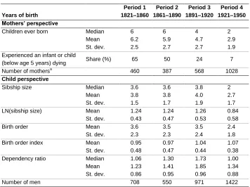
Table 1: Summary statistics of family configuration
Period 1 Period 2 Period 3 Period 4
Years of birth 1821–1860 1861–1890 1891–1920 1921–1950
Mothers’ perspective
Children ever born Median
Mean St. dev. 6 6.2 2.5 6 5.9 2.7 4 4.7 2.7 2 2.9 1.9 Experienced an infant or child
(below age 5 years) dying Share (%) 65 50 24 7
Number of mothersa 460 387 568 1028
Child perspective
Sibship size Median
Mean St. dev. 3.6 3.8 1.5 3.6 3.8 1.7 3.8 4.0 1.9 2 2.7 1.7
LN(sibship size) Mean
St. dev. 1.24 0.43 1.24 0.47 1.26 0.53 0.84 0.58
Birth order Mean
St. dev. 3.6 2.3 3.5 2.3 3.5 2.4 2.4 1.8
Birth order index Mean
St. dev. 0.95 0.48 0.97 0.47 1.04 0.44 1.07 0.38
Dependency ratio Median
Mean St. dev. 1.06 1.23 0.86 1.30 1.41 0.95 1.73 1.85 0.96 1.00 1.34 0.88
Number of men 708 550 971 1422
a
Birth order is quite naturally highly correlated with the number of children present in the household (r = 0.73). The number of children present will tend to be higher for the men born as middle children. The measure of sibship size used here captures this variation. The additional control for birth order is intended to capture any systematic differences in height between children born early or late in the sibship. Since the birth order and the sibship size are highly correlated, it is not possible to include both measures in the estimated models as they are. We therefore use the birth order index proposed by Booth and Kee (2009).4 The index is a measure of relative birth order standardized so that the average is equal to 1 in all the families and in the population. The index is still positively correlated with the sibship size (r = 0.30, r = 0.32–0.41 within the sub-periods used in the analyses) but can now be entered into the regression models without causing problems of multicollinearity. A resource dilution framework should lead us to expect a non-linear association between the birth order and the family resources available per child (Hertwig, Davis, and Sulloway 2002). The birth order index is therefore included both as a linear and as a quadratic term.
4.3 Model specifications
The regression models used here to test the influence on height of the number of children in the family are in line with that proposed by Van Bavel (2006). They are what Van Bavel calls “child perspective models”, since they also control for child-specific characteristics such as birth order. The models deviate from Van Bavel‟s in the measure used for sibship size.
Three different models are estimated. The first, Model A, includes the natural logarithm of the number of children present in the household during the first ten years of the men‟s lives and birth order along with individual-level control variables. The included controls are the decade of birth, age at inspection5, whether the man volunteered for conscription before the compulsory age or was a hired recruit, and an indicator of whether the man was not living in the database parishes during all the years from birth until the age of ten years.
Model B includes the variables in Model A along with other demographic controls: an indicator of families with only one observed child and an indicator of whether the mother or father in the family died before the age of 50 years. It is possible that the
4 The birth order index is the sibship-size standardized relative birth order and is calculated using the formula: (( ) ⁄ ⁄ ) (Booth and Kee 2009: 378f). The within-family and overall average is 1, with lower values for early born children and high values for later-born children. The range of values in the data analyzed here is 0.133 to 1.857.
5
single birth was a result of these families being disadvantaged through, for example, a worse health status of the parents. This group always constitutes a small minority of the families, at least during the 19th and the early 20th century (Table 2), but might influence the estimates of the association between sibship size and child height. Families in which a parent died prematurely can be expected to have fewer children, while the children can also be expected to have had worse living conditions growing up. The included indicator should control for this variation.
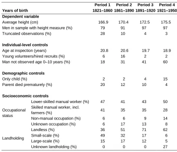
Table 2: Summary statistics of the dependent variable and control variables
Period 1 Period 2 Period 3 Period 4
Years of birth 1821–1860 1861–1890 1891–1920 1921–1950
Dependent variable
Average height (cm) 166.9 170.4 172.5 175.5
Men in sample with height measure (%) 79 91 97 97
Truncated observations (%) 28 10 4 3
Individual-level controls
Age at inspection (years) 20.8 20.6 19.7 18.9
Young volunteers/hired recruits (%) 6 16 2 2
Man not observed age 0–10 years (%) 18 31 41 60
Demographic controls
Only child (%) 2 2 4 15
Parent died prematurely (%) 20 12 10 4
Socioeconomic controls
Occupational status
Lower-skilled manual worker (%) 47 41 43 50
Skilled manual worker, incl.
farmers (%) 41 35 35 28
Non-manual occupation (%) 6 6 9 14
Unknown occupation (%) 6 17 13 8
Landholding
Landless (%) 36 51 71 62
Small-scale (%) 49 32 17 6
Large-scale (%) 15 17 12 5
Unknown landholding (%) 0 0 0 27
information from before the man‟s fifth birthday is used. The occupational status is based on the historical occupational class scheme HISCLASS (van Leeuwen and Maas 2011). Only three groups are separated: lower-skilled manual workers (HISCLASS 9–12), skilled manual workers (including farmers, HISCLASS 6–8), and non-manual workers (HISCLASS 1–5). Landholding is also separated into three categories: landless (including unknown) and small- and large-scale landholding. Missing information on occupation or landholding is included as separate categories. For further discussions on the socioeconomic indicators, see Öberg (2014a: Introduction, 2014b).
When estimating associations over long periods of time it is important to allow the effect of control variables to change over time. All the controls here were allowed to have different effects in the different time periods. This is achieved by interacting all included variables with indicators for three periods, excluding the fourth, latest period as the reference category. All effect estimates presented for periods other than the reference period, Period 4, are combined coefficients found by adding coefficients.
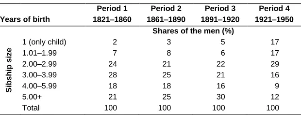
Only model C estimates the association as set out in the formal model specification, since this requires controls for the family‟s available resources. Only the coefficients for the sibship size variable are presented in Table 4. The controls are not presented in the paper since they are only included to estimate the formal model and to investigate the amount of confounding (the full results are available in the Appendix). Table 2 presents summary statistics for the control variables, except the variables describing the family configurations, which are shown in Table 1. Table 3 shows how the distribution of sibship size developed over time.
Table 3: The distribution of different sibship sizes among the men
Period 1 Period 2 Period 3 Period 4
Years of birth 1821–1860 1861–1890 1891–1920 1921–1950
Shares of the men (%)
S
ibsh
ip
s
iz
e
1 (only child) 2 3 5 17
1.01–1.99 7 8 6 17
2.00–2.99 24 21 22 29
3.00–3.99 28 25 21 16
4.00–5.99 18 18 16 9
5.00+ 21 25 30 12
Total 100 100 100 100
around 1890 in Scania, at approximately the same time as in the rest of Sweden (Bengtsson and Dribe 2014). There were some differences in behavior between older and younger mothers, but overall there was a strong period effect in the fertility decline in Sweden (Stanfors 2003; Dribe 2009; Bengtsson and Dribe 2014). The men in the studied sample are therefore divided into groups based on their years of birth: Period 1: 1821–1860; Period 2: 1861–1890; Period 3: 1891–1920; and Period 4: 1921–1950. The first and second periods correspond to the pre-transition era. The third period covers the early and the fourth the late/post-transition period. The fourth time period is used as the reference since it provides sizeable numbers of observations for all the categories.
To further investigate the change of the association over time we also estimate a „rolling regression‟. In this case this is 111 regressions, each estimated to include men born within a moving 20-year period. In this way we can see how the coefficient on sibship size changes over time in more detail than in the coarser periodization. The results are presented graphically in Figure 3. The estimated model is the same as Model C, except that the control for decade of birth is specified as an indicator for the later 10 years of birth included in each sample.
5. Context
The average height of conscripts increased almost linearly over time among men in the SEDD starting with cohorts born after the 1820s (Öberg 2014b: Figure 1). The secular trend in heights in the SEDD data is similar to the trend in Sweden in general. Both the secular trend in height and the long-term trend in real wages (Lundh 2008) show improving conditions in southern Sweden at least from the mid-19th century. Before the fertility decline the average mother had about 6 children and the average child about 2.5 siblings present in the household during childhood (Table 1). The average number of children ever born to a mother declined clearly in the third and fourth periods to about 2 children in the last period. This illustrates well the fertility decline in the SEDD population previously described by Bengtsson and Dribe (2014). Despite this the average number of children present in the household is stable from the early 19th to the early 20th century. This is probably, at least partly, a result of the falling infant and child mortality that can be followed in the drastically declining share of the families experiencing any deaths (Table 1). Most families (65%) experienced an infant or child dying in the early 19th century but the share fell for each time period, reaching a low 7% in the mid-20th century.6 Another possible explanation for the rising number of children present is that the children remained for longer in their parents‟ household over
6
time. The number of children present in the household changed only in the fourth period, among men born from 1920 onwards (Tables 1 and 3). In the fourth, late/post-transitional period, the distribution is clearly different from that in the preceding periods.
6. Results
The regression results show that sibship size is negatively associated with height in all the time periods and all the specifications (Table 4). In Model A, with only individual-level controls, the coefficient varies in strength over time and is most strongly negative and statistically significant in the third period. Adding the controls for single child families and parents dying prematurely brings out a stronger negative association in all time periods (Model B).
Table 4: Change in the association between sibship size and early adult height over time
Dependent variable:
height Year of birth
Period 1 Period 2 Period 3 Period4
1821–1860 1861–1890 1891–1920 1921–1950
Model A. Individual level variables
LN(sibship size) Coeff.
(s.e.) ‒0.7 (0.97) ‒0.6 (0.80) ‒0.8* (0.49) ‒0.5 (0.39)
Model B. Model A + other demographic controls
LN(sibship size) Coeff.
(s.e.) ‒0.8 (1.06) ‒1.1 (0.85) ‒1.2** (0.55) ‒0.8* (0.47)
Model C. Model B + controls of socioeconomic status (theoretical resource dilution model)
LN(sibship size) Coeff.
(s.e.) ‒1.3 (1.03) ‒1.2 (0.87) ‒1.3** (0.54) ‒0.7 (0.47)
Note: Single (Period 4) and combined coefficients (Periods 1–3) from truncated regressions estimating the association between the natural logarithm of the time-weighted average number of children present in the household and the early adult height. Standard errors clustered at the family level are shown within parentheses below the coefficients of interest. The complete regression results are available in the Appendix. Statistical significance of the single or combined coefficients are indicated as: * p<0.10, ** p<0.05, *** p<0.01.
others. The coefficients are again sizeable (between ‒0.4 and ‒1.6 cm) but only statistically significant in the third period (results in the Appendix). The negative effect of a parental death increases in strength over the 19th century and is strongest in the third period (men born 1891–1920).
Model C is the first to estimate the theoretical model set out in Section 4.1, since this includes controls for the resources available to the family. The negative coefficients for the first three time periods are very similar across periods and vary between ‒1.2 and ‒1.3. The corresponding height penalty between men growing up with different numbers of siblings present in the household during childhood increases with the number of siblings but with diminishing strength ( ; 1 sibling: ‒0.9 cm, 2 siblings: ‒1.4 cm, 3 siblings: ‒1.8 cm, 4 siblings: ‒2.1 cm, 5 siblings: ‒2.3 cm).
Model C includes a control variable for single children. Even if the coefficient never reaches statistical significance it should be remembered that the association between sibship size and height is both non-linear and includes a negative shift for single children. Single children were on average of about the same height as children with two or more siblings. The height differences were therefore in practice small. The purpose of the present study is not to explain the within-population variation in height but to investigate if resource dilution within larger families resulted in shorter stature of the children. That early adult height indeed was negatively associated with sibship size is, as discussed above, a strong indication of resource dilution in larger families.
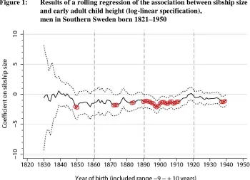
The estimated coefficient on sibship size from Model C is almost constant across the first three periods until the last late/post-transition period. This is not what we would expect if resource dilution were an important explanation of the association. The periodization used for these regressions is coarse and could conceal considerable variation. We therefore investigated the change of the association over time using rolling regressions (Figure 1).
The results from the rolling regression do indeed qualify the results. The graph shows that the periodization used for the results above conceal how the association changed over time. There are three dominating patterns: firstly, the lack of a negative association in the early 19th century; secondly, the long-term decline of the strength of the negative association from the mid-19th century until the mid-20th century; and thirdly, that the association is statistically significant primarily between the late 1880s and early 1910s.
Figure 1: Results of a rolling regression of the association between sibship size and early adult child height (log-linear specification),
men in Southern Sweden born 1821–1950
Note: The vertical dashed lines indicate the limits for the periodization used in the paper. The regressions underlying this figure each included men born during a 20 years period. In the figure the results are shown for the year in the middle of the range. The variables included are the same as for Model C. The only difference was that decade of birth was controlled for by an indicator variable unique for each sample for the men born during the ten later included years.
The association is only steadily statistically significant among men born between 1881 and 1921 (coefficients reported for 1890–1911). The association is statistically significant also in other years but only for three years in a row at most. The coefficients are only statistically significant at a 10% level, so we should be open to the possibility that one out of ten estimates is statistically significant by chance alone. The period when the association is statistically significant corresponds approximately to period three when we found the statistically significant results also in Model C in Table 4. Each period covered by the rolling regression is shorter than the static periods. The sample size in each of the samples analyzed for the rolling regression is therefore smaller than the ones used for the regressions reported in Table 4. This can contribute to the lack of statistical significance in some cases, especially in the early and mid-19th century, but the association does seem to have been most consistent among men born between 1881 and 1921.
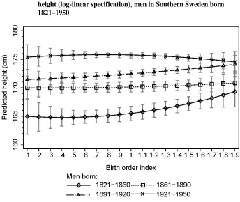
Controlling for birth order does not much change the estimated association between sibship size and height. This is in line with previous studies that likewise find that the negative association between sibship size and height remains after controlling for birth order (Belmont, Stein, and Susser 1975; Olivier and Devigne 1983; Li and Power 2004). The association between birth order and height is never statistically significant. It is weakly positive in the first and third periods, so that later-born sons are somewhat taller than earlier-born sons (Figure 2).
Figure 2: The association between birth order (index) and early adult child height (log-linear specification), men in Southern Sweden born 1821–1950
Figure 3: The association between sibship size and early adult child height (quadratic specification), men in Southern Sweden born 1821–1950
Note: The figure was produced using the margins and marginsplot commands in Stata 13.1.
We also checked if the miscounting of sibship size influences the results by repeating the analyses while including only the men that are fully observed for all the first ten years after birth. The results are again very similar but with stronger negative coefficients in the first three periods but a weakly positive coefficient in the last (results in the Appendix). The miscounting for men that are not fully observed therefore seems to reduce the strength of the association just as we would expect from measurement error. The true coefficient is likely to be more strongly negative than the ones reported in Table 4 and Figures 1 and 3.
child death but not all families, even among those with many children (Table 1). The coefficient on this variable is weakly positive (between +0.4 and +0.7) in the first three periods and weakly negative (‒0.2) in the last, but is never statistically significant. Including this variable also does not change the estimated association between sibship size and height (results in the Appendix). We cannot exclude that exposure to disease was part of the underlying causes of the negative association based on this. Repeated, non-lethal disease, especially gastrointestinal disease, can reduce growth and might have been part of the explanation (Stephensen 1999; Hatton and Martin 2010a).
7. Discussion
Estimating the theoretical resource dilution model while also controlling for possible confounders (Model C) results in a sizeable negative association between sibship size and early adult height during the 19thand the early 20th century. The presence and the negative sign of the coefficient are in line with a resource dilution explanation of the association.
The estimated associations are overall strongly influenced by observable differences between the families. The importance of confounding does not contradict the resource dilution hypothesis, since for the first three periods the negative associations between sibship size and height are rather concealed than generated by confounding by the demographic and socioeconomic differences between the families.7 By contrast, the association seems to be somewhat strengthened by confounding in the last period. The confounding of the association hence changed over time.
The change in the confounding from socioeconomic status comes about because there were socioeconomic differences in height (Öberg 2014b), family size (Table 5), and also in the timing of the fertility decline (Bengtsson and Dribe 2014). All other socioeconomic groups had on average more children present in the household than fathers with lower-skilled manual occupations in the first period (Table 5). In the second period it is only fathers with skilled manual or non-manual occupations that have more children present than others. But the elite, and also to some degree middle class, families limited their fertility before the lower-status groups. By contrast, landholding families remained larger than others throughout the studied time period. Sons from better-positioned families, especially with regard to the father‟s occupation, also remained taller also in the latter time periods but now lived on average in smaller
7 Preliminary analyses showed that it was very important to allow the effect of the confounders to vary over
families. Controlling for socioeconomic status therefore slightly weakens the negative association between sibship size and height in the late/post-fertility transition period.
Table 5: Socioeconomic differences in the number of children present during the men’s childhoods
Socioeconomic background
Period 1 Period 2 Period 3 Period 4
Year of birth 1821–1860 1861–1890 1891–1920 1921–1950
Number of children present Landless, lower-skilled
manual workers (ref.) 3.2 3.5 3.9 2.9
Skilled manual workers +0.4 *** +0.6 *** ‒0.1 ‒0.3 **
Non-manual occupations +1.2 *** +1.0 * ‒0.5 ‒0.5 ***
Unknown occupation +0.8 ** +0.2 ‒0.4 ** +0.3 *
Small-scale landholding +0.4 *** +0.1 +0.4 * +0.7 **
Large-scale landholding +0.5 * +0.1 +1.2 *** +0.7 ***
Unknown landholding — — — ‒0.3 **
R2 0.144
Number of observations 708 550 971 1422
Note: Table 5 shows the results from an ordinary least squares regression estimating the differences in the time-weighted average number of children present in the household during each man’s childhood (0–10 years) related to the socioeconomic status of the father. Statistical significance of the single or combined coefficients are indicated as: * p<0.10, ** p<0.05, *** p<0.01.
The results from the rolling regression show a clear, gradual, and statistically significant weakening of the association among men born from the 1840s onwards. The secular trend in height started in the studied area among men born in the 1830s (Öberg 2014b); real wages started to increase from the mid-19th century (Lundh 2008). This change of the association over time is therefore almost exactly what we would expect if resource dilution were an important factor causing the association. The weak negative association between sibship size and height in the mid-20th century is also in line with a recent study investigating this issue among Swedish conscripted men born in 1965– 1978 (Lundborg, Ralsmark, and Rooth 2013).
large families. The combination of rising expectations of what should be provided for the children (e.g., Alter 1992) in combination with rising sibship sizes could have worsened this resource scarcity around the time of the fertility decline. Another possible explanation of the pattern is that families that were better endowed in some unobserved way both created a more favorable environment for their children and limited their fertility earlier. Both explanations of the pattern are interesting for our understanding of the fertility decline, but unfortunately we are not able to examine them explicitly here.
The persistently negative association between sibship size and height also makes it possible that resource competition within families contributed somewhat to the shorter stature during the 19thand early 20th century. The reduced resource dilution after the fertility decline could therefore have contributed to the increasing heights in the present population. The change of the average sibship size (natural logarithm of sibship size from 1.26 to 0.84) from the third to the fourth period could have contributed to a c.0.5cm change (‒1.3×[1.26‒0.84]), out of the c.3cm change in average height over the same period. The possible contribution is therefore less than 20% but the magnitude of the effect is similar, if somewhat smaller, to the one reported in Hatton and Martin (2010a).
The estimated coefficient for the earliest years covered is, unexpectedly, weakly negative (Figure 1). There are several possible explanations for this. The weak association could be a result of the fact that, even if resource dilution in larger families is an important part of the explanation of the negative association between sibship size and height, changes in the societal context also influenced the association. Social and societal conditions in the early 19th century might have been less in line with the assumptions underlying the resource dilution hypothesis. The three assumptions are, as discussed above, that: i) all the income or resources come from the parents; ii) the parents do not adjust their income or own consumption when they have more children; and iii) there are no economies or diseconomies of scale in the household production.
children. The share of men missing information on height in the inspection lists and the large share of observations below the truncation points also lead to the coefficient being estimated with less precision. The weaker coefficient in the early and mid-19thcentury does not necessarily contradict the resource dilution explanation, but indicates that the social context might have been important for the association.
While the negative association points to resource scarcity in large families we cannot conclude much from the results with regard to the underlying proximate causes. Previous research shows that most likely there are also several different proximate causes behind the association between sibship size and child height within a resource dilution framework. Whitley and coauthors (2008) also find a negative association between sibship size and child height in 1930s‟ Britain also when controlling for household energy consumption and diet. Cernerud (1993) finds that the negative association remains among mid-20th-century schoolchildren in Stockholm, Sweden, after controlling for crowding in the home. The results of Hatton and Martin (2010a), analyzing the same data set as Whitley et al. (2008), support the supposition that familial resources were important for the negative association between sibship size and child health and height. They conclude that both nutrition, from family resources spent on food, and disease, working through housing quality and hygiene, contributed to generating the negative associations. Another possible contributing factor is child and adolescent work. In Brazil in the early 1990s an increasing number of children in the family decreased school attendance and increased the labor force participation of boys and girls and the share of girls having household chores as their main activity (Ponczek and de Souza 2012).
In Sweden in the early 20th century there were differences in diet between large and small families that could have contributed to differences in height. The Swedish Ministry of Health and Social Affairs carried out an official investigation into the living conditions and food consumption of families in the early 1940s (Socialdepartementet 1946: 117–139). They found that the absolute amount of money and the share of income spent on food quite naturally increased with the number of children in the family. However, families with many children spent less per consuming unit8 on food (see also Logan 2011). Large families still kept their energy consumption on a level similar to that of other families, but their diet was of a lower quality, more monotonous, and focused on cheaper foodstuffs. They consumed more milk, margarine, potatoes, and flour but less butter, meat, eggs, fish, and vegetables. The cheaper, less varied, diets were still very similar across family sizes with regard to macronutrients (compare also Lundh 2013). However, since children require relatively more protein for growing than adults, it is still possible that the diets in the larger families were inadequate. The on average adequate, with regards to macronutrients and energy consumption, diet also
8
concealed variation, with some families consuming inadequate diets. The diets of large families also often meant insufficient intakes of, for example, iron and vitamins A and B. If the dietary differences revealed by the Social Board in the early 1940s were also valid previously, these differences could be part of the explanation for the differences in height.
The association between birth order and height changes over time, but is never strong or statistically significant. The strongest pattern found is the positive association in the first, early and mid-19th century period (compare Alter and Oris 2008). This could be the result of resource accumulation in the families making a relatively larger positive contribution to the living conditions of the children in the generally poorer families during the nineteenth century than later.
8. Conclusions
We find a negative association between sibship size and height, thus indicating resource scarcity in large families. The results are in line with the assertion that resource dilution is an important explanation of the negative association between sibship size and child height. This association gradually weakened from the 1840s until the 1940s. The association was most consistent and therefore statistically significant during the fertility decline. The development of the association over time is generally as predicted by a resource dilution explanation. The association is, surprisingly, weakly negative in the early 19thcentury, but there are several potential explanations for this; for example, the household strategies used to balance the dependency ratio and the socioeconomic differences in fertility during this period. Confounding influences the estimated association, but in the present population mostly works to mask the negative association between sibship size and height during the 19thand the early 20th centuries.
9. Acknowledgements
The author would like to express his gratitude towards the Centre for Economic Demography, Lund University, for its collaboration and support. I thank the editors of
References
Alberman, E., Filakti, H., Williams, S., Evans, S.J.W., and Emanuel, I. (1991). Early influences on the secular change in adult height between the parents and children of the 1958 birth cohort. Annals of Human Biology 18(2): 127–136. doi:10.1080/03014469100001472.
Alter, G. (1992). Theories of Fertility Decline: A Nonspecialist‟s Guide to the Current Debate. In: Gillis, J.R., Tilly, L.A. and Levine, D. (eds.). The European Experience of Declining Fertility, 1850‒1970. Cambridge & Oxford: Blackwell: 13‒27.
Alter, G. and Oris, M. (2008). Effects of inheritance and environment on the heights of brothers in 19th-century Belgium. Human Nature 19(1): 44–55. doi:10.1007/ s12110-008-9029-1.
Ariès, P. (1980). Two successive motivations for the declining birth rate in the west.
Population and Development Review 6(4): 645–650. doi:10.2307/1972930. Baten, J. and Blum, M. (2012). Growing tall but unequal: New findings and new
background evidence on anthropometric welfare in 156 countries, 1810–1989.
Economic History of Developing Regions 27(1): 66–85. doi:10.1080/2078038 9.2012.657489.
Becker, G.S. (1993). A Treatise on the Family. Cambridge: Harvard University Press. Belmont, L., Stein, Z.A., and Susser, M.W. (1975). Comparison of associations of birth
order with intelligence test score and height. Nature 255(5503): 54–56. doi:10.1038/255054a0.
Bengtsson, T. (2009). Mortality and social class in four Scanian parishes, 1766–1865. In: Bengtsson,T., Campbell, C., Lee, J.Z. et al. (eds.). Life under pressure. Mortality and living standards in Europe and Asia, 1700–1900. Cambridge & London: The MIT Press: 135–171.
Bengtsson, T., and Dribe, M. (2014). The Historical Fertility Transition at the Micro Level: Southern Sweden 1815-1939. Demographic Research 30(17): 493–534. doi:10.4054/DemRes.2014.30.17.
Blake, J. (1981). Family size and the quality of children. Demography 18(4): 421–442. doi:10.2307/2060941.
Blake, J. (1985). Number of siblings and educational mobility. American Sociological Review 50(1): 84–94. doi:10.2307/2095342.
Booth, A.L. and Kee, H.J. (2009). Birth order matters: The effect of family size and birth order on educational attainment. Journal of Population Economics 22(2): 367–397. doi:10.1007/s00148-007-0181-4.
Bras, H., Kok, J., and Mandemakers, K. (2010). Sibship size and status attainment across contexts: Evidence from the Netherlands, 1840–1925. Demographic Research 23(4): 73–104. doi:10.4054/DemRes.2010.23.4.
Caldwell, J.C. (1976). Toward a restatement of demographic transition theory.
Population and Development Review 2(3/4): 321–366. doi:10.2307/1971615. Caldwell, J.C. (2005). On net intergenerational wealth flows: An update. Population
and Development Review 31(4): 721–740. doi:10.1111/j.1728-4457.2005. 00095.x.
Cernerud, L. (1993). The association between height and some structural social variables: A study of 10-year-old children in Stockholm during 40 years. Annals of Human Biology 20(5): 469–476. doi:10.1080/03014469300002862.
Cernerud, L. (1994). Are there still social inequalities in height and body mass index of Stockholm children? Scandinavian Journal of Social Medicine 22(3): 161–165. Desai, S. (1995). When are children from large families disadvantaged? Evidence from
cross-national analyses. Population Studies 49(2): 195–210. doi:10.1080/ 0032472031000148466.
Douglas, J.W.B. and Simpson, H.R. (1964). Height in relation to puberty, family size and social class: A longitudinal study. The Milbank Memorial Fund Quarterly
42(3): 20–34. doi:10.2307/3348625.
Downey, D.B. (1995). When bigger is not better: Family size, parental resources, and children‟s educational performance. American Sociological Review 60(5): 746. doi:10.2307/2096320.
Dribe, M. (2000). Leaving home in a peasant society: Economic fluctuations, household dynamics and youth migration in Southern Sweden, 1829–1866. [PhD Thesis]. Lund: Lund University, Lund Studies in Economic History.
Dribe, M. (2009). Demand and supply factors in the fertility transition: A county-level analysis of age-specific marital fertility in Sweden, 1880–1930. European Review of Economic History 13(1): 65–94. doi:10.1017/S1361491608002372. Eveleth, P.B. and Tanner, J.M. (1990). Worldwide variation in human growth.
Cambridge: Cambridge University Press.
Fernihough, A. (2011). Human capital and the quantity–quality trade-off during the demographic transition. UCD Centre for Economic. Dublin: School of Economics, University College Dublin (WP11/13).
Floud, R., Fogel, R.W., Harris, B., and Hong, S.C. (2011). The changing body: Health, nutrition, and human development in the western world since 1700. Cambridge: Cambridge University Press. doi:10.1017/CBO9780511975912.
Galor, O. (2012). The demographic transition: Causes and consequences. Cliometrica
6(1): 1–28. doi:10.1007/s11698-011-0062-7.
Gipson, J.D., Koenig, M.A., and Hindin, M.J. (2008). The effects of unintended pregnancy on infant, child, and parental health: A review of the literature.
Studies in Family Planning 39(1): 18–38. doi:10.1111/j.1728-4465.2008. 00148.x.
Hatton, T.J. and Martin, R.M. (2010a). Fertility decline and the heights of children in Britain, 1886–1938. Explorations in Economic History 47(4): 505–519. doi:10.1016/j.eeh.2010.05.003.
Hatton, T.J. and Martin, R.M. (2010b). The effects on stature of poverty, family size, and birth order: British children in the 1930s. Oxford Economic Papers – New Series 62(1): 157–184.
Hertwig, R., Davis, J.N., and Sulloway, F.J. (2002). Parental investment: How an equity motive can produce inequality. Psychological Bulletin 128(5): 728–745. doi:10.1037/0033-2909.128.5.728.
Jordan, S., Lim, L., Seubsman, S., Bain, C., Sleigh, A., and Thai Cohort Study Team. (2012). Secular Changes and Predictors of Adult Height Amongst Thai Cohort Study Participants Born 1940-1990. Journal of Epidemiology and Community Health 66(1): 75–80. doi:10.1136/jech.2010.113043.
Kippen, R. and Walters, S. (2012). Is sibling rivalry fatal? Siblings and mortality clustering. Journal of Interdisciplinary History 42(4): 571–591. doi:10.1162/ JINH_a_00305.
Komlos, J. (2004). How to (and how not to) analyze deficient height samples.
Historical Methods 37(4): 160–173. doi:10.3200/HMTS.37.4.160-173.
Kuh, D. and Wadsworth, M. (1989). Parental height – Childhood environment and subsequent adult height in a national birth cohort. International Journal of Epidemiology 18(3): 663–668. doi:10.1093/ije/18.3.663.
Lawson, D.W. and Mace, R. (2008). Sibling configuration and childhood growth in contemporary British families. International Journal of Epidemiology 37(6): 1408–1421.. doi:10.1093/ije/dyn116.
Lawson, D.W. and Mace, R. (2009). Trade-offs in modern parenting: A longitudinal study of sibling competition for parental care. Evolution and Human Behavior
30(3): 170–183. doi:10.1016/j.evolhumbehav.2008.12.001.
Leibenstein, H. (1957). Economic backwardness and economic growth: Studies in the theory of economic development. New York: Wiley & Sons.
Leibenstein, H. (1975). The economic theory of fertility decline. The Quarterly Journal of Economics 89(1): 1–31. doi:10.2307/1881706:
Li, L., Dangour, A.D., and Power, C. (2007). Early life influences on adult leg and trunk length in the 1958 British birth cohort. American Journal of Human Biology 19(6): 836–843. doi:10.1002/ajhb.20649:
Li, L., Manor, O., and Power, C. (2004). Early environment and child-to-adult growth trajectories in the 1958 British birth cohort. American Journal of Clinical Nutrition 80(1): 185–192.
Li, L. and Power, C. (2004). Influences on childhood height: Comparing two generations in the 1958 British birth cohort. International Journal of Epidemiology 33(6): 1320–1328. doi:10.1093/ije/dyh325:
Lordan, G. and Frijters, P. (2013). Unplanned pregnancy and the impact on sibling health outcomes. Health Economics 22(8): 903–914. doi:10.1002/hec.2866. Lu, Y. and Treiman, D.J. (2008). The effect of sibship size on educational attainment in
China: Period variations. American Sociological Review 73(5): 813–834. doi:10.1177/000312240807300506.
Lundborg, P., Ralsmark, H., and Rooth, D.-O. (2013). When a little dirt doesn‟t hurt – The effect of family size on child health outcomes. Linnaeus University Centre for Labour Market and Discrimination Studies.
Lundh, C. (2008). Statarnas Löner Och Levnadsstandard. In: Lundh, C. and Olsson, M. (eds.). Statarliv - i Myt Och Verklighet. Hedemora/Möklinta: Gidlunds: 113– 165.
Lundh, C. (2013). Was there an urban–rural consumption gap? The standard of living of workers in Southern Sweden, 1914–1920. Scandinavian Economic History Review 61(3): 233–258. doi:10.1080/03585522.2013.794162.
Manley, J., Fernald, L., and Gertler, P. (2012). Oh brother! Testing the etiology of sibling effects using external cash transfers. Baltimore: Towson University, Department of Economics. (Working Paper No. 2012-03).
Maralani, V. (2008). The changing relationship between family size and educational attainment over the course of socioeconomic development: Evidence from Indonesia. Demography 45(3): 693–717. doi:10.1353/dem.0.0013.
Marteleto, L.J. and de Souza, L.R. (2012). The changing impact of family size on adolescents‟ schooling: Assessing the exogenous variation in fertility using twins in Brazil. Demography 49(4): 1453–1477. doi:10.1007/s13524-012-0118-8.
Mascie-Taylor, C.G.N. (1991). Biosocial influences on stature: A review. Journal of Biosocial Science 23(01): 113–128. doi:10.1017/S0021932000019131.
Mascie-Taylor, C.G.N. and Lasker, G.W. (2005). Biosocial correlates of stature in a British national cohort. Journal of Biosocial Science 37(02): 245–251. doi:10.1017/S0021932004006558.
Millimet, D.L. and Wang, L. (2011). Is the quantity-quality trade-off a trade-off for all, none, or some? Economic Development and Cultural Change 60(1): 155–195. doi:10.1086/661216.
Öberg, S. (2014a). Social Bodies: Family and Community Level Influences on Height and Weight, Southern Sweden 1818‒1968. Göteborg: Department of Economy and Society, School of Business, Economics and Law, University of Gothenburg.
Öberg, S. (2014b). Long-term changes of socioeconomic differences in height among young adult men in Southern Sweden, 1818–1968, Economics & Human Biology 15: 140–152. doi:10.1016/j.ehb.2014.08.003.
Olivier, G. and Devigne, G. (1983). Biology and social structure. Journal of Biosocial Science 15(04): 379–389. doi:10.1017/S0021932000020848.
Ponczek, V. and de Souza, A.P. (2012). New evidence of the causal effect of family size on child quality in a developing country. Journal of Human Resources
47(1): 64–106. doi:10.1353/jhr.2012.0006.
Reuterswärd, E. and Olsson, F. (1993). Skånes Demografiska Databas 1646–1894: En Källbeskrivning. Lund: Department of Economic History, Lund University. Reves, R. (1985). Declining fertility in England and Wales as a major cause of the
20th-century decline in mortality – The role of changing family-size and age structure in infectious-disease mortality in infancy. American Journal of Epidemiology
122(1): 112–126.
Rona, R.J., Swan, A.V., and Altman, D.G. (1978). Social factors and height of primary schoolchildren in England and Scotland. Journal of Epidemiology and Community Health 32(3): 147–154. doi:10.1136/jech.32.3.147.
Sacerdote, B. (2007). How large are the effects from changes in family environment? A study of Korean American adoptees. The Quarterly Journal of Economics
122(1): 119–157. doi:10.1162/qjec.122.1.119.
Schneider, R. (1996). Historical note on height and parental consumption decisions.
Economics Letters 50(2): 279–283. doi:10.1016/0165-1765(95)00723-7.
Silventoinen, K. (2003). Determinants of variation in adult body height. Journal of Biosocial Science 35(2): 263–285. doi:10.1017/S0021932003002633.