Volume 29 - Article 15 | Pages 379–406

(1)

DEMOGRAPHIC RESEARCH

VOLUME 29, ARTICLE 15, PAGES 379-406

PUBLISHED 4 SEPTEMBER 2013

http://www.demographic-research.org/Volumes/Vol29/15/ DOI: 10.4054/DemRes.2013.29.15

Research Article

Do small labor market entry cohorts reduce

unemployment?

Alfred Garloff

Carsten Pohl

Norbert Schanne

c

2013 Alfred Garloff, Carsten Pohl & Norbert Schanne.

(2)

2 Economic background 382

3 Data 385

4 Direct effects of demographic changes on the unemployment rate 390 5 The effect of the youth share on the labor market 392

5.1 Econometric specifications 392

5.2 Empirical results 394

5.3 Discussion and robustness checks 396

6 Conclusion 402

7 Acknowledgements 403

(3)

Do small labor market entry cohorts reduce

unemployment?

Alfred Garloff1

Carsten Pohl2

Norbert Schanne3

Abstract

BACKGROUND

Germany, like many OECD countries, faces a shift in the age composition of its popula-tion, and will face an even more drastic demographic change in the years ahead. From a theoretical point of view, decreasing cohort sizes may on the one hand reduce unem-ployment due toinverse cohort crowdingor, on the other hand, increase unemployment if companies reduce jobs disproportionately. Consequently, the actual effect of cohort shrinkage on employment and unemployment is an empirical question.

OBJECTIVE

We quantitatively assess the relationship between (un)employment and cohort sizes.

METHODS

We analyze a long panel of population and labor-market data for Western German labor market regions. We isolate the direct, statistical effect of aging in a decomposition ap-proach and estimate the overall effect by regression. In this context, we account for the likely endogeneity of cohort size due to migration of the young workforce across regions using lagged births as instrument.

RESULTS

The direct effect of the age composition of the labor force on unemployment is negligible. In contrast, the elasticities of unemployment and employment with regard to the

labor-1_{IAB Regional in der RD Hessen, Saonestr. 2-4, 60528 Frankfurt a.M., Germany. E-mail [email protected],}

phone +49 (69) 6670 518.

2_{IAB Regional in der RD Nordrhein-Westfalen, Josef-Gockeln-Str. 7, 40474 Dusseldorf, Germany. E-mail}

[email protected], phone +49 (211) 4306 108.

3_{Research Data Centre, Institute for Employment Research (IAB), Regensburgerstr. 104, 90478 Nuremberg,}

(4)

market entry cohort’s size are significantly positive or negative, respectively. The causal effect indicates an over-elastic reaction by unemployment.

CONCLUSIONS

Our results provide good news for the Western German labor market: small entry cohorts are indeed likely to decrease the overall unemployment rate and thus to improve the situ-ation of job seekers. Accordingly, we find the employment rate is positively affected by a decrease in the youth proportion.

1 Introduction

In this paper we analyze the consequences of labor market entry cohort size on employ-ment and unemployemploy-ment in Western Germany. Germany experienced a sharp decline in birth rates in the second half of the 1960s when the so-called "baby boom" was followed by a "baby bust". As a result, the youth proportion, i.e. the population aged 15-24, di-vided by the population aged 15-64, has dropped significantly 15 years later. In the late 1970s, this youth share was around 23% in Germany but 26% in the U.S. and even 32% in Canada (OECD average: 24%). Due to an increasing birth deficit and the aging of the baby boomer, Germany is today – together with Japan – among those industrialized coun-tries that display the lowest youth proportion among OECD member states (Germany: 17%, OECD average: 19%). Paralleling demographic development, unemployment rates have been decreasing, whereas participation rates have been increasing over the last few years in Germany.

(5)

data from the Federal Employment Agency and the IAB. We distinguish a direct from an indirect effect. The direct effect is a composition effect which follows from acknowl-edging that different age groups have different age-specific unemployment rates; a shift in the age-composition of the population results in a distinct overall unemployment rate even if the age-specific rates remain constant. An additional indirect effect follows from the possibility that cohort size affects the age-specific unemployment rates and, through these, the overall unemployment rate. Both, the direct (compositional) effect and the av-erage over the indirect effects on the age-specific labor market performance, aggregate to the total effect of any change in demography. Within the total effect that results from a shift in the labor market entry cohort, we distinguish between a variation that is (not necessarily causally) related with the entry cohort, and a variation that is caused by the entry cohort.

As a main result, we find that a 10 percent decrease in the youth share (roughly equiv-alent to the decline from around 19.7 percentage points in 1991 to around 17.6 percentage points in 2009) results in a decrease in the unemployment rate of around 2.4 percent (i.e. -0.21 percentage points; the average unemployment rate in this period was 8.7%) when not accounting for endogenous mobility.4 _{The direct effect of population aging is slightly}

larger; we find that the actual changes in the age structure between 1991 and 2009 account for -0.22 percentage points change of the unemployment rate. The decline in unemploy-ment due to population shrinking and changes in the age composition represents a robust finding for various econometric specifications. Accordingly, our preferred model suggests that the employment rate increases in reaction to the decrease in the youth share.

Overall, this study sheds some new light on the consequences of demographic change on the German labor market, which in turn is relevant for policy makers. Declining cohort sizes among the young have indeed improved the situation of the unemployed during recent years. However, the effect is relatively small, and thus far away from automatically solving the unemployment problem. Since Germany will not only experience an aging but also a shrinking of the working population in the decades ahead, the government should adapt its family, retirement and migration policies. A consistent policy should aim at increasing the labor supply, particularly of those individuals that still display relatively low participation rates, e.g. older workers, women and immigrants.

The remainder of this paper is organized as follows. In Section 2 we review the related literature on labor market effects of demographic change. In Section 3 we present the used data sets and provide descriptive statistics on demographic change, unemployment and employment in Western Germany. In Section 4 we calculate the direct statistical composition effect of demographic change on unemployment indicating to what extent

4_{By endogenous mobility we mean that individuals are mobile due to differences in the labor market conditions.}

(6)

changes in the age structure and in the participation rates across age groups have affected the unemployment rate. In Section 5 we develop the identification strategy, present the empirical findings for the relationship between the youth share in the labor force and employment (the combined effect) and provide several robustness checks of our results. Finally, Section 6 concludes the paper.

2 Economic background

The various consequences of demographic change have been studied intensively in the literature.5 _{In our paper we are interested in the relationship between labor market entry}

cohort sizes and (un)employment. According to the pioneers of the so-called "cohort crowding" literature, in particular Easterlin (1961), Perry (1970) and Flaim (1979), it is argued that workers perform worse or better on the labor market if they belong to larger or smaller cohorts, respectively. The underlying hypothesis is that a bigger size of the labor market entry cohort entails an increase in unemployment due to higher competition among the workforce, for an amount of jobs that is assumed to be fixed, or at least less flexible.

In order to investigate whether or not there is a cohort crowding effect on the labor market, the literature provides two complementary approaches which have been devel-oped over time. First, early studies focused on a so-called direct effect of demographic change on unemployment. This effect stems from pure changes in the composition of the workforce, given that the actual unemployment rate can be decomposed into age-specific unemployment rates which are weighted by the share of the age-specific population (e.g. Flaim 1979, 1990). For comparison, a counterfactual unemployment rate is constructed by weighting the actual age-specific unemployment rates with the population weights of a base year. The difference between both rates is then labeled as the "direct effect". This approach represents a simple statistical exercise, since the reaction of the labor demand is not taken into account. However, it provides useful insights on past demographic and labor market developments. Shimer (1999) presents results for the direct effect for the United States, using age-sex-specific fractions of the workforce as weights. According to his calculations, the unemployment rate has risen by 0.74 percentage points in the period

5 _{There are numerous investigations that analyze the effect of relative cohort sizes on earnings (e.g. Berger}

(7)

from 1954 to 1978 and has decreased by 0.73 percentage points from 1978 to 1997 due to the cohort structure. According to Shimer, this suggests that the aging of baby boomers explains, to a large extent, the decline of the unemployment rate since 1979. Combining these pure age effects with changes in labor force participation (in particular of women) shows that the overall impact is even somewhat higher, i.e. a 0.96 percentage point in-crease of the unemployment rate in the period from 1954 to 1978 and a dein-crease by 0.80 percentage points between 1978 and 1997. Since the direct effect has not been calculated for Germany so far, we compare and contrast in a first step the actual unemployment rate with counterfactual unemployment rates over the last two decades (see Section 4).

Second, apart from this direct effect more recent studies have focused on an indirect effect of demographic change on employment. Korenman and Neumark (2000) provide a good overview on this literature, and also perform a cross-national analysis on cohort crowding and youth labor markets. They use OECD data for fifteen countries for the years 1970 to 1994 and conduct their investigation on a national level. Overall, they find evi-dence of cohort crowding on youth unemployment but only a very small effect on youth employment. Methodologically, the effect of demographic change on the labor market is identified by analyzing the partial correlation between demography and the labor mar-ket on country-level data over time. Consequently, it is difficult with this approach to single out the effect of other macroeconomic events on the labor market. Shimer (2001) addresses this issue by using state-level data for the United States from 1978 to 1996.6

In contrast to previous studies, he finds that the labor market entry of large cohorts en-tails positive effects not only for the same birth cohorts but also for prime-aged workers (individuals aged between 25 and 54), i.e. a decrease in unemployment and an increase in employment, respectively. As an explanation, Shimer (2001) provides a theoretical model, which demonstrates that companies have an incentive to create more jobs in re-gions with large youth entry cohorts. The reason is that in a matching model with three possible states for individuals (unmatched, mismatched or well matched) without on-the-job search, the probability of forming good matches is higher in labor markets with many young individuals. Under reasonable parameter assumptions, this can lead to a sufficiently high number of newly created jobs such that the labor demand reaction overcompensates the initial labor supply shift. Thus, overall unemployment declines when youth entry co-horts increase. Foote (2007) augments the investigation conducted by Shimer (2001) by controlling for spatial autocorrelation in the state-level data and by extending the sample period until the year 2005. In contrast to Shimer (2001) but in line with the cohort crowd-ing literature, Foote (2007) provides evidence that the youth effect (cohort crowdcrowd-ing) on unemployment is positive.

6_{Skans (2005) performs a similar analysis to that of Shimer (2001) for the Swedish labor market. He also finds}

(8)

Given these ambiguous results in the literature and the rapid demographic change in most European countries, it comes as a surprise that the consequences on the labor mar-ket have not been studied extensively. A notable exception is Zimmermann (1991) who investigates cohort effects on unemployment in Western Germany using national data for the period from 1967 to 1987. His results suggest that in the long run young cohorts do not experience higher unemployment rates if their cohort size is relatively large. How-ever, in the short run Zimmermann (1991) finds a positive impact of relative cohort size on unemployment. Ochsen (2009) uses regional data for 343 German districts controlling for spatial autocorrelation; however, only two years are considered in the time dimension (2000 and 2001) using monthly data. He studies the consequences of an aging labor force on unemployment by estimating a Beveridge curve and a job destruction curve. Overall, he finds that the aging of the workforce and a declining proportion of younger job seek-ers is related to increases in regional unemployment rates. In particular, unemployment increases due to decreasing proportions of young job seekers in surrounding areas.

Our paper fills the research gap left by Zimmermann (1991) and Ochsen (2009) using both a long time series and a large cross section of Western German regions. We aim to identify both the causal pre-adjustment effect and the non-causal post-migration effect of the relative size of the entry cohort on aggregate employment and unemployment.7

Our approach complements the studies of Zimmermann (1991) and Ochsen (2009) since we take simultaneously into account macroeconomic fluctuations over more than a sin-gle business cycle and the fact that demographic change has proceeded quite differently across the German regions. We exploit regional variation in the age structure of the un-employed and regional differences in population development. Unlike Ochsen (2009), we use functionally delineated labor market regions8instead of NUTS 3 regions and our study encompasses the time period from 1993 to 2009.9We perform various econometric specifications such as ordinary least squares (OLS), instrumental variable (IV) techniques and regression models in which spatial autocorrelation across districts is taken into con-sideration.

Thus, our empirical analysis adds to the literature by studying the effect of cohort size over a long time span, by analyzing separately a direct effect of aging on unemployment,

7_{One important reason why the partial correlation between youth and unemployment rate is not identical with}

the causal effect is that young individuals might move in reaction to labor market differences. We discuss this point more intensively later in the paper.

8 _{Eckey, Kosfeld, and Türck (2006) describe the delineation of German labor market regions. These labor}

market regions consist of one or more administrative units (districts orKreise) and fulfill the criterion of rea-sonable commuting, i.e. a maximum of 45 to 60 minutes, depending upon the attractiveness of the center. The main advantage of using labor market regions instead of administrative units is – in our view – that the spatial spillovers are considerably smaller.

9_{The time window 1993-2009 is due to our instrument. We can use a longer time span for OLS estimations,}

(9)

by singling out macroeconomic factors and using an appropriate unit of analysis. The long time span is important since the variation in cohort size has not been large in recent years, but it has been significant in the past when the baby boom generation was followed by a baby bust generation. In a second respect, our paper contributes to the literature because we analyze the effect of decreasing cohort sizes on the labor market outcome, and not increasing cohorts as in previous studies. This relationship could, but need not be, symmetric across directions of population developments. Third, given that Germany, as well as most other industrialized countries, will experience significant declines in the labor force in the near future, our results are highly relevant for the questions whether and to what extent the government should alter its migration, family and retirement policies in order to compensate for a shrinking working population.

3 Data

For our empirical investigation we use multiple data sources. Since our unit of analysis is the regional level, we use as cross-section observations all 108 entirely Western German functional labor market districts.10 With regard to the population, we have data from the Federal Statistical Office that enables us to distinguish between nine mutually exclusive age-groups over the complete time horizon, i.e. individuals aged 0-9, 10-14 (as well as those 6-14), 15-24, 25-29, 30-34, 35-39, 40-49, 50-59 and 60-64.11 _{The population data}

covers the time period from 1978 to 2009. In Table 1 we provide descriptive statistics on the development of the alternative age groups of the population in order to demonstrate how demographic change in Germany affects the age composition and the total number of the labor force. Overall, the population aged 15-64 has increased by over 4.1 million in the period 1978 to 2009, i.e. an increase of almost 10%. However, the development has been quite heterogeneous across age groups. From 1978 to 2009 the number of young individuals aged 15-24 has decreased by over 1.6 million persons (-21.8%), due to the baby bust, whereas we find a relatively small reduction in the age group 25-29 (-5.6%).

In 2009 the majority of the baby boom generation is already older than 40 which explains the strong increase of these age groups. For instance, there has been an increase by 27.5% in the group of individuals aged 40-49, i.e., in absolute numbers, this class has

10_{We only consider data for Western Germany because of data availability, i.e. we have access to a long time}

series from 1978 to 2008 and there have only been minor changes in the territorial delineations of the NUTS-3 regions in Western Germany, which we can uniquely track and which serve as a basis for the construction of functional labor markets (FLM). The term functional refers to the fact that – based on an aggregation of districts – observation units are built to designate separate labor markets. Typically (as well as here, see Eckey, Kosfeld, and Türck 2006) this is done on the basis of commuting behavior. See also footnote 8.

11_{The choice of these age groups is determined by the availability of data from official population statistics.}

(10)

gained 3.1 million individuals. In addition, the number of individuals in the age group 50-59 has risen by almost 22% which is also mainly due to the baby boom generation. The strongest relative increase can be observed in the age group 60-64 (+34%). In contrast to the aforementioned age-groups, this increase cannot be explained by the baby boom generation, since these individuals were born between the mid and the late 1940s. The explanation for this strong increase is rather the reduced size of cohorts born during World War I and particularly affected by World War II, who were aged 60 to 64 in 1978. In addition, the former so-called guest workers, i.e. foreigners who immigrated to Germany between 1955 and 1973, also belong to the age group 60-64. Altogether, demographic change over the last three decades can be characterized by a relatively strong decline within the younger age groups, especially for the group aged 15-24, whereas there has been a strong increase in the elderly population.

Table 1: Development of age-groups in Western Germany 1978-2009, in millions

15-24 25-29 30-34 35-39 40-49 50-59 60-64 15-64

1978 9.206 4.130 3.646 4.577 8.078 6.996 2.281 38.914

2009 7.556 3.910 3.772 4.256 11.148 8.949 3.456 43.048

2009-1978 -1.650 -.220 .126 -.321 3.070 1.953 1.175 4.134

in % -21.8 -5.6 3.3 -7.5 27.5 21.8 34.0 9.6

Source: Federal Statistical Office of Germany, own calculations.

Demographic change did not proceed in the same manner across the West-German re-gions, however. Some labor market regions have seen their youth proportion decline much faster than other parts due to differences in birth rates, life expectancy and migration. In order to illustrate these heterogeneities, we use regions with the highest and lowest youth proportion in 1978 as examples in Figure 1. The continuous dark line indicates the ratio of the population aged 15-24 years over the population aged 15-64 years for Western Ger-many and thus represents the average development. Between 1978 and 2009 this share declined from 23.6% (over a peak at 24.8% in 1981 and a minimum at 16.1% in 1997) to 17.6%.

(11)

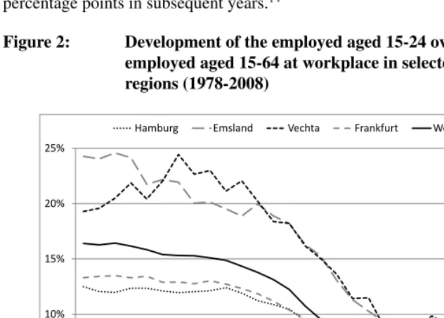
change does not only alter the composition of the population but also the age structure of the labor force we have depicted the share of the young workers (aged 15-24 years) over the total number of workers aged 15-64 years in Figure 2 for the same labor market regions as in Figure 1. The data source is the IAB’s Sample of Integrated Labor Market Biographies (SIAB), see Dorner et al. (2010), a 2% random sample of the individual regis-ter data collected by the Federal Employment Agency (FEA); the reported numbers refer to persons in regular employment subject to social security contributions, at June 30th, the annual record day.12 _{Since the beginning of the 1980s we observe a downward trend,}

i.e., the proportion of the young workforce in Western Germany (continuous dark line) has declined from over 16% to around 6% in the year 2008. This observation corresponds to the strong decrease in cohort sizes at the end of the baby boom generation.13

Figure 1: Population aged 15-24 over population aged 15-64 in selected Western German labor market regions (1978-2009)

0% 5% 10% 15% 20% 25% 30% 35%

1978 1979 1980 1981 1982 1983 1984 1985 1986 1987 1988 1989 1990 1991 1992 1993 1994 1995 1996 1997 1998 1999 2000 2001 2002 2003 2004 2005 2006 2007 2008 2009

Emsland Frankfurt Hamburg Vechta West Germany

12_{In the remainder of the paper, employment always refers to employment that is subject to social security.} 13_{Note that while the relative population of the 15-24 years age group stabilizes after 1994, this is not so much}

(12)

We find differences in labor market developments similar to regional heterogeneity in population developments. The share of young workers has been slightly over 24% in the labor market region Emsland but under 13% in Hamburg in 1978. Over the last decades this share has decreased significantly in Emsland, i.e. by 17 percentage points, whereas the decline is less pronounced in Hamburg (-7 percentage points). The situation in Frankfurt is quite similar to that in Hamburg, whereas in Vechta, the youth has increased until the mid 1980s (to over 24% in 1984) and has experienced a strong decline by 18 percentage points in subsequent years.14

Figure 2: Development of the employed aged 15-24 over the number of employed aged 15-64 at workplace in selected labor market regions (1978-2008)

0% 5% 10% 15% 20% 25%

1978 1979 1980 1981 1982 1983 1984 1985 1986 1987 1988 1989 1990 1991 1992 1993 1994 1995 1996 1997 1998 1999 2000 2001 2002 2003 2004 2005 2006 2007 2008

Hamburg Emsland Vechta Frankfurt West Germany

Source: Institute for Employment Research: SIAB (1975-2008), own calculations.

The proportion of unemployed persons aged 15-24 has decreased in Western Germany until the beginning of the new millennium. Though there are significant differences in the

14_{The developments in population and employment shares differ because the relative employment (employment}

(13)

unemployment levels across the labor market regions, the direction of the developments are quite similar (see Figure 3). After the introduction of the so-called Hartz reforms15

2003 to 2005 the unemployment figures and especially the share of unemployed aged 15-24 have increased strongly in most regions, partly due to changes in the accounting of unemployment.

Figure 3: Development of the unemployed aged 15-24 over the number of unemployed aged 15-64 in selected labor market regions (1978-2008)

0% 5% 10% 15% 20% 25% 30% 35% 40% 45% 50%

1978 1979 1980 1981 1982 1983 1984 1985 1986 1987 1988 1989 1990 1991 1992 1993 1994 1995 1996 1997 1998 1999 2000 2001 2002 2003 2004 2005 2006 2007 2008

Hamburg Emsland Vechta Frankfurt West Germany

Source: Institute for Employment Research: SIAB (1975-2008), own calculations

Overall, the size of the labor market entry cohort (15-24) decreased considerably (about 1.5 million) in the period of concern (1978 to 2008), while at the same time un-employment rose considerably (about 2 millions). By, inadmissibly, considering this

de-15_{The laws for the reform of the German labor market are often denoted as Hartz I-IV. The first three laws}

(14)

scriptive correlation as a causal relationship, we would deduce that smaller cohorts led to increasing unemployment.

Comparing the youth shares across selected labor market regions shows that demo-graphic change and labor market developments proceed differently across the German districts. Overall, the share of employed persons aged 15 to 24 years over the employed persons aged 15 to 64 has decreased until the end of the 1990s and has remained constant in subsequent years. Clearly, the descriptive evidence does not permit us to infer any causal relationship between declining birth cohorts and labor market developments. In order to identify a causal effect, we exploit regional variation and the variation over time in the youth as well as in the workforce, and develop an identification strategy based on exclusion restrictions. However, before conducting the econometric analysis, in the next section, we calculate the compositional direct effect of changes in the age structure as well as in participation on the unemployment rate.

4 Direct effects of demographic changes on the unemployment rate

Transferring the ambiguous results from the cohort crowding literature to cohort shrink-ing implies, on the one hand, that the aggregate unemployment rate is expected to fall due to less competition among entrants on the labor market (Easterlin 1961). On the other hand, theory also suggests that companies may create fewer jobs in regions with a low birth rate so that overall unemployment may increase (Shimer 2001). Since the aggregate unemployment rate is the product of age-specific weights and age-specific unemployment rates, changes in the overall unemployment rate may stem from two sources. First, co-hort sizes may increase or decrease, i.e. the age-specific weights may change (the direct effect), or second, age-specific unemployment rates may vary across years.

In what follows, we calculate the direct effect on unemployment of the composition and participation, across age groups on unemployment, applying the population weights of a base year to the actual age-specific participation and unemployment rates of each year to calculate a counterfactual unemployment rate. The difference to the actual unemploy-ment rate is then called direct effect (Flaim 1990; Shimer 2001). In Section 2, we defined the direct effect of cohort size on unemployment as being simply the difference between the actual unemployment rate and a counterfactual unemployment rate, constructed by ap-plying the population weights of a base year to actual age-specific unemployment rates. The underlying assumption is that age-specific unemployment rates are determined by other factors and thus that the composition shapes the aggregate unemployment rate.

(15)

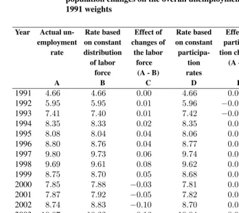
ac-tual age-specific unemployment rates for each year over the available time period (1991-2009) to a labor force for which age components are held constant (here labor force weights from 1991). We then compute the difference between this counterfactual rate (Table 2, column B) and the actual rate (column A) which indicates the amount of change in the overall rate that stems from changes in the composition of the labor force (column C). The results in column C in Table 2 indicate that since the year 2000, the counterfactual unemployment rate based on a constant distribution of the labor force would have been higher than the actual unemployment rate in the same year. Hence, due to changes in the composition of the labor force, the unemployment rate is lower than the situation with no changes in the composition of the labor force. Put differently, the unemployment rate would have been higher if there were no changes in the composition in the age structure of the labor force.16

The effects of changes in labor force participation rates of the various age groups are represented in the next two columns of Table 2. In particular, values in column E are arrived at by subtracting from column A a counterfactual unemployment rate (column D) which is computed by allowing the age-specific unemployment rates and the popula-tion structure to change over time while holding the labor force participapopula-tion rates of the various groups at their 1991 levels.

With respect to changes in participation rates we observe very low values in column E, indicating that the effect of changes of the participation rate is low. Consequently, the overall effect of population changes on the unemployment rate (column F) is very close to the effect of changes of the labor force. The unemployment rate in 2009 would have been 0.22 percentage points higher compared to the actual unemployment rate if there had been no changes in the age structure of the population. Thus, demographic change in Germany (from 1991 to 2009) results in a low but still negative (direct) effect on the overall unemployment rate. To summarize, the direct effect shows that the unemployment rate would have been higher after 2000 if the composition of the population had been the same as in 1991. Thus, this finding can be interpreted as first evidence for a positive relationship between declining cohort sizes and a lower unemployment rate. However, the calculation of such a counterfactual unemployment rate is based on a static approach, i.e. the potential reaction of firms is not considered at all. For this reason, we scrutinize this evidence by some further econometric analysis.

16_{For the calculation of the direct effect, we use a different data source, namely the}_Mikrozensus_{. This is the}

(16)

Table 2: Effect of total compositional changes and of participation and population changes on the overall unemployment rate, based on 1991 weights

Year Actual

un-employment rate Rate based on constant distribution of labor force Effect of changes of the labor force

(A - B)

Rate based on constant participa-tion rates Effect of participa-tion changes

(A - D)

Effect of population changes, the direct effect

(C - E)

A B C D E F

1991 4.66 4.66 0.00 4.66 0.00 0.00

1992 5.95 5.95 0.01 5.96 −0.01 0.01

1993 7.41 7.40 0.01 7.42 −0.01 0.02

1994 8.35 8.33 0.02 8.35 0.01 0.01

1995 8.08 8.04 0.04 8.06 0.02 0.02

1996 8.80 8.76 0.04 8.77 0.03 0.01

1997 9.80 9.73 0.06 9.74 0.06 0.01

1998 9.69 9.61 0.08 9.62 0.07 0.01

1999 8.75 8.70 0.05 8.68 0.07 −0.02

2000 7.85 7.88 −0.03 7.81 0.04 −0.07

2001 7.87 7.92 −0.05 7.82 0.05 −0.10

2002 8.74 8.83 −0.10 8.70 0.03 −0.13

2003 10.07 10.22 −0.16 10.04 0.03 −0.19

2004 11.04 11.26 −0.22 11.03 0.01 −0.23

2005 11.26 11.58 −0.33 11.33 −0.07 −0.26

2006 10.36 10.61 −0.25 10.39 −0.04 −0.21

2007 8.72 8.95 −0.23 8.76 −0.04 −0.19

2008 7.61 7.82 −0.22 7.65 −0.05 −0.17

2009 7.82 8.12 −0.30 7.91 −0.08 −0.22

5 The effect of the youth share on the labor market

5.1 Econometric specifications

(17)

region and the unemployment rate or the employment rate, respectively, in the same re-gion.17 _{Thus, we aim to measure a combined effect of demographic change on}

employ-ment, comprising the indirect effect plus the direct effect from above. We employ relative numbers in the analysis to rule out size effects; in the estimations, each observation is weighted with the fraction of the region’s age population on the total working-age population. The dependent variable, logratei,t, is either the natural log of the

un-employment ratio over all age groups(#unemployed)/(population (age 15-64 years))or the natural log of the employment ratio over all age groups(#employed (at residence))/

(population (age 15-64 years)). We conduct this analysis at a disaggregated regional scale for all Western German labor markets (i = {1, ...,108}) and consider the period from 1993 to 2009t = {1993, . . . ,2009}).18 Demographic change is measured by the (log) size of the labor market entry cohort which we also denote aslog youth share:

log (youth share)_i,t= log

population (age 15-24years) population (age 15-64years)

i,t

The coefficient of interestγ– the elasticity ofratei,tfor the local youth share –

indi-cates the sign and the size of the youth share effect on the unemployment or employment ratio, respectively:

log(rate)i,t=αi+βt+γlog (youth share)_i,t+εi,t (1)

where the coefficientsαin equation (1) capture regional and the coefficientsβ time ef-fects. The random disturbance term is represented byε.

When estimating with OLS, identification of the coefficientγas causal effect requires that the share of the youth population on the overall population does not depend on the un-employment rate. However, the youth share in specification (1) is likely to be endogenous, since individuals relocate across regions due to disparities in labor market conditions. In order to address this endogeneity, we use the cohort size of the same group 15 years ago (lagged birth cohort), when both the persons in the numerator and the denominator were 15 years younger, as our instrument for the local current cohort size. That is, we define

17_{Because of the fast decline in population and employment after reunification, Eastern Germany would be}

particularly interesting to look at. However, both because we do not have access to population data prior to 1991 and as labor markets may have been working differently in the 1990s, we are not able to make any statements about Eastern Germany on the basis of our analysis.

18_{The IV procedure (see below) constrains our sample to the time period from 1993 to 2009. We use the}

(18)

thelagged (log) birth shareas

log (birth share)_i,t₋₁₅= log

_{population (age 0-9 years)}

population (age 0-49 years)

i,t−15

We discuss the validity of the instrument below. Since we consider the population aged 15 to 24 years as the entry cohort, we estimate equation (1) with IV, with the follow-ing equation (2) as first stage regression:

log (youth share)_it=δi+ϕt+µlog (birth share)i,t−15+ψi,t (2)

5.2 Empirical results

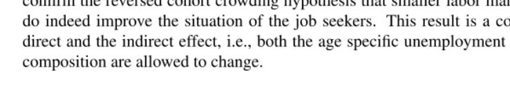
In Table 3 we present the results from our OLS and IV estimations where we regress the log (un)employment ratio on the log youth share (weighted by the population shares of the respective labor market region) as defined above, using heteroscedasticity-consistent standard errors (White 1980). Due to the log-log specification the coefficients can be in-terpreted as elasticities. Our OLS results indicate that a 10 percent decline in the youth share of the population – in 2009 a reduction of roughly 1.7 percentage points – is corre-lated with a 3.96 percent decline in the unemployment ratio. We find a negative elasticity of -0.456 in the employment ratio, i.e. a 10 percent decline in the youth share corresponds with a 4.56 percent increase in the overall employment ratio. Hence, the point estimates confirm the reversed cohort crowding hypothesis that smaller labor market entry cohorts do indeed improve the situation of the job seekers. This result is a combination of the direct and the indirect effect, i.e., both the age specific unemployment rates and the age composition are allowed to change.

Table 3: Results – Basic specifications

Explanatory Variable: Log youth

Log unemployment/population ratio, 1993-2009

Log employment/population ratio (residence, age 15-64), 1999-2009

OLS IV OLS IV

Coefficient 0.3961 1.2758 −0.4561 −0.4569

(0.1698) (0.2383) (0.1045) (0.2167)

Notes: Estimation equations are saturated with region and year dummies. Observations are weighted with popula-tion shares to account for the different size of the regions.

Standard errors are given in parentheses.

(19)

market regions, implying that the actual local cohort size is endogenous. We follow an IV approach to address the potential endogeneity problem, using the relative size of the lagged births cohorts as an instrument for the relative size of the labor market entry co-hort (see equation 2). To be a valid instrument, a variable has to satisfy two conditions: it needs to be sufficiently correlated with the endogenous explanatory variable with suffi-cient variation, and the instrument itself must not be endogenous (or driven by the same omitted factor, facing the same measurement error). The lagged birth rate varies over time and between labor market regions; the annual coefficient of variation varies between 0,09 and 0,042 over the observation period and is slightly above the values for the labor market entry cohorts. In the first stage, the instrument is highly significant with an es-timated coefficient of around 0.5. The partial R-squared mounts to 0.416, the F-statistic for the instrument to 440 in the estimation over the period 1993-2009, while the partial R-squared is 0.338 and the F-statistic for the instrument 271 over the period 1999-2009.

Exogeneity of lagged birth shares with regard to the second stage regression, i.e. its validity as an instrument, is plausible (in an economic interpretation of excluding reverse causality) as long as parents do not relocate due to the anticipated labor market situation fifteen years ahead, which we believe to be not a too restrictive assumption. In addition, the exogeneity assumption might fail if shocks on the (un)employment rate are too persis-tent over timeandif the instrument is affected by the (un)employment rate fifteen years ago. In other words, if a shock on unemployment 15 years ago affected the birth share at that time and is still persisting in today’s unemployment the instrument will not be valid. Local unemployment rates in Germany tend to have a long memory, with the half-life of shocks in an interval between three and thirteen quarters (Patuelli et al. 2012). The enor-mous half-life of more than three years implies that after fifteen years less than five percent of the original amount of the shock is traceable, hardly enough to cause endogeneity in our instrument. We were able to reject that the share of the 0 to 9 to the 0 to 49 population in our sample depends on the (contemporaneous) regional (un)employment rate. Thus, we conclude that these two sources of endogeneity are not likely to be problematic in our case.

The estimated coefficient of the 2SLS model for the youth share effect on the un-employment ratio is much larger when compared to the OLS specification. This is in line with our expectation, since labor mobility tends to equalize labor market differences, thus making the observed partial correlation smaller. The reported elasticity in Table 3 is 1.276, indicating that a 10 percent decrease in the youth share translates into a more than 13 percent decline in the unemployment ratio. The estimated coefficient is statisti-cally significantly positive, but not significantly larger than unity. Employment elasticity remains negative (almost at the same value).

(20)

Thus, our results support the cohort crowding hypothesis, namely that large or small labor market entry cohorts positively or negatively affect unemployment, i.e. an increase or de-crease in the unemployment rate. Consequently, since demographic change in (Western) Germany has been characterized by declining birth cohorts, these results suggest that a re-duction in cohort size had a positive impact on the labor market in the sense that it lowered the unemployment rate and increased the employment rate. In addition, the differences between OLS and IV estimates are consistent with the view that individuals react to the local labor market situation of the region where they grow up by moving to regions with ex-ante lower unemployment. As a consequence, the post-mobility elasticities estimated by OLS are both closer to zero.

5.3 Discussion and robustness checks

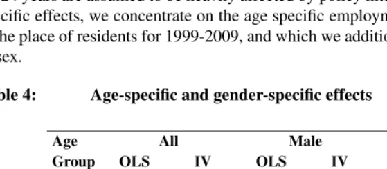
In order to assess whether our results are valid under alternative assumptions we perform several robustness checks. First, we present results for specific age groups, since we would assume that the labor market situation of those aged 15-24 years was affected most by a large entry cohort, while we expect other groups to be affected less. Unfortunately, we do not have access to a full regional time series for age-specific unemployment. In addition, both numerator and denominator of the unemployment rates for the group aged 15-24 years are assumed to be heavily affected by policy interventions. Thus, for the age-specific effects, we concentrate on the age age-specific employment rates, which we observe at the place of residents for 1999-2009, and which we additionally differentiate according to sex.

Table 4: Age-specific and gender-specific effects

Age All Male Female

Group OLS IV OLS IV OLS IV

15-24 -1.3122 -1.2948 -1.2628 -1.5930 -1.2081 -0.9425 (0.1462) (0.2741) (0.1397) (0.3233) (0.1402) (0.2472) 25-49 -0.4342 -0.4557 -0.4362 -0.6600 -0.2960 -0.2107

(0.1003) (0.2101) (0.0834) (0.2308) (0.1123) (0.2109) 50-64 -0.1744 -1.2816 -0.1219 -1.2785 -0.1944 -1.2469

(0.1529) (0.3286) (0.1182) (0.3359) (0.1797) (0.3435) 15-64 -0.4561 -0.4569 -0.4672 -0.6645 -0.3496 -0.1869

(0.1045) (0.2167) (0.0857) (0.2337) (0.1164) (0.2182)

(21)

As expected, the coefficients are largest for the young age group. In addition, gener-ally, male coefficients are larger than female ones and female ones tend to be insignificant. While for OLS the ranking of the age effects is as expected, the IV estimates show rela-tively high values for the oldest age group. It may be the case that older workers benefit from regulations that allow them to retire early more easily when large cohorts enter the labor market, or that firms that observe small cohorts entering try harder to keep their workforce in the face of an upcoming labor shortage. However, we are not able to give an explanation why this doesn’t show up in the OLS estimates, since we do not think that there is strong migration in this age group.

The estimates in specification (1) are likely to have serially and spatially correlated residuals – or to be determined by a serially and spatially lagged dependent variable – because of the persistence and the spatial distribution of the (un)employment rate in Ger-many. Since ignoring serial correlation would provide inefficient estimates of our coeffi-cient of interestγas well as biased standard errors when not using a robust covariance es-timate, we check for serial correlation in the error term of the formi,t =ρi,t−1+ui,t. Put

differently, we account for the possibility that region specific shocks to (un)employment only gradually vanish over time. In order to gain efficiency and to account for autocorre-lation in the error term, we employ a feasible generalized least square (FGLS) estimator with a least-squares estimate forρ, which can be implemented as Prais-Winsten (PW) and/or Cochrane-Orcutt (CO) approach (Greene 2008). Shimer (2001) uses the CO pro-cedure to account only for serial correlation.

However, as our data are observed at a regional level, it is likely that the estimations are also affected by spatial correlation, e.g. because region specific shocks to unemploy-ment (while overall shocks are captured by the time dummies) may affect neighboring regions due to commuting or because of events commonly affecting neighbor regions. In that case, observations cannot be considered independent and estimates may turn out to be, at best, inefficient, or, at worst, biased. Foote (2007) shows that this alters the results for the US labor market considerably. To account for cross-sectional dependencies, we use a row-standardized first-order contiguity matrix (wherein the elementcijcontains the value

1 if regionsiandj have a common border and 0 otherwise; or in the row-standardized version withwij = PNcij

j=1cij) as spatial link matrixW and estimate a model wherein the

residual is assumed to follow a SAR(1) process of the formi,t=λ PN

j=1wij j,t+ui,t.19

The spatial autocorrelation parameter is estimated using the generalized-moments routine

19_{A first-order contiguity spatially autoregressive process}_{= (I}₋_λW₎−1_u_{is equivalent to an infinite order}

spa-tial moving average=P∞

k=0λkWkuwhere the weights used in computing the average decline geometrically

(22)

for random effects panel data provided by Kapoor, Kelejian, and Prucha (2007) which has been shown to be applicable even in a fixed effects specification by Mutl and Pfaffermayr (2011). Like the serial correlation FGLS estimator relying on the parameter estimateρˆ, the parameter estimateλˆcan then be used in a Cochrane-Orcutt transformation to receive a FGLS estimator accounting for spatial correlation.

To establish robustness against joint occurrence of serial and spatial correlation we employ the cluster-based Heteroscedasticity and Autocorrelation consistent Covariance (HAC) estimator provided by Bester, Conley, and Hansen (2011) which is, in panel data, easier to implement than Bartlett-Kernel HAC estimators à la Conley (1999) (which would require different window lengths along the panel dimensions). We formed 14 groups of contingent labor market regions (the smallest group comprises six regions, the largest twelve regions) and split the sample into the periods 1993-1998, 1999-2003 and 2004-2009. That is, standard errors for the unemployment ratio result from grouping in 42 clusters, standard errors for the employment ratio from 28 clusters.20

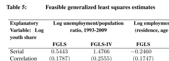
Results for the FGLS estimations, using CO transformation of the data, and HAC in-ference are provided in Table 5. Starting with employment, the spatially corrected FGLS-IV estimate of the effect of the youth on the employment rate shows a virtually unchanged coefficient when compared to the basic IV specification of Table 3, while in the serially adjusted case the coefficient is somewhat smaller. Unfortunately, both estimates of the employment elasticity are not significant at reasonable levels. In the non-instrumented case, the coefficient for spatial correlation is again almost unchanged and significant. In the case of unemployment, starting with serial dependence, the significant coefficients are larger in size when compared to the non-GLS-transformed OLS and IV estimator. When accounting for spatial correlation, the IV regression of the log unemployment ratio on the log youth shows a very similar result as is the case without this correction. The IV results in Table 3 are in the confidence interval of both FGLS-IV estimates. Looking at the HAC inference, we find in general that the standard errors increase compared to Table 3; the general tendency with regard to significance of effects is however stable. Thus, our estimates are not overly sensitive with regard to cross-sectional correlation, in contrast to what has been demonstrated for Shimer’s results by Foote (2007).

Overall, the estimations for the relationship between the youth and unemployment are quite robust across the alternative specifications. Given that the IV specification pro-vided a bigger elasticity in magnitude than the OLS estimation it seems that, as we ex-pected, young workers do in fact respond to labor market differences by moving to low

follow physical structures. However, previous research for Germany found a high degree of similarity between contiguity-based weights and commuting-based weights which reflect economic connectivity between regions.

(23)

unemployment regions and the significant elasticity estimates tend to support the reverse cohort-crowding hypothesis.21

Table 5: Feasible generalized least squares estimates

Explanatory Variable: Log youth share

Log unemployment/population ratio, 1993-2009

Log employment/population ratio (residence, age 15-64), 1999-2009

FGLS FGLS-IV FGLS FGLS-IV

Serial 0.5443 1.4766 −0.2460 −0.1178

Correlation (0.1787) (0.2555) (0.1747) (0.7634)

Spatial 0.1064 1.2993 −0.4617 −0.4824

correlation (0.1178) (0.2268) (0.1631) (0.2685)

HAC (Cluster) 0.3961 1.2758 −0.4561 −0.4569

(0.3976) (0.4923) (0.1735) (0.2953)

So far we used the ratio of unemployed to the working age population as the main unemployment measure, abstracting from the non-participants. This approach has the advantage that the employment and unemployment equations have the same denominator. As a consequence, the differences between the unemployment and employment equation can directly be interpreted as a participation decision in the labor market.22 _{As robustness}

check we use the official unemployment rate which takes into account the labor force participation effects in the denominator. Overall, these results are roughly comparable to those provided above (see Table 6). From this, we can calculate the magnitude of the change in the unemployment rate that is to be expected from the change of the youth share. The youth share declined between 1991 and 2009 by roughly one tenth (from 19.7% of the population in 1991 to 17.6%) and thus we expect a decrease in the unemployment

21_{In a further robustness check, we account simultaneously for cross-sectional dependencies and serial}

corre-lation in the estimation of the covariance matrix using the estimator of Driscoll and Kraay (1998). Compared to the basic OLS specification of Table 3, we arrive at similar, but not identical, point estimates because the ap-proach does not allow weights. The estimate for employment becomes even more significant. Similar results are also obtained for the IV specification in which the first stage is estimated by hand and where the projected value is used in the second stage. It suffers, however, from the fact that standard errors are not estimated consistently in this case.

22_{To see this, imagine that there would be an increase in the working age population of 1 percent without}

(24)

rate of around 2.4% (equivalent to around -0.21 percentage points). Note that this effect is even smaller than the direct effect calculated in Section 3, but the two numbers are not directly comparable since they refer to different unemployment measures.

In addition, as an alternative to the dependent variable "employment ratio" in which we used head counts, we apply the volume measure full-time equivalents, i.e. we mul-tiply the employment spells from SIAB data by their daily exact durations, taking into account their working time status.23 _{The results provided in Table 6 are in line with our}

findings where we used the employment ratio in heads, although the elasticity is some-what smaller. The strong reaction of the employment rate on the youth share is obviously partly compensated for by reactions on working time.

Table 6: Robustness, variable definitions

Variable OLS IV

Official unemployment rate, 1993-2008 0.2381 1.1632

(0.1767) (0.2590)

Full-time equivalent employment rate, −0.2804 −0.4811

1999-2008 (0.0431) (0.0761)

Notes: Estimation equations are saturated with region and year dummies. Observations are weighted with popu-lation shares to account for the different size of the regions. GLS estimates (analogue to Table 5) do not significantly deviate from the OLS and IV results and are available from the authors.

Additionally, whenever possible, we perform estimations over a longer time series to check whether or not the results are stable for alternative lengths of time. We find that the post-adjustment OLS estimation for unemployment for the maximum data horizon (1985-2009) is much closer to the coefficient of the IV estimate. This result does not only hold for the OLS but also for both GLS estimations (with serial and spatial correlation) and points to some instability of the coefficient over time.

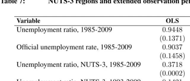
As a further robustness check, we use the 326 West German NUTS-3 regions (exclud-ing West Berlin) instead of the 108 labor market districts as units of observation. The coefficients are given in Table 7 and are, with the exception of the OLS estimate for the unemployment ratio at NUTS-3 level, quite similar to those for the labor market regions. Finally, we use the relative size of the group aged 6 to 14 years to the group aged 6 to 59, lagged nine years as an alternative instrument. The purpose of this is twofold. On the one hand, we are able to additionally consider those years in the late 80s and early 90s with the dramatic decline in the size of the young cohort (see the descriptive part of the paper).

23_{We use 39 hours per week as weight for fulltime employees, 24 hours for individuals employed in part-time}

(25)

Table 7: NUTS-3 regions and extended observation period

Variable OLS IV

Unemployment ratio, 1985-2009 0.9448 N.A.

(0.1371)

Official unemployment rate, 1985-2009 0.9037 N.A.

(0.1458)

Unemployment ratio, NUTS-3, 1985-2009 0.3718 N.A.

(0.0002)

Unemployment ratio, NUTS-3, 1993-2009 0.1421 1.1531

(0.0002) (0.1548)

Employment ratio, NUTS-3, 1999-2009 −0.2283 −0.6379

(0.0002) (0.0848)

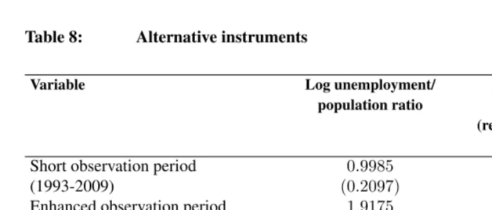
Clearly, this instrument is more difficult to justify at least from an economic perspective, as it requires that people not react to labor market conditions until shortly before they enter the labor market. On the other hand, the second instrument allows us to test the validity of each instrument (assuming validity of the other) and to receive some global statistics on validity of the respective moment conditions. The partial R-squared of the two excluded instruments at the first stage is 0.5384 in the 1993-2009 period and 0.5348 in the 1999-2009 period. The p-value that corresponds to the Hansen J-Statistic amounts to 0.037 in the unemployment-ratio estimation and 0.029 in the employment-ratio esti-mation; that is, joint validity of the two instruments is not rejected at a 99% confidence level. The results are similar to the other instrumental variable results, when we restrict the period of observation to the same time as for the other instrument. For the enhanced observation period the effect on unemployment is considerably larger.

Do the positive relationship between the youth share and the unemployment rate and the (IV) elasticity of around one and the negative elasticity between the youth and the employment ratio of around 0.5 fit together? Since the employment ratio is about ten times the unemployment ratio, we would expect the elasticity of the former to be much smaller than that of the latter. The fact that the numbers are closer than factor 10 implies that the decision to participate in the labor market plays an important role.

(26)

Table 8: Alternative instruments

Variable Log unemployment/

population ratio

Log employment/ population ratio (residence, age 15-64),

only 1999-2009

Short observation period 0.9985 −0.2136

(1993-2009) (0.2097) (0.2041)

Enhanced observation period 1.9175 N.A.

(1987-2009) (0.2142)

Short observation period, two 1.0467 −0.2890

instruments, GMM, (1993-2009) (0.2093) (0.1580)

for the United States. However, it sharply contrasts with Shimer (2001) who comes to the conclusion that a 10 percent increase in the youth share results in 1.5 percent decrease in the unemployment rate. The differences between our results and Shimer’s are not only due to the consideration of cross-sectional dependencies in the econometric specification. Even without this adjustment, the German labor market seems to be affected differently by demographic changes than the US labor market. Future research hopefully can contribute to answering this question.

6 Conclusion

(27)

entry cohorts on employment and on unemployment using regional labor market data for the years 1993 to 2009 (with population data from 1978 to 2009) and the direct effect of the age structure on unemployment for the years 1991-2009. The analysis of the di-rect (compositional) effect demonstrates that the unemployment rate would have been higher if there were no changes in the composition of the age structure. Thus, the coun-terfactual unemployment rate, given the stability of demography, is higher than the actual unemployment rate in Germany. However, the difference (amounting to 0.22 percentage points) is not large. The econometric analysis of the combined effect indicates that there is positive relationship between the youth share and the unemployment ratio (and rate). Given that Germany experiences declining cohort sizes among the young, demographic change is likely to improve the situation of job seekers and thus decrease the overall un-employment rate. This is a robust finding across all our econometric specifications and is also consistent with the evidence of the direct compositional effect.

Results of various statistical tests suggest that our IV estimates provide more credible estimates than OLS. However, it is hard to disentangle the origin of the positive effect of the size of the labor market entry cohort on unemployment as long as we do not dispose of age-specific data. Presumably, it is reasonable to argue that the biggest competition occurs within the age groups (Korenman and Neumark 2000). This is confirmed by the age-specific results for employment. However, the generous early retirement programs in Germany in the 1990s are likely to have influenced the decision of elderly workers whether to stay or to leave the labor market. Again, our age-specific results are in line with this argument. Given our empirical analysis, there is clearly room for further research in at least two directions. First, given that demographic change will alter the population size as well as the age composition in the future, it would be promising to analyze the persistence of the relationship between the youth share and both labor market variables. Second, the institutional framework in each economy may be decisive for the magnitude and the direction of the impact demographic change may have on the labor market.

7 Acknowledgements

(28)

References

Berger, M. (1985). The effect of cohort size on earnings growth: A reexamination of the evidence.Journal of Political Economy93(3): 561–573. doi:10.1086/261315. Bester, C., Conley, T., and Hansen, C. (2011). Inference with dependent data

us-ing cluster covariance estimators. Journal of Econometrics 165(2): 137–151. doi:10.1016/j.jeconom.2011.01.007.

Card, D. and Lemieux, T. (2001). Can falling supply explain the rising return to college for younger men? a cohort-based analysis. The Quarterly Journal of Economics116(2): 705–746.doi:10.1162/00335530151144140.

Conley, T. (1999). GMM estimation with cross sectional dependence. Journal of Econo-metrics92(1): 1–45.doi:10.1016/S0304-4076(98)00084-0.

Dorner, M., Heining, J., Jacobebbinghaus, P., and Seth, S. (2010). Sample of integrated labour market biographies (SIAB) 1975-2008. IAB. (FDZ Datenreport 01/2010).

Driscoll, J. and Kraay, A. (1998). Consistent covariance matrix estimation with spa-tially dependent panel data. Review of Economics and Statistics 80(4): 549–560. doi:10.1162/003465398557825.

Easterlin, R. (1961). The American baby boom in historical perspective. American Eco-nomic Review51: 869–911.

Eckey, H.F., Kosfeld, R., and Türck, M. (2006). Delineation of German labour market regions.Raumforschung und Raumordnung64: 299–309.

Fitzenberger, B. and Kohn, K. (2006). Skill wage premia, employment, and cohort effects: Are workers in Germany all of the same type? IZA. (Discussion paper 2185).

Flaim, P. (1979). The effect of demographic changes on the nation’s unemployment rate. Monthly Labor Review102: 13–23.

Flaim, P. (1990). Population changes, the baby boom and the unemployment rate.Monthly Labor Review113: 3–10.

Foote, C. (2007). Space and time in macroeconomic panel data: Young workers and state-level unemployment revisited. Federal Reserve Bank of Boston. (Working Paper 07-10).

Greene, W. (2008). Econometric Analysis. Upper Saddle River (NJ): Prentice Hall, 5th ed.

(29)

active labour market policy in Germany. Zeitschrift für Arbeitsmarktforschung40(1): 45–64.

Kapoor, M., Kelejian, H., and Prucha, I. (2007). Panel data models with spa-tially correlated error components. Journal of Econometrics 140(1): 97–130. doi:10.1016/j.jeconom.2006.09.004.

Korenman, S. and Neumark, D. (2000). Cohort crowding and youth labor markets: A cross-national analysis. In: Blanchflower, D. (ed.).Youth employment and joblessness in advanced countries, NBER comparative labor markets series. Chicago: University of Chicago Press: 57–105.

Macunovich, D. (1999). The fortunes of one’s birth: Relative cohort size and the youth labor market in the United States. Journal of Population Economics12(2): 215–272. doi:10.1007/s001480050098.

Macunovich, D. (2009). Older men: Pushed into retirement by the baby boomers? IZA. (Discussion Paper 4652).

Mutl, J. and Pfaffermayr, M. (2011). The Hausman test in a cliff and Ord panel model. Econometrics Journal14(1): 48–76.doi:10.1111/j.1368-423X.2010.00325.x.

Ochsen, C. (2009). Regional labor markets and aging in Germany. University of Rostock. (Thünen-Series Working Paper 102).

Patuelli, R., Schanne, N., Griffith, D., and Nijkamp, P. (2012). Persistence of regional unemplyoment: Application of a spatial filtering approach to local labour markets in Germany. Journal of Regional Science52(2): 300–323.

Perry, G. (1970). Changing labor markets and inflation. Brooking Papers on Economic Activity1: 411–441.

Shimer, R. (1999). Why is the U.S. unemployment rate so much lower? NBER Macroe-conomics Annual13: 11–74.

Shimer, R. (2001). The impact of young workers on aggregate labor markets. The Quar-terly Journal of Economics116(3): 969–1007.doi:10.1162/00335530152466287. Siliverstovs, B., Kholodilin, K., and Thiessen, U. (2011). Does aging influence

struc-tural change? Evidence from panel data. Economic Systems 35(2): 244–260. doi:10.1016/j.ecosys.2010.05.004.

Skans, O. (2005). Age effects in Swedish local labor markets. Economics Letters86(3): 419–426.doi:10.1016/j.econlet.2004.09.004.

(30)

di-rect test for heteroskedasticity.Econometrica48(4): 817–838.