Numerical Modeling of River Diversions in the Lower Mississippi River

(1)

University of New Orleans University of New Orleans

ScholarWorks@UNO

University of New Orleans Theses and

Dissertations Dissertations and Theses

5-20-2011

Numerical Modeling of River Diversions in the Lower Mississippi

River

Joao Miguel Faisca Rodrigues Pereira University of New Orleans

Follow this and additional works at: https://scholarworks.uno.edu/td

Recommended Citation Recommended Citation

Pereira, Joao Miguel Faisca Rodrigues, "Numerical Modeling of River Diversions in the Lower Mississippi River" (2011). University of New Orleans Theses and Dissertations. 1309.

https://scholarworks.uno.edu/td/1309

This Dissertation is protected by copyright and/or related rights. It has been brought to you by ScholarWorks@UNO with permission from the rights-holder(s). You are free to use this Dissertation in any way that is permitted by the copyright and related rights legislation that applies to your use. For other uses you need to obtain permission from the rights-holder(s) directly, unless additional rights are indicated by a Creative Commons license in the record and/ or on the work itself.

(2)

Numerical Modeling of River Diversions in the Lower Mississippi River

A Dissertation

Submitted to the Graduate Faculty of the University of New Orleans

in partial fulfillment of the requirements for the degree of

Doctor of Philosophy in

Engineering and Applied Science

by

João Miguel Faísca Rodrigues Pereira

B.S. Technical University of Lisbon, Portugal, 2002 M.S. Technical University of Lisbon, Portugal, 2007

(3)

(4)

ACKNOWLEDGEMENTS

I would like to thank Dr. J. Alex McCorquodale for his guidance, advising and support during this study. Without Dr. McCorquodale‟s kindness, patience and wisdom this document would not have been possible. It was a great privilege to work under his supervision.

I would also like to thank the Lake Pontchartrain Basin Foundation and Dr. John Lopez. The Lake Pontchartrain Basin Foundation funded part of the research herein. Dr. John Lopez gave important technical assistance throughout this study.

I wish to thank the Science and Technology Fund (Louisiana Federal Support) for funding part of this research.

The FVCOM simulations were performed using computational resources (higher performance computing - HPC) provided by the Louisiana Optical Network Initiative (LONI).

Dr. Ehab Meselhe deserves special thanks. Dr. Meselhe is probably the main responsible for me coming to Louisiana. I also thank Dr. Meselhe for the semester I spent at the University of Louisiana at Lafayette working under his supervision and all the technical assistance throughout this Mississippi River study.

I would like to express my gratitude to Dr. Ioannis Georgiou for all the help and support throughout my research. His availability to spend numerous sessions transmitting to me some of his vast knowledge of the numerical models ECOMSED and FVCOM as well as pre-processing and post-processing tools is deeply appreciated.

I would also like to thank the rest of the committee members, Dr. Donald Barbé and Dr. Martin Guillot for their help and suggestions.

I would like to thank Dr. Changsheng Chen and the FVCOM group for allowing me to use their code throughout this study.

I wish to thank Dr. Forrest Holly for several reasons. First of all, for starting the chain of contacts that eventually led me to the University of New Orleans. I also thank Dr. Holly for having the kindness of allowing me to use CHARIMA in my dissertation research. Finally, I thank Dr. Holly for all of the help throughout the modeling process, the technical assistance, the availability to answer all possible questions, and the words of encouragement.

(5)

Dr. Gabriel Retana deserves special thanks for the help with the FVCOM modeling and, most recently, the help given on the ECOMSED post-processing scripts.

Dr. João Rego deserves special thanks for sharing some his work and scripts that helped me during the FVCOM preliminary modeling and testing.

I wish to thank Ms. Mallory Davis for making available her modeling results for use in this study. Her M.Sc. Thesis results are the starting point of part of the research presented herein. I would also like to thank Mallory for her patience and constant availability to answer questions about her work.

I wish to thank my other coworkers at the University of New Orleans during this period: Ms. Rachel Roblin, Mr. Marc Ischen, Ms. Jenni Schindler and Mr. Jeevan Neupane. I also wish to thank Ms. Lynn Brien, Dr. Matthew Bethel, Dr. Sarah Fearnley, Ms. Nathallie Tejeda, Ms. Diane Maygarden and Ms. Heather Gordon-Egger for their precious help with environmental sciences coursework.

I wish to thank all the good friends who helped and encouraged me along the way. In particular, I would like to thank Mr. Boone Larson and Mrs. Brenna Larson, Dr. Gustavo Ferreira, Mr. João Abecasis and Dr. Claes Eskilson for making it easier for me to adapt to a new country and a new reality.

I would like to thank my friends back home for their support along the way and for always finding time to email me. I would like to thank Dr. José Matos Silva in particular for all the encouragement and, for years ago, opening the door for me to enter the hydraulics and numerical modeling world.

(6)

LIST OF FIGURES

Figure 1.1 – Plan View of the Mississippi River Study Area (Source: Visible Earth 2001) ... 2

Figure 4.1 – Flow chart for solution strategy in one time-step for CHARIMA (Source: Holly et al. 1990) ... 36

Figure 4.2 – The sigma coordinate system (Source: HydroQual 2002) ... 39

Figure 4.3 – The locations of the variables on the finite difference grid (Source: HydroQual 2002) ... 40

Figure 4.4 – Schematic of the sediment bed model ... 45

Figure 4.5 – ECOMSED Modeling Framework (Source: HydroQual 2002) ... 49

Figure 4.6 – Simplified Illustration of the interaction between the External and the Internal Mode in ECOMSED (Source: HydroQual 2002) ... 50

Figure 5.1 – ECOMSED Model – Downstream Boundary Mesh ... 57

Figure 5.2 – FVCOM Model – Downstream Boundary Mesh ... 57

Figure 5.3– ECOMSED Model – Stage after 24 h ... 59

Figure 5.4– FVCOM Model – Stage after 24 h ... 60

Figure 5.5 – ECOMSED Model – Depth Averaged Velocity near the D/S Boundary after 24h . 61 Figure 5.6 – FVCOM Model – Depth Averaged Velocity near the D/S Boundary after 24 h ... 61

Figure 5.7– ECOMSED Model – Surface Sand Concentration after 10 h... 62

Figure 5.8– ECOMSED Model – Bottom Sand Concentration after 10 h ... 63

Figure 5.9 – ECOMSED Trapezoidal Channel Cross-Sectional Geometry ... 63

Figure 5.10 – ECOMSED Trapezoidal Channel Model – Depth Averaged Velocity in an intermediate section after 24h ... 64

Figure 5.11 – ECOMSED Trapezoidal Channel Model – Depth Averaged Velocity near the D/S Boundary after 24h ... 65

Figure 5.12– Short Mississippi River Reach Test Domain ... 66

Figure 5.13– Short Mississippi River Reach Test Grids ... 68

Figure 5.14– Longitudinal Profile of the Main Channel Water Discharge - Short Mississippi River Reach Test ... 70

Figure 5.15– Longitudinal Profile of the Main Channel Stage - Short Mississippi River Reach Test ... 70

Figure 5.16– Longitudinal Profile of the Main Channel Sand Concentration - Short Mississippi River Reach Test ... 71

Figure 5.17– Longitudinal Profile of the Main Channel Sand Load - Short Mississippi River Reach Test ... 71

Figure 5.18– Short Mississippi River Reach Test - Surface Velocity at a Bend ... 74

Figure 5.19– Short Mississippi River Reach Test - Bottom Velocity at a Bend ... 76

Figure 5.20– Surface Speed Profile on a Bend - Short Mississippi River Reach Test ... 77

Figure 5.21– Bottom Speed Profile on a Bend - Short Mississippi River Reach Test ... 78

Figure 6.1 – Schematic diagram of the Existing Outflows Topology ... 81

Figure 6.2 – Stage at Belle Chasse for the 1-D Hydrodynamics Calibration – 2008 ... 87

(10)

Figure 6.5 – Stage at Scofield South for the 1-D Hydrodynamics Calibration – 2008 ... 88

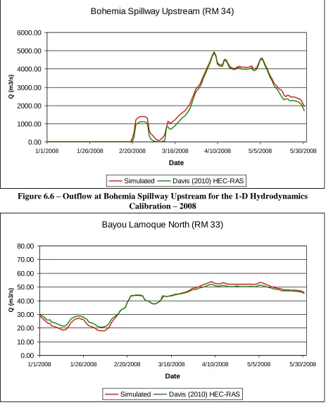
Figure 6.6 – Outflow at Bohemia Spillway Upstream for the 1-D Hydrodynamics Calibration – 2008... 90

Figure 6.7 – Outflow at Bayou Lamoque North for the 1-D Hydrodynamics Calibration – 2008 90 Figure 6.8 – Outflow at Bohemia Spillway Intermediate for the 1-D Hydrodynamics Calibration – 2008... 91

Figure 6.9 – Outflow at Bayou Lamoque South for the 1-D Hydrodynamics Calibration – 2008 91 Figure 6.10 – Outflow at Bohemia Spillway Downstream for the 1-D Hydrodynamics Calibration – 2008... 92

Figure 6.11 – Outflow at Fort St. Philip for the 1-D Hydrodynamics Calibration – 2008 ... 92

Figure 6.12 – Outflow at Baptiste Collette for the 1-D Hydrodynamics Calibration – 2008 ... 93

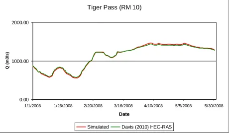
Figure 6.13 – Outflow at Tiger Pass for the 1-D Hydrodynamics Calibration – 2008 ... 93

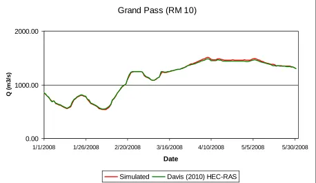
Figure 6.14 – Outflow at Grand Pass for the 1-D Hydrodynamics Calibration – 2008 ... 94

Figure 6.15 – Outflow at West Bay for the 1-D Hydrodynamics Calibration – 2008 ... 94

Figure 6.16 – Outflow at Main Pass for the 1-D Hydrodynamics Calibration – 2008 ... 95

Figure 6.17 – Total Outflow Quadratic Function adjusted to field measurements (Based on Data from Pratt 2009) ... 97

Figure 6.18 – Stage at Belle Chasse for the 1-D Hydrodynamics Validation – 2007 ... 97

Figure 6.19 – Stage at West Pointe-Á-La-Hache for the 1-D Hydrodynamics Validation – 2007 98 Figure 6.20 – Stage at Scofield North for the 1-D Hydrodynamics Validation – 2007 ... 98

Figure 6.21 – Stage at Scofield South for the 1-D Hydrodynamics Validation – 2007 ... 99

Figure 6.22 – Outflow at Bohemia Spillway Upstream for the 1-D Hydrodynamics Validation – 2007... 100

Figure 6.23 – Outflow at Bayou Lamoque North for the 1-D Hydrodynamics Validation – 2007 ... 100

Figure 6.24 – Outflow at Bohemia Intermediate for the 1-D Hydrodynamics Validation – 2007 ... 101

Figure 6.25 – Outflow at Bayou Lamoque South for the 1-D Hydrodynamics Validation – 2007 ... 101

Figure 6.26 – Outflow at Bohemia Downstream for the 1-D Hydrodynamics Validation – 2007 ... 102

Figure 6.27 – Outflow at Fort St. Philip for the 1-D Hydrodynamics Validation – 2007 ... 102

Figure 6.28 – Outflow at Baptiste Collette for the 1-D Hydrodynamics Validation – 2007 ... 103

Figure 6.29 – Outflow at Tiger Pass for the 1-D Hydrodynamics Validation – 2007 ... 103

Figure 6.30 – Outflow at Grand Pass for the 1-D Hydrodynamics Validation – 2007 ... 104

Figure 6.31 – Outflow at West Bay for the 1-D Hydrodynamics Validation – 2007 ... 104

Figure 6.32 – Outflow at Main Pass for the 1-D Hydrodynamics Validation – 2007... 105

Figure 6.33 – Stage at Belle Chasse for the 1-D Mobile-Bed Calibration – 2008 ... 106

Figure 6.34 – Stage at West Pointe-Á-La-Hache for the 1-D Mobile-Bed Calibration – 2008 .. 106

Figure 6.35 – Stage at Scofield North for the 1-D Mobile-Bed Calibration – 2008 ... 107

(11)

Figure 6.37 – Outflow at Bohemia Spillway Upstream for the 1-D Mobile-Bed Calibration –

2008... 108

Figure 6.38 – Outflow at Bayou Lamoque North for the 1-D Mobile-Bed Calibration – 2008 . 108 Figure 6.39 – Outflow at Bohemia Intermediate for the 1-D Mobile-Bed Calibration – 2008 .. 109

Figure 6.40 – Outflow at Bayou Lamoque South for the 1-D Mobile-Bed Calibration – 2008 . 109 Figure 6.41 – Outflow at Bohemia Spillway Downstream for the 1-D Mobile-Bed Calibration – 2008... 110

Figure 6.42 – Outflow at Fort St. Philip for the 1-D Mobile-Bed Calibration – 2008 ... 110

Figure 6.43 – Outflow at Baptiste Collette for the 1-D Mobile-Bed Calibration – 2008 ... 111

Figure 6.44 – Outflow at Tiger Pass for the 1-D Mobile-Bed Calibration – 2008 ... 111

Figure 6.45 – Outflow at Grand Pass for the 1-D Mobile-Bed Calibration – 2008 ... 112

Figure 6.46 – Outflow at West Bay for the 1-D Mobile-Bed Calibration – 2008 ... 112

Figure 6.47 – Outflow at Main Pass for the 1-D Mobile-Bed Calibration – 2008 ... 113

Figure 6.48 – 1-D Existing Outflows – Suspended Sand Concentration at Low Flows – Calibration... 114

Figure 6.49 – 1-D Existing Outflows – Suspended Sand Concentration at Intermediate Flows – Calibration... 115

Figure 6.50 – 1-D Existing Outflows – Suspended Sand Concentration at Peak Flows – Calibration... 115

Figure 6.51 – Suspended Sand Concentration at Belle Chasse for the 1-D Mobile-Bed Calibration – 2008... 116

Figure 6.52 – Suspended Sand Concentration at Myrtle Grove for the 1-D Mobile-Bed Calibration – 2008... 117

Figure 6.53 – Suspended Sand Concentration at Scofield North for the 1-D Mobile-Bed Calibration – 2008... 117

Figure 6.54 – Suspended Sand Concentration at Scofield Intermediate for the 1-D Mobile-Bed Calibration – 2008... 118

Figure 6.55 – Suspended Sand Concentration at Scofield South for the 1-D Mobile-Bed Calibration – 2008... 118

Figure 6.56 – Suspended Sand Load at Belle Chasse for the 1-D Mobile-Bed Calibration – 2008 ... 119

Figure 6.57 – Suspended Sand Load at Myrtle Grove for the 1-D Mobile-Bed Calibration – 2008 ... 120

Figure 6.58 – Suspended Sand Load at Scofield North for the 1-D Mobile-Bed Calibration – 2008... 120

Figure 6.59 – Suspended Sand Load at Scofield Intermediate for the 1-D Mobile-Bed Calibration – 2008... 121

Figure 6.60 – Suspended Sand Load at Scofield South for the 1-D Mobile-Bed Calibration – 2008... 121

(12)

Figure 6.62 – 1-D Simulations - Existing Outflows – Outflows Suspended Sand Concentration at

Intermediate Flows ... 123

Figure 6.63 – Schematic diagram of the Myrtle Grove Case Topology ... 124

Figure 6.64 –Myrtle Grove Outflow – Myrtle Grove Case - 1-D Hydrodynamics Calibration – 2008... 126

Figure 6.65 – Stage at Belle Chasse – Myrtle Grove - 1-D Hydrodynamics Calibration – 2008 127 Figure 6.66 – Stage at West Pointe-Á-La-Hache - Myrtle Grove - 1-D Hydrodynamics Calibration – 2008... 128

Figure 6.67 – Stage at Scofield North – Myrtle Grove – 1-D Hydrodynamics Calibration 2008128 Figure 6.68 – Stage at Scofield South – Myrtle Grove 1-D Hydrodynamics Calibration – 2008129 Figure 6.69 – Stage at Belle Chasse – Myrtle Grove 1-D Mobile-Bed Calibration – 2008... 131

Figure 6.70 – Stage at West Pointe-Á-La-Hache - Myrtle Grove 1-D Mobile-Bed Calibration – 2008... 131

Figure 6.71 – Stage at Scofield North – Myrtle Grove 1-D Mobile-Bed Calibration – 2008 ... 132

Figure 6.72 – Stage at Scofield South – Myrtle Grove 1-D Mobile-Bed Calibration – 2008 ... 132

Figure 6.73 – Suspended Sand Concentration at Myrtle Grove for the 1-D Mobile-Bed Calibration – 2008... 133

Figure 6.74 – Suspended Sand Concentration at Scofield North for the 1-D Mobile-Bed Calibration – 2007/08 ... 134

Figure 6.75 – Suspended Sand Concentration at Scofield Intermediate for the 1-D Mobile-Bed Calibration – 2007/08 ... 134

Figure 6.76 – Suspended Sand Concentration at Scofield South for the 1-D Mobile-Bed Calibration – 2007/08 ... 135

Figure 6.77 – 1-D Simulations – Myrtle Grove – Outflows Suspended Sand Concentration at Peak Flows ... 136

Figure 6.78 – 1-D Simulations – Myrtle Grove – Outflows Suspended Sand Concentration at Intermediate Flows ... 136

Figure 6.79 – Schematic diagram of the Belair Case Topology ... 137

Figure 6.80 – Belair Outflow – Belair Case - 1-D Hydrodynamics Calibration – 2008 ... 139

Figure 6.81 – Stage at Belle Chasse – Belair - 1-D Hydrodynamics Calibration – 2008 ... 140

Figure 6.82 – Stage at West Pointe-Á-La-Hache - Belair - 1-D Hydrodynamics Calibration – 2008... 140

Figure 6.83 – Stage at Scofield North – Belair – 1-D Hydrodynamics Calibration 2008 ... 141

Figure 6.84 – Stage at Scofield South – Belair - 1-D Hydrodynamics Calibration – 2008 ... 141

Figure 6.85 – Stage at Belle Chasse – Belair 1-D Mobile-Bed Calibration – 2008... 144

Figure 6.86 – Stage at West Pointe-Á-La-Hache - Belair 1-D Mobile-Bed Calibration – 2008 144 Figure 6.87 – Stage at Scofield North – Belair 1-D Mobile-Bed Calibration – 2008 ... 145

Figure 6.88 – Stage at Scofield South – Belair 1-D Mobile-Bed Calibration – 2008 ... 145

Figure 6.89 – Suspended Sand Concentration at Myrtle Grove for the Belair 1-D Mobile-Bed Calibration – 2008... 146

(13)

Figure 6.91 – Suspended Sand Concentration at Scofield Intermediate for the Belair 1-D Mobile-Bed Calibration – 2008 ... 147 Figure 6.92 – Suspended Sand Concentration at Scofield South for the Belair 1-D Mobile-Bed Calibration – 2008... 147 Figure 6.93 – 1-D Simulations – Belair – Outflows Suspended Sand Concentration at Peak Flows ... 148 Figure 6.94 – 1-D Simulations – Belair – Outflows Suspended Sand Concentration at

Intermediate Flows ... 149 Figure 7.1 – Sample of Existing ECOMSED Mesh, Bathymetry and Mask at Myrtle Grove (RM 59, RK 94) ... 151 Figure 7.2 – Variation of Bed Shear Stress for the Lower Mississippi River Miles 0 to 300

(Source: El Kheiashy 2007) ... 153 Figure 7.3 – Variation of Bed Form Height for the Lower Mississippi River Miles 0 to 300

(Source: El Kheiashy 2007) ... 153 Figure 7.4 – Stage at Belle Chasse for the ECOMSED Hydrodynamics Calibration at High Flows (2008) ... 154 Figure 7.5 – Stage at West Pointe-Á-La-Hache for the ECOMSED Hydrodynamics Calibration at Low Flows (2008) ... 155 Figure 7.6 – Stage at Scofield North for the ECOMSED Hydrodynamics Calibration at High Flows (2008) ... 155 Figure 7.7 – Stage at Scofield South for the ECOMSED Hydrodynamics Calibration at High Flows (2008) ... 156 Figure 7.8 – Stage at Belle Chasse for the ECOMSED Hydrodynamics Calibration at

Intermediate Flows (2008) ... 156 Figure 7.9 – Stage at West Pointe-Á-La-Hache for the ECOMSED Hydrodynamics Calibration at Intermediate Flows (2008) ... 157 Figure 7.10 – Stage at Scofield North for the ECOMSED Hydrodynamics Calibration at

Intermediate Flows (2008) ... 157 Figure 7.11 – Stage at Scofield South for the ECOMSED Hydrodynamics Calibration at

(14)

Figure 7.20 – Main Channel Total Energy of the Flow at Peak Flows for the Existing Outflows

Case ... 165

Figure 7.21 – Main Channel Kinetic Energy of the Flow at Peak Flows for the Existing Outflows Case ... 165

Figure 7.22 – Main Channel Total Energy Flux of the Flow at Peak Flows for the Existing Outflows Case ... 166

Figure 7.23 – Main Channel Potential Energy Flux of the Flow at Peak Flows for the Existing Outflows Case ... 167

Figure 7.24 – Main Channel Kinetic Energy Flux of the Flow at Peak Flows for the Existing Outflows Case ... 167

Figure 7.25 – Main Channel Water Discharge at Intermediate Flows for the Existing Outflows Case ... 168

Figure 7.26 – Main Channel Total Stage at Intermediate Flows for the Existing Outflows Case ... 169

Figure 7.27 – Main Channel Total Energy of the Flow at Intermediate Flows for the Existing Outflows Case ... 169

Figure 7.28 – Main Channel Kinetic Energy of the Flow at Intermediate Flows for the Existing Outflows Case ... 170

Figure 7.29 – Main Channel Total Energy Flux of the Flow at Intermediate Flows for the Existing Outflows Case... 170

Figure 7.30 – Main Channel Potential Energy Flux of the Flow at Intermediate Flows for the Existing Outflows Case... 171

Figure 7.31 – Main Channel Kinetic Energy Flux of the Flow at Intermediate Flows for the Existing Outflows Case... 171

Figure 7.32 – Suspended Sand Concentration at Peak Flows – Calibration ... 173

Figure 7.33 – Suspended Sand Concentration at Low Flows – Validation ... 173

Figure 7.34 – Suspended Sand Concentration at Intermediate Flows – Validation ... 174

Figure 7.35 – Scofield North (RM 24) Sand Concentration Vertical Profile in the Center of the Channel at Peak Flows ... 174

Figure 7.36 – Modeling versus Field Data (Source: Allison 2010) ... 175

Figure 7.37 – Depth Average Suspended Sand Concentration for ECOMSED Mobile-Bed Calibration at Peak Flows (2008) ... 176

Figure 7.38 – Depth Average Suspended Sand Concentration for ECOMSED Mobile-Bed Calibration at Intermediate Flows (2008) ... 177

Figure 7.39 – Main Channel Suspended Sand Load at Peak Flows for the Existing Outflows Case ... 178

Figure 7.40 – Main Channel Suspended Sand Concentration at Peak Flows for the Existing Outflows Case ... 178

Figure 7.41 – Main Channel Suspended Sand Load at Intermediate Flows for the Existing Outflows Case ... 179

(15)

Figure 7.43 – Existing Outflows – Model Domain - Bed Sediment Thickness Change after 1 day at Peak Flows. Positive values indicate deposition and negative values indicate erosion ... 180 Figure 7.44 – Existing Outflows – Model Domain - Bed Sediment Thickness Change after 10 days at Peak Flows. Positive values indicate deposition and negative values indicate erosion .. 181 Figure 7.45 – Existing Outflows – Belair Area (RM 65) - Bed Sediment Thickness Change after 1 day at Peak Flows. Positive values indicate deposition and negative values indicate erosion 182 Figure 7.46 – Existing Outflows – Myrtle Grove Area (RM 59) - Bed Sediment Thickness

Change after 1 day at Peak Flows. Positive values indicate deposition and negative values

indicate erosion ... 182 Figure 7.47 – Existing Outflows – Belair Area (RM 65) - Bed Sediment Thickness Change after 10 days at Peak Flows. Positive values indicate deposition and negative values indicate erosion ... 183 Figure 7.48 – Existing Outflows – Myrtle Grove Area (RM 59) - Bed Sediment Thickness

Change after 10 days at Peak Flows. Positive values indicate deposition and negative values indicate erosion ... 183 Figure 7.49 – Existing Outflows – Model Domain - Bed Sediment Thickness Change after 1 day at Intermediate Flows. Positive values indicate deposition and negative values indicate erosion ... 184 Figure 7.50 – Existing Outflows – Model Domain - Bed Sediment Thickness Change after 10 days at Intermediate Flows. Positive values indicate deposition and negative values indicate erosion ... 185 Figure 7.51 – Existing Outflows – Belair Area (RM 65) - Bed Sediment Thickness Change after 1 day at Intermediate Flows. Positive values indicate deposition and negative values indicate erosion ... 186 Figure 7.52 – Existing Outflows – Myrtle Grove Area (RM 59) - Bed Sediment Thickness

Change after 1 day at Intermediate Flows. Positive values indicate deposition and negative values indicate erosion ... 186 Figure 7.53 – Existing Outflows – Belair Area (RM 65) - Bed Sediment Thickness Change after 10 days at Intermediate Flows. Positive values indicate deposition and negative values indicate erosion ... 187 Figure 7.54 – Existing Outflows – Myrtle Grove Area (RM 59) - Bed Sediment Thickness

Change after 10 days at Intermediate Flows. Positive values indicate deposition and negative values indicate erosion ... 187 Figure 7.55 – Existing Outflows – Outflows Suspended Sand Concentration at Peak Flows .... 189 Figure 7.56 – Existing Outflows – Outflows Suspended Sand Concentration at Intermediate Flows ... 189 Figure 7.57 – Existing Outflows + Myrtle Grove ECOMSED Mesh and Mask at Myrtle Grove (RM 59, RK 94) ... 190 Figure 7.58 – Existing Outflows + Myrtle Grove (RM 59, RK 94) – Main Channel Kinetic

(16)

Figure 7.60 – Existing Outflows + Myrtle Grove (RM 59, RK 94) – Main Channel Total Energy Flux of the Flow at Peak Flows ... 192 Figure 7.61 – Existing Outflows + Myrtle Grove (RM 59, RK 94) – Main Channel Potential Energy Flux of the Flow at Peak Flows ... 192 Figure 7.62 – Existing Outflows + Myrtle Grove (RM 59, RK 94) – Main Channel Kinetic

Energy Flux of the Flow at Peak Flows ... 193 Figure 7.63 – Existing Outflows + Myrtle Grove (RM 59, RK 94) – Main Channel Suspended Sand Concentration at Peak Flows ... 194 Figure 7.64 – Existing Outflows + Myrtle Grove (RM 59, RK 94) – Main Channel Suspended Sand Load at Peak Flows ... 194 Figure 7.65 – Existing Outflows + Myrtle Grove (RM 59, RK 94) – Main Channel Kinetic

Energy of the Flow at Intermediate Flows ... 195 Figure 7.66 – Existing Outflows + Myrtle Grove (RM 59, RK 94) – Main Channel Total Energy of the Flow at Intermediate Flows ... 196 Figure 7.67 – Existing Outflows + Myrtle Grove (RM 59, RK 94) – Main Channel Total Energy Flux of the Flow at Intermediate Flows ... 196 Figure 7.68 – Existing Outflows + Myrtle Grove (RM 59, RK 94) – Main Channel Potential Energy Flux of the Flow at Intermediate Flows ... 197 Figure 7.69 – Existing Outflows + Myrtle Grove (RM 59, RK 94) – Main Channel Kinetic

Energy Flux of the Flow at Intermediate Flows ... 197 Figure 7.70 – Existing Outflows + Myrtle Grove (RM 59, RK 94) – Main Channel Suspended Sand Concentration at Intermediate Flows ... 198 Figure 7.71 – Existing Outflows + Myrtle Grove (RM 59, RK 94) – Main Channel Sand Load at Intermediate Flows ... 199 Figure 7.72 – Myrtle Grove Area (RM 59) - Bed Sediment Thickness Change after 1 day at Peak Flows. Positive values indicate deposition and negative values indicate erosion ... 200 Figure 7.73 – Myrtle Grove Area (RM 59, RK 94) - Bed Sediment Thickness Change after 10 days at Peak Flows. Positive values indicate deposition and negative values indicate erosion .. 201 Figure 7.74 – Model Domain - Bed Sediment Thickness Change after 1 day at Peak Flows. Positive values indicate deposition and negative values indicate erosion ... 203 Figure 7.75 – Model Domain - Bed Sediment Thickness Change after 10 days at Peak Flows. Positive values indicate deposition and negative values indicate erosion ... 205 Figure 7.76 – Model Domain – Difference between Existing and Myrtle Grove Test Bed

(17)

Figure 7.79 – Model Domain - Bed Sediment Thickness Change after 1 day at Intermediate Flows. Positive values indicate deposition and negative values indicate erosion ... 210 Figure 7.80 – Model Domain - Bed Sediment Thickness Change after 10 days at Intermediate Flows. Positive values indicate deposition and negative values indicate erosion ... 212 Figure 7.81 – Existing Outflows + Myrtle Grove (RM 59, RK 94) – Outflow Suspended Sand Concentrations at Peak Flows ... 213 Figure 7.82 – Existing Outflows + Myrtle Grove (RM 59, RK 94) – Outflow Suspended Sand Concentrations at Intermediate Flows ... 214 Figure 7.83 – Existing Diversions + Belair ECOMSED Mesh and Mask at Belair (RM 65, RK 105) ... 215 Figure 7.84 – Existing Diversions + Belair (RM 65, RK 105)– Main Channel Kinetic Energy of the Flow at Peak Flows ... 216 Figure 7.85 – Existing Diversions + Belair (RM 65, RK 105)– Main Channel Total Energy of the Flow at Peak Flows ... 216 Figure 7.86 – Existing Diversions + Belair (RM 65, RK 105)– Main Channel Total Energy Flux of the Flow at Peak Flows ... 217 Figure 7.87 – Existing Diversions + Belair (RM 65, RK 105)– Main Channel Potential Energy Flux of the Flow at Peak Flows ... 217 Figure 7.88 – Existing Diversions + Belair (RM 65, RK 105)– Main Channel Kinetic Energy Flux of the Flow at Peak Flows ... 218 Figure 7.89 – Existing Diversions + Belair (RM 65, RK 105) – Main Channel Sand

Concentration at Peak Flows ... 219 Figure 7.90 – Existing Diversions + Belair (RM 65, RK 105) – Main Channel Sand Load at Peak Flows ... 219 Figure 7.91 – Existing Diversions + Belair (RM 65, RK 105)– Main Channel Kinetic Energy of the Flow at Intermediate Flows ... 220 Figure 7.92 – Existing Diversions + Belair (RM 65, RK 105)– Main Channel Total Energy of the Flow at Intermediate Flows ... 220 Figure 7.93 – Existing Diversions + Belair (RM 65, RK 105)– Main Channel Total Energy Flux of the Flow at Intermediate Flows ... 221 Figure 7.94 – Existing Diversions + Belair (RM 65, RK 105) – Main Channel Potential Energy Flux of the Flow at Intermediate Flows ... 221 Figure 7.95 – Existing Diversions + Belair (RM 65, RK 105)– Main Channel Kinetic Energy Flux of the Flow at Intermediate Flows ... 222 Figure 7.96 – Existing Diversions + Belair (RM 65, RK 105)– Main Channel Suspended Sand Concentration at Intermediate Flows ... 223 Figure 7.97 – Existing Diversions + Belair (RM 65, RK 105) – Main Channel Suspended Sand Load at Intermediate Flows ... 223 Figure 7.98 – Existing Diversions + Belair (RM 65, RK 105)- Bed Sediment Thickness Change after 1 day at Peak Flows. Positive values indicate deposition and negative values indicate

(18)

Figure 7.99 – Existing Diversions + Belair (RM 65, RK 105) - Bed Sediment Thickness Change after 10 days at Peak Flows. Positive values indicate deposition and negative values indicate erosion ... 226 Figure 7.100 – Model Domain - Bed Sediment Thickness Change after 1 day at Peak Flows. Positive values indicate deposition and negative values indicate erosion ... 228 Figure 7.101 – Model Domain - Bed Sediment Thickness Change after 10 days at Peak Flows. Positive values indicate deposition and negative values indicate erosion ... 230 Figure 7.102 – Model Domain – Difference between Existing and Belair Test Bed Sediment Thickness Change after 10 days at Peak Flows. Positive values indicate that the addition of the Belair Diversion increased deposition. Negative values indicate that the addition of the Belair (RM 65, RK 105) Diversion increased erosion... 231 Figure 7.103 – Belair Area (RM 65, RK 105) - Bed Sediment Thickness Change after 1 day at Intermediate Flows. Positive values indicate deposition and negative values indicate erosion . 232 Figure 7.104 – Belair (RM 65, RK 105)- Bed Sediment Thickness Change after 10 days at

Intermediate Flows. Positive values indicate deposition and negative values indicate erosion . 233 Figure 7.105 – Belair (RM 65, RK 105) - Bed Sediment Thickness Change after 1 day at

Intermediate Flows. Positive values indicate deposition and negative values indicate erosion . 235 Figure 7.106 – Model Domain - Bed Sediment Thickness Change after 10 days at Intermediate Flows. Positive values indicate deposition and negative values indicate erosion ... 237 Figure 7.107 – Existing Outflows + Belair (RM 65, RK 105) Diversion – Outflows Suspended Sand Concentration at Peak Flows ... 239 Figure 7.108 – Existing Outflows + Belair (RM 65, RK 105) – Outflows Suspended Sand

Concentration at Intermediate Flows ... 240 Figure 7.109 – Existing Outflows + Proposed Diversions – Main Channel Water Discharge at

Peak Flows. Proposed Diversions: Jesuit Bend (RM 68, RK 109), Belair (RM 65, RK 105),

Myrtle Grove (RM 59, RK 94), Deer Range (RM 54, RK 87) and Buras (RM 25, RK 40). ... 242 Figure 7.110 – Existing Outflows + Proposed Diversions – Main Channel Total Energy of the

Flow at Peak Flows. Proposed Diversions: Jesuit Bend (RM 68, RK 109), Belair (RM 65, RK

105), Myrtle Grove (RM 59, RK 94), Deer Range (RM 54, RK 87) and Buras (RM 25, RK 40).243 Figure 7.111 – Existing Outflows + Proposed Diversions – Main Channel Kinetic Energy of the

Flow at Peak Flows. Proposed Diversions: Jesuit Bend (RM 68, RK 109), Belair (RM 65, RK

105), Myrtle Grove (RM 59, RK 94), Deer Range (RM 54, RK 87) and Buras (RM 25, RK 40).243 Figure 7.112 – Existing Outflows + Proposed Diversions – Main Channel Total Energy Flux of

the Flow at Peak Flows. Proposed Diversions: Jesuit Bend (RM 68, RK 109), Belair (RM 65, RK

105), Myrtle Grove (RM 59, RK 94), Deer Range (RM 54, RK 87) and Buras (RM 25, RK 40) 244 Figure 7.113 – Existing Outflows + Proposed Diversions – Main Channel Potential Energy Flux

of the Flow at Peak Flows. Proposed Diversions: Jesuit Bend (RM 68, RK 109), Belair (RM 65,

(19)

Figure 7.114 – Existing Outflows + Proposed Diversions – Main Channel Kinetic Energy Flux of

the Flow at Peak Flows. Proposed Diversions: Jesuit Bend (RM 68, RK 109), Belair (RM 65, RK

105), Myrtle Grove (RM 59, RK 94), Deer Range (RM 54, RK 87) and Buras (RM 25, RK 40).245 Figure 7.115 – Existing Outflows + Proposed Diversions – Main Channel Suspended Sand

Concentration at Peak Flows. Proposed Diversions: Jesuit Bend (RM 68, RK 109), Belair (RM

65, RK 105), Myrtle Grove (RM 59, RK 94), Deer Range (RM 54, RK 87) and Buras (RM 25, RK 40). ... 246 Figure 7.116 – Existing Outflows + Proposed Diversions – Main Channel Sand Load at Peak

Flows. Proposed Diversions: Jesuit Bend (RM 68, RK 109), Belair (RM 65, RK 105), Myrtle

Grove (RM 59, RK 94), Deer Range (RM 54, RK 87) and Buras (RM 25, RK 40).... 247 Figure 7.117 – Existing Outflows + Proposed Diversions – Main Channel Water Discharge at

Intermediate Flows. Proposed Diversions: Jesuit Bend (RM 68, RK 109), Belair (RM 65, RK

105), Myrtle Grove (RM 59, RK 94), Deer Range (RM 54, RK 87) and Buras (RM 25, RK 40).248 Figure 7.118 – Existing Outflows + Proposed Diversions – Main Channel Kinetic Energy of the

Flow at Intermediate Flows. Proposed Diversions: Jesuit Bend (RM 68, RK 109), Belair (RM 65,

RK 105), Myrtle Grove (RM 59, RK 94), Deer Range (RM 54, RK 87) and Buras (RM 25, RK 40). ... 248 Figure 7.119 – Existing Outflows + Proposed Diversions – Main Channel Total Energy of the

Flow at Intermediate Flows. Proposed Diversions: Jesuit Bend (RM 68, RK 109), Belair (RM 65,

RK 105), Myrtle Grove (RM 59, RK 94), Deer Range (RM 54, RK 87) and Buras (RM 25, RK 40). ... 249 Figure 7.120 – Existing Outflows + Proposed Diversions – Main Channel Total Energy Flux of

the Flow at Intermediate Flows. Proposed Diversions: Jesuit Bend (RM 68, RK 109), Belair (RM

65, RK 105), Myrtle Grove (RM 59, RK 94), Deer Range (RM 54, RK 87) and Buras (RM 25, RK 40). ... 250 Figure 7.121 – Existing Outflows + Proposed Diversions – Main Channel Potential Energy Flux

of the Flow at Intermediate Flows. Proposed Diversions: Jesuit Bend (RM 68, RK 109), Belair

(RM 65, RK 105), Myrtle Grove (RM 59, RK 94), Deer Range (RM 54, RK 87) and Buras (RM 25, RK 40). ... 250 Figure 7.122 – Existing Outflows + Proposed Diversions – Main Channel Kinetic Energy Flux of

the Flow at Intermediate Flows. Proposed Diversions: Jesuit Bend (RM 68, RK 109), Belair (RM

65, RK 105), Myrtle Grove (RM 59, RK 94), Deer Range (RM 54, RK 87) and Buras (RM 25, RK 40). ... 251 Figure 7.123 – Existing Outflows + Proposed Diversions – Main Channel Suspended Sand

Concentration at Intermediate Flows. Proposed Diversions: Jesuit Bend (RM 68, RK 109), Belair

(RM 65, RK 105), Myrtle Grove (RM 59, RK 94), Deer Range (RM 54, RK 87) and Buras (RM 25, RK 40). ... 252 Figure 7.124 – Existing Outflows + Proposed Diversions – Main Channel Suspended Sand Load

at Intermediate Flows. Proposed Diversions: Jesuit Bend (RM 68, RK 109), Belair (RM 65, RK

(20)

Figure 7.125 – Proposed Diversions – Belair Area (RM 65, RK 105) - Bed Sediment Thickness Change after 1 day at Peak Flows. Positive values indicate deposition and negative values

indicate erosion ... 254

Figure 7.126 – Proposed Diversions – Myrtle Grove Area (RM 59, RK 94) - Bed Sediment Thickness Change after 1 day at Peak Flows. Positive values indicate deposition and negative values indicate erosion ... 255

Figure 7.127 – Proposed Diversions – Belair Area (RM 65, RK 105) - Bed Sediment Thickness Change after 10 days at Peak Flows. Positive values indicate deposition and negative values indicate erosion ... 256

Figure 7.128 – Proposed Diversions – Myrtle Grove Area (RM 59, RK 94) - Bed Sediment Thickness Change after 10 days at Peak Flows. Positive values indicate deposition and negative values indicate erosion ... 257

Figure 7.129 – Model Domain – Difference between Existing and Proposed Test Bed Sediment Thickness Change after 10 days at Peak Flows. Positive values indicate that the addition of the Proposed Diversions increased deposition. Negative values indicate that the addition of the Proposed Diversions increased erosion... 259

Figure 7.130 – Proposed Diversions – Belair Area (RM 65, RK 94) - Bed Sediment Thickness Change after 1 day at Intermediate Flows. Positive values indicate deposition and negative values indicate erosion ... 260

Figure 7.131 – Proposed Diversions – Myrtle Grove Area (RM 59, RK 94) - Bed Sediment Thickness Change after 1 day at Intermediate Flows. Positive values indicate deposition and negative values indicate erosion ... 261

Figure 7.132 – Proposed Diversions – Belair Area (RM 65, RK 105) - Bed Sediment Thickness Change after 10 days at Intermediate Flows. Positive values indicate deposition and negative values indicate erosion ... 262

Figure 7.133 – Proposed Diversions – Myrtle Grove Area (RM 59, RK 94) - Bed Sediment Thickness Change after 10 days at Intermediate Flows. Positive values indicate deposition and negative values indicate erosion ... 263

Figure 7.134 – Existing Outflows + Proposed Diversions – Outflows Suspended Sand Concentration at Peak Flows ... 265

Figure 7.135 – Existing Outflows + Proposed Diversions – Outflows Suspended Sand Concentration at Intermediate Flows ... 265

Figure 8.1 – Rectangular Channel Longitudinal Profile with 1-D Models ... 267

Figure 8.2 – Stage at Scofield North with different time-steps... 268

Figure 8.3 – Outflow at the Main Pass with different time-steps ... 269

Figure 8.4 – Bed-load concentration for different time-steps (Mobile-Bed) ... 270

Figure 8.5 – Suspended Load concentration for different time-steps (Mobile-Bed) ... 270

Figure 8.6 – Cumulative Degradation for different time-steps (Mobile-Bed) ... 271

Figure 8.7 – Volume out of a reach in one-time step for different time-steps (Mobile-Bed) ... 272

Figure 8.8 – Suspended Load Concentration with for different time-steps (Rigid Bed) ... 273

(21)

Figure 8.10 – 2008 Hourly Stage Data - Examples of Inconsistent Measurements ... 278 Figure 8.11 – 1-D Modeling – Main Channel Suspended Sand Concentration at Myrtle Grove (RM 59) for the Tested Scenarios – 2008 Calibration ... 283 Figure 8.12 – 1-D Modeling - Main Channel Suspended Sand Concentration at Scofield

Intermediate (RM 20) for the Tested Scenarios – 2008 Calibration ... 283 Figure 8.13 – 3-D Modeling - Comparison of Total Energy Line for Existing River alone, with an

Intermediate Diversion and with a Large Diversion at High River Flows. Tested Diversions:

Belair (RM 65, RK 105 and Myrtle Grove (RM 59, RK 94) ... 285 Figure 8.14 – 3-D Modeling - Comparison of Kinetic Energy Line for Existing River alone, with

an Intermediate Diversion and with a Large Diversion at High River Flows. Tested Diversions:

Belair (RM 65, RK 105 and Myrtle Grove (RM 59, RK 94) ... 285 Figure 8.15 - 3-D Modeling - Comparison of Suspended Sand Load for Existing River alone,

with an Intermediate Diversion and with a Large Diversion at High River Flows. Tested

Diversions: Belair (RM 65, RK 105 and Myrtle Grove (RM 59, RK 94) ... 286 Figure 8.16 – 3-D Modeling - Outflows Suspended Sand Concentration at Peak Flows for the Tested Scenarios ... 287 Figure 8.17 – 3-D Modeling – Main Channel Suspended Sand Concentration at Peak Flow for

the Tested Scenarios. Proposed Diversions: Jesuit Bend (RM 68, RK 109), Belair (RM 65, RK

(22)

LIST OF TABLES

Table 5-1 – Time-Steps and Split for the Short Mississippi River Test ... 68 Table 5-2 – Boundary Conditions for the Short Mississippi River Test ... 69 Table 5-3 – Short Mississippi River Reach Test - Water discharge and Sand concentration in the Diversion ... 69 Table 6-1 – Flow Boundary Conditions - Existing Outflows Case – 1-D Calibration - /2008 ... 81 Table 6-2 – Stage Boundary Conditions - Existing Outflows Case – 1-D Calibration - 2008 ... 82 Table 6-3 – Sand Load Boundary Condition - Existing Outflows Case – 1-D Calibration - 200882 Table 6-4 – Weirs Parameters - Existing Outflows Case – 1-D Hydrodynamics Calibration - 2008 ... 83 Table 6-5 – Gates Parameters - Existing Outflows Case – 1-D Hydrodynamics Calibration - 2007/2008 ... 83 Table 6-6 – Weirs Parameters - Existing Outflows Case – 1-D Mobile-Bed Calibration -

2007/2008 ... 84 Table 6-7 – Gates Parameters - Existing Outflows Case – 1-D Mobile-Bed Calibration -

(23)

(24)

NOMENCLATURE

Symbol Description Units

C Mean sediment concentration of

suspended sediment

M/L3

T

C Sediment flux concentration (sediment

mass flux per unit mass flow rate)

M/L3/M

*

R0 Parameter for initiation of sediment

transport in Iwagaki Formulation

Dimensionless

* e

R Particle Reynolds Number Dimensionless

i

u Mean flow velocity L/T

W~ Wall proximity function Dimensionless

Divergence operator

∂ Partial differential operator

A Cross-sectional Area L2

a Reference level above the bed L

a Empirical constant for Power

equations

Dimensionless

a0 Constant depending upon bed

properties for resuspension of cohesive sediment

Dimensionless

a0, a1, a2, a3 Empirical coefficients for TLTM

modified formulation

Dimensionless

AH Horizontal mixing coefficient for heat

and salinity

Dimensionless

AM Horizontal mixing coefficient for

momentum

Dimensionless

Ap Peak orbital amplitude L

B Width of the section affected by

bedload transport

L

b Empirical constant for Power

equations

Dimensionless

b1, b2 Coefficient calibrations for Karim‟s

Hiding Factor Equation

Dimensionless

bs

C Suspended load concentration;

Constant used for determination of reference level above the bed

M/L3

Dimensionless

c’ Fluctuating component of sediment

concentration

(25)

C0 Shallow water wave speed;

Maximum volumetric bed sediment concentration

L/T

C1 Cohesive suspended sediment

concentration near the sediment-water interface

M/L3

c1, c2, c3, c4 Coefficients in Ackers-White

Total-Load Predictor

Dimensionless

C2 Near-bed suspended sediment

concentration

M/L3

c5, c6, c7 Empirical coefficients in Karim and

Kennedy flow resistance equation

Dimensionless

CD Drag coefficient Dimensionless

Cf Drag (friction) coefficient Dimensionless

cs Vertical concentration of the

suspended particles

M/L3

Cs(i,j,k) Sediment Concentration in element

(i,j) for level k

M/L3

Csa Sediment concentration at reference

level a

M/L3

Cz Concentration of suspended sediment

in the lowest σ layer

M/L3

d Particle diameter L

D Total water column depth L

d* Dimensionless grain diameter Dimensionless

D* Non-dimensional particle parameter Dimensionless

D1 Depositional Flux M/L2/T

D2 Non-cohesive sediment depositional

flux

D50 Median diameter of sediment L

dgr Dimensionless grain diameter Dimensionless

Dj Sediment diameter for particle size j L

Dk Effective particle diameter L

dQ(i,j,k) Water discharge for level k in element (i,j)

L3/T

dQs(i,j,k) Sediment load for level k in element

(i,j)

M/T

Du Representative diameter of bed

material

L

DZ(k) Fraction of flow depth attributed to level k

(26)

E Resuspension flux; Total energy head

L

Ek Resuspension rate of sediment of class

k

M/L2/T

Etot Total resuspension rate M/L2/T

f Coriolis Parameter T-1

F F-factor Dimensionless

Fgr Sediment mobility number Dimensionless

FH Hydrodynamic force M/L/T2

fk Fraction of class k sediment in the

cohesive bed

Dimensionless

Fs Horizontal diffusion for salinity

Fx Horizontal viscosity

Fy Horizontal diffusion

Fθ Horizontal diffusion for temperature

G Water column shear stress M/L/T2

g Acceleration of gravity L/T2

gs Bed-material discharge in weight per

unit width

M/L

H Total Energy Head L

H Bottom depth relative to z = 0 L

h Mean Flow depth;

Flow depth

L L

hm Mean flow depth L

Hs Wave height L

K Conveyance L3/T

ke Kinetic energy term L

KH Vertical eddy diffusivity for turbulence

mixing of heat and salt

L2/T

KM Vertical eddy diffusivity of turbulent

momentum mixing

L2/T

Ks Manning-Strickler Coefficient L3T

ks Nikuradse roughness height L

L Wave length L

l turbulence macroscale L

L(i,j) Space-step of element (i,j) normal to the direction of the flow

L

m Constant dependent upon the

depositional environment

(27)

n Manning‟s coefficient;

Porosity of bed material;

Constant dependent upon the

depositional environment

L1/3/T

Dimensionless Dimensionless

n’ Manning‟s coefficient component due

to particle roughness

L1/3/T

n’(i,j) Manning‟s coefficient for element (i,j) L1/3

/T

n’’ Manning‟s coefficient component due

to bed forms

L1/3/T

ni Manning‟s coefficient for a certain

sub-section i

L1/3/T

P Pressure;

Power

M/L/T2

ML2/T

P1 Probability of deposition Dimensionless

Pi Wetted Perimeter for a certain

sub-section i

L

Pke Kinetic Energy Power ML2/T

Ptj Proportion of size fraction j in the bed

material

Dimensionless

Q Water discharge L3/T

q Lateral inflow;

Water discharge per unit width

L3/T/L

q2 Turbulent kinetic energy L2/T2

qd Sediment flux due to deposition M/L2

qe Sediment flux due to erosion M/L2

Qs Volumetric bedload sediment

discharge; Sediment load

L3/T M/T

Qss Volumetric suspended load sediment

discharge;

Suspended sediment load

L3/T M/T

qs Total bed-material load;

Sediment discharge per unit width; Suspended load flux

L3/T/L

qsb Bed load;

Volumetric solid discharge per unit width

M/L2

L2/T

qss Suspended load L2/T

qsw Wash load L2/T

qsw Total sediment discharge for particle

size j

(28)

R Hydraulic Radius L

r(I,J) Roughness factor for element (I,J) Dimensionless

Rh Hydraulic Radius L

Rh’ Hydraulic Radius component for the

particle roughness

L

Rh’’ Hydraulic Radius component for the

bed forms

L

S Sediment source or sink within the

solution domain other than the boundaries;

Salinity

M/L3/T

M/M [ppt]

s Specific gravity of the particles Dimensionless

Sf Steady-State Energy or Friction Slope Dimensionless

T Wave period;

Transport Stage parameter

T

Dimensionless

t Time T

Td Time after deposition T

U Mean flow velocity L/T

u Velocity component in the xx

direction;

Near bed velocity

L/T

u* Shear Velocity L/T

u*’ Shear Velocity due to particle

roughness

L/T

u*’’’ Shear Velocity due to bedforms L/T

u*cr bed Critical shear velocity near the bed L/T u*cr sus Critical shear velocity for resuspension L/T

Uc Critical Velocity for beginning of

sediment motion

L/T

ui Instantaneous flow velocity L/T

Up Near bed orbital velocity L/T

V(i,j,k) Component of velocity normal to the face of the element (i,j) through which water is flowing for level k

L/T

Vb Velocity in the grid point nearest the

bottom

L/T

vss Settling velocity of suspended particles L/T

w Vertical velocity component in the zz

direction

L/T

w’ Fluctuating velocity component in the

vertical direction

L/T

(29)

Wp Submerged weight of a particle ML/T2

Ws Settling velocity of the sediment

particles

L/T

Ws,1 Settling velocity of cohesive

suspended sediment flocs

L/T

Ws,2 Settling velocity of non-cohesive

suspended sediment particles

L/T

x Abscissa measured along the river;

Spatial component;

L L

y Water surface elevation

Spatial component

L L

Z Rouse Exponent Dimensionless

z Bed Elevation;

Spatial Vertical Component;

Flow depth at the center of the bottom layer

L L L

Z’ Suspension Parameter Dimensionless

Z0 Bottom Friction L

zb Grid point nearest the bottom L

α Coefficient in Smagorinsky

Parameterization

Dimensionless

β Β-factor Dimensionless

γ Specific weight of water ML/T2/M3

γf Specific weight of a fluid ML/T2/M3

γs Specific weight of sediment ML/T2/M3

Δt Time-step T

Δx Horizontal grid spacing in the xx

direction

L

Δy Horizontal grid spacing in the yy

direction

L

Δσ Vertical Increment which varies with

thickness

L

ε Resuspension Potential M/L2

εj Exposure correction factor Dimensionless

εs Diffusivity of the suspended particles L2/T

η Free surface elevation relative to z = 0 L

θ Potential Temperature (or in situ

temperature) for shallow water

equations; Wave direction

°C

θc Current direction

(30)

κ Prandtl Number Dimensionless

ν Kinematic Viscosity;

Velocity component in the yy direction L2/T L/T

ρ Fluid Density L/M3

ρo Reference Density L/M3

ρs Sediment Density L/M3

τ Bottom Shear stress M/L/T2

τ* Dimensionless shear stress Dimensionless

τ*cr Critical Dimensionless shear stress Dimensionless

τ’ Bottom Shear stress due to particle

roughness

M/L/T2

τ’’ Bottom Shear stress due to bedforms M/L/T2

τ0 Total Bottom Shear Stress;

Average bed level shear stress

M/L/T2

τ0c Critical Total Bottom Shear Stress M/L/T2

τb Bottom Shear Stress M/L/T2

τc Critical shear stress for erosion M/L/T2

τd Critical shear stress for deposition M/L/T2

τzx Dispersivity M/L/T2

ψ Dimensionless intensity of shear stress

applied upon the solid particles

Dimensionless

ω Dummy variable for Partheniades

formulation

Dimensionless

Гs Diffusion coefficient L2/T

Ф Intensity of sediment discharge;

Difference between wave direction and current direction;

Ф-Factor

Dimensionless

(31)

ABSTRACT

The presence of man-made levees along the Lower Mississippi River (MR) has significantly reduced the River sediment input to the wetlands and much of the River‟s sediment is now lost to the Gulf of Mexico. The sediment load in the River has also been decreased by dams and river revetments along the Upper MR. Freshwater and sediment diversions are possible options to help combat land loss. Numerical modeling of hydrodynamics and sediment transport of the MR is a useful tool to evaluate restoration projects and to improve our understanding of the resulting River response. The emphasis of this study is on the fate of sand in the river and the distributaries.

A 3-D unsteady flow mobile-bed model (ECOMSED; HydroQual 2002) of the Lower MR reach between Belle Chasse (RM 76) and downstream of Main Pass (RM 3) was calibrated using

field sediment data from 2008 – 2010 (Nittrouer et al. 2008; Allison, 2010). The model was used to

simulate River currents, diversion sand capture efficiency, erosional and depositional patterns with and without diversions over a short period of time (weeks). The introduction of new diversions at different locations, e.g., Myrtle Grove (RM 59) and Belair (RM 65), with different geometries and

with different outflows was studied. A 1-D unsteady flow mobile-bed model (CHARIMA; Holly et

al. 1990) was used to model the same Lower MR reach. This model was used for longer term

simulations (months).

The simulated diversions varied from 28 m3/s (1,000 cfs) to 5,700 m3/s (200,000 cfs) for

river flows up to 35,000 m3/s (1.2x106 cfs). The model showed that the smaller diversions had little

impact on the downstream sand transport. However, the larger diversions had the following effects: 1) reduction in the slope of the hydraulic grade line downstream of the diversion; 2) reduction in the available energy for transport of sand along distributary channels; 3) reduced sand transport capacity in the main channel downstream of the diversion; 4) increased shoaling downstream of the diversion; and 5) a tendency for erosion and possible head-cutting upstream of the diversion.

(32)

1) INTRODUCTION

1.1 Background

The Mississippi River (MR) has been, since the 1800s, a major natural, economic, and industrial resource for the United States. Historically, the MR was a major source of sediment, freshwater, and nutrients to the Louisiana coast. However, the installation of the levee system, along with the dams, and navigation works, prevents the replenishment of the sediment to the delta. The Louisiana‟s coastal wetlands have been deprived of most of their historic sediment load (about 120 million tons annually), which the river is now transporting to the Gulf of Mexico (Allison and

Meselhe,2010; Parker and Sequeiros 2006).

In order to restore the delta, or at least re-direct part of the sediment being lost, several options are available. One of the most attractive options is the use of river diversions to create new areas of deposition (Parker and Sequeiros 2006). The numerical modeling of hydrodynamics and sediment transport of the MR can be very useful in assessing the potential impacts and behavior of

this type of restoration projects for the Louisiana coast (Meselhe et al. 2005).

This study includes the one-dimensional and three-dimensional modeling of the Lower MR reach from Belle Chasse, LA (RM 76, RK 121) to downstream of the Main Pass, LA (RM 3, RK 5) as shown in Figure 1.1. Due to the presence of flood protection levees, there are no significant inflows along the reach. There are several existing diversions, e.g. White Ditch, Naomi, West Bay and Bayou Lamoque. The east bank of the River downstream of Bohemia (RM 48, RK 77) has a natural levee, which overtops during high flow periods.

In 2008 and 2009, Pereira et al. (2009) used HEC-RAS (USACE 2008), a 1-D quasi-unsteady

flow model, to model the bed material transport of the studied MR reach. Davis (2010) developed a HEC-RAS hydrodynamics unsteady flow application from Tarbert Landing (RM 306, KM 492) to the Gulf of Mexico. A 3-D model is now needed to estimate dredging river currents, depositional patterns, tides and salinity intrusion.

(33)

Figure 1.1 – Plan View of the Mississippi River Study Area (Source: Visible Earth 2001)

1.2 Statement of the Problem

The interaction between sediment and flow has been extensively studied since the 1940s. Vito Vanoni, Hans Albert Einstein, John Kennedy, Hunter Rouse, and Daryl Simons are among the prominent researchers in this field (Barkdoll and Duan 2008).

(34)

turbulence on sediment movement, require further experimental, field, and numerical studies (Barkdoll and Duan 2008).

Since the 1980s, a large number of computational hydrodynamic/sediment transport models have been developed. With the rapid developments in numerical methods for fluid mechanics, 3-D sediment computational modeling has become a much more attractive tool for studying the sediment

transport in such different environments as rivers, lakes, and coastal areas (Papanicolaou et al. 2008).

Unlike physical models, computational models are adaptable to different physical domains and are not subject to distortion effects.

The Lower Mississippi River is a very particular environment. During lower flows, it is mostly dominated by the presence of cohesive sediment, requiring the use of cohesive sediment formulations when performing the numerical modeling of the system. Under high flow conditions, when most of the coarser sediments are transported, the river bed behaves essentially like a non-cohesive sediment bed, requiring very different formulations for the calculation of erosion and deposition rates. This unique setting makes the Lower MR both an interesting and extremely difficult environment for the multidimensional numerical modeling of the sediment transport.

In the last few decades, several modeling efforts have been devoted to the Lower Mississippi River. The United States Army Corps of Engineers (USACE) used TABS-MD (Donnel and Letter 1991) to model a portion of the Lower MR that includes the Head of Passes and 10 miles of the main channel and used CH3D-SED to evaluate dredging and channel evolution issues in the Lower MR. Spasojevic and Holly (1994) incorporated a 2-D mobile bed technique into the CH3D model to simulate the sediment transport at the Old River Structure. Barbé, Fagot and McCorquodale (2000) applied HEC-6 to the Lower MR to determine the sensitivity of dredging requirements to flow and

relative sediment diversions (Meselhe et al. 2005). Meselhe et al. (2006) used the 1-D model Mike11

(DHI 2004) to model the Lower MR bed-material transport from Tarbert Landing, MS (RM 306) to

Venice, LA (RM 11). Pereira et al. (2009) used HEC-RAS (USACE 2008) to model the bed material

transport of the studied MR reach. Davis (2010) used HEC-RAS (USACE 2008) for the 1-D unsteady flow modeling of the hydrodynamics of the Lower MR from Tarbert Landing to the Gulf of Mexico.

A review of various publications concerned with the river hydrologic characteristics and several river-modeling applications, e.g. Demuren (1993) and Corti and Pennati (2000), indicated that complex flow patterns of three-dimensional nature characterize the hydrodynamics of the Lower MR. Therefore, a 3-D model is required to provide information on the river‟s secondary motion, the

sediment distribution in the water column and the modeling of the salt water wedge (Meselhe et al.

2005).

(35)

ECOMSED will serve as a tool to study the non-cohesive sediment transport, which will be done by using the van Rijn (1984) entrainment function.

1.3 Objectives

The main objective of this study is to develop a three-dimensional hydrodynamic and non-cohesive sediment transport model for the Lower MR.

The specific objectives of the study are:

 To determine the distribution of non-cohesive sediment for the Lower MR under the existing

conditions and with the introduction of new river diversions proposed by the MLODS Study (Lopez and LPBF 2008). Four different scenarios will be tested:

1. Existing Conditions

2. Existing Conditions plus a medium size diversion (850 m3/s; 30,000 cfs) at Myrtle

Grove (RM59)

3. Existing Conditions plus a large size diversion (5,700 m3/s; 200,000 cfs) at Belair

(RM65)

4. Existing Conditions plus the multiple diversions proposed in the MLODS Study

(Lopez and LPBF 2008) with modification to the existing passes.

 To develop a three-dimensional model for simulating the non-cohesive sediment transport in

the Lower MR.

 To develop a one-dimensional model for simulating the non-cohesive sediment transport in

the Lower MR.

 To investigate with the aid of numerical models in the large scale diversion of water and

sediment in a low energy environment.

 To quantify the impact of river diversions in the flow, energy and sediment available in the

system.

1.4 General Methodology and Research Plan

The proposed methodology will be followed to meet the objectives:

1. A literature review will be conducted.

2. A selection criterion will be applied to choose the appropriate one-dimensional and

the three-dimensional numerical models. A description of both the one-dimensional and three-dimensional models, and its capabilities will be provided

3. A three-dimensional, finite-volume, sigma-layer, numerical model capable of

simulating hydrodynamics and dynamics of sediment transport will be selected and set up for some simplified tests (rectangular channel; trapezoidal channel; grid dependency study).

4. The code of the three-dimensional model will be extended to include the calculation

(36)

formulation will be adapted to allow its application to the Lower MR.

5. Calibration and verification of longer term one-dimensional simulations for the MR

will be performed to obtain boundary conditions for the three-dimensional model.

6. The three-dimensional model will be calibrated with base on the available data from

the United States Army Corps of Engineers (USACE) and the United States

Geological Survey (USGS) stations and field data collected by Nittrouer et al. (2008)

and by Allison (2010).

7. The three-dimensional model will be applied to the Lower MR (Belle Chasse, LA

(37)

2) LITERATURE REVIEW

2.1 General

Computational fluid dynamics (CFD) is the analysis of systems involving fluid flow, heat transfer and associated phenomena by means of computer-based simulation. The recent advance on high-performance computing hardware and the introduction of user-friendly interfaces have contributed for a broader use of CFD (Versteeg and Malalasekera 2006).

CFD codes are structured around the numerical algorithms that can tackle fluid flow problems. The codes include a pre-processor, a solver and a post-processor (Versteeg and Malalasekera 2006).

The pre-processing stage involves: a) definition of the geometry of the region of interest, the computational domain; b) the sub-division of the domain into a number of smaller, non-overlapping sub-domains, called grid or mesh of cells; c) the selection of the phenomena that need to be modeled; d) the definition of fluid properties and; e) the specification of appropriate boundary conditions (Versteeg and Malalasekera 2006).

There are three numerical solution techniques: finite difference, finite elements and spectral methods. The finite volume method is a special finite difference formulation. The control volume integration distinguishes the finite volume method from the other CFD techniques. The resulting statements express the (exact) conservation of relevant properties for each finite size cell, making its concepts easier to understand by engineers than the finite elements and spectral methods (Versteeg and Malalasekera 2006). Finite volume formulations can be obtained either by a finite difference basis or a finite element basis. The results are identical for one-dimensional problems (Chung 2002).

The finite difference method has the advantage of allowing a simple code structure and computational efficiency. However, it is limited because of the difficulty in accurately fitting

irregular geometry. (Chen et al. 2007).

Geometry flexibility is the main advantage of the finite elements method. The use of unstructured grids allows the possibility of easily discretizing computational domains corresponding

to very complex flow geometries (Kobayashi et al. 1998). However, the traditional finite elements

method is computationally very expensive and does not provide an explicit way to check the mass

conservation in individual cells during the computation (Chen et al. 2007).