A Comparison Between Fourier Transform Adomian Decomposition Method and Homotopy Perturbation ethod for Linear and Non-Linear Newell-Whitehead-Segel Equations

(1)

AUT J. Model. Simul., 49(2)(2017)227-238 DOI: 10.22060/miscj.2017.12051.4998

A Comparison Between Fourier Transform Adomian Decomposition Method and

Homotopy Perturbation Method for Linear and Non-Linear

Newell-Whitehead-Segel Equations

S. S. Nourazar, H. Parsa, A. Sanjari

Department of Mechanical Engineering, Amirkabir University of Technology, Tehran, Iran

ABSTRACT: In this paper, a comparison among the hybrid of Fourier Transform and Adomian Decomposition Method (FTADM) and Homotopy Perturbation Method (HPM) is investigated. The linear and non-linear Newell-Whitehead-Segel (NWS) equations are solved and the results are compared with the exact solution. The comparison reveals that for the same number of components of recursive sequences, the error of FTADM is much smaller than that of HPM. For the non-linear NWS equation, the accuracy of FTADM is more pronounced than HPM. Moreover, it is shown that as time increases, the results of FTADM, for the linear NWS equation, converges to zero. And for the non-linear NWS equation, the results of FTADM converges to 1 with only six recursive components. This is in agreement with the basic physical concept of NWS diffusion equation which is in turn in agreement with the exact solution.

Review History: Received: 17 October 2016 Revised: 11 March 2017 Accepted: 9 May 2017 Available Online: 21 June 2017 Keywords:

Fourier Transform and Adomian Decomposition Method

Homotopy Perturbation Method Newell–Whitehead-Segel Equation Nonlinear Partial Differential Equation

1- Introduction

Recently, a great deal of attention has been dedicated to the semi-analytical solution to the mathematical differential equations associated with the real-life model that are intrinsically nonlinear. Most of the non-linear differential equations do not possess an analytical solution. The homotopy perturbation method (HPM) was first developed by He [1-4] in 1999. Later HPM as a semi-analytical method was used to solve the nonlinear and non-homogeneous partial differential equations. In 2011, the Newell-Whitehead-Segel (NWS) equation was solved using the Adomian decomposition and multi-quadric quasi-interpolation methods [5, 6]. They deduced that the Adomian decomposition and multi-quadric quasi-interpolation methods are rational methods to solve the NWS equation with a passable precision. Examples of applying homotopy analysis method in fluid mechanics are shown in [7-9]. More recently Nourazar [10,11] in 2012 and 2013, has developed a novel modification to Adomian decomposition method (ADM) and HPM and called them Fourier transform Adomian decomposition method (FTADM) and Fourier transform homotopy perturbation method (FTHPM), respectively. They showed that FTADM and FTHPM are more effective than ADM and HPM, respectively, in solving the non-linear differential equations.

In this work, we solve three different non-homogeneous linear and non-linear partial differential equations, the Helmholtz and NWS equations, using FTADM and HPM and discuss the comparison between the results of FTADM and HPM with the exact solution. The closed form solutions for the three partial differential equations which are the same as the exact solutions are obtained. Furthermore, the trend that the results of FTADM converges to a constant value as time goes to

infinity is compared to that of the HPM. The effectiveness and the validity of FTADM are shown in comparison with HPM. One of the most popular amplitude equations in two-dimensional system is the NWS equation. This model portrays the appearance of the stripe schema in two dimensional systems. The NWS equation models the action and the reaction of the effect of the diffusion term with the non-linear effect of the response term [12].

Now, we assume the popular NWS equation of the following type:

subjected to the one initial condition and two boundary conditions,

where a and b take real values. k and q are positive integers. 2- Basic Idea Of Ftadm

The general formula of one-dimensional non-linear partial differential equations is assumed for illustrating the fundamental concept of the FTADM. Consider the following differential equation [10, 11]:

Usually, the operator E may be decomposed into two parts, the non-linear operator, and the linear operator L ,

The corresponding author; Email: icp@aut.ac.ir

(1)

(2)

(3)

(4)

( ,0)

( ),

(0, )

( ), (0, )

( ),

=

_x

=

u x

f x

u t

g t u

t

h t

(

( , )

)

=

0,

≥

0 and

≥

0. E u x t

x

t

(

( , )

)

+

(

( , )

)

=

( ).

N u x t

L u x t

g x

2 2

( , )

( , ),

where u

and

=

+

−

∂

=

∂

q

t xx

u x t

ku

x t

au x t

bu x t

u

_u

u

(2)

Taking the Fourier transform from both sides of Equation (4), we have

where the symbol F denotes the Fourier transform. With using the concept of ADM [13], the unknown function u(x,t) of the linear operator L in Equation (4) can be decomposed by a series solution as [14],

For the non-linear operator N (Equation (4)), we use the Taylor series expansion to expand the non-linear operator N(u(x,t)) around u0=u(x0,t0) as:

where the superscript n indicates the order of derivative with respect to the interdependent parameter u. Inserting into Equation (7) and reordering terms, we have:

The Equation (8) can be written as the series expansion of the Adomian polynomial An as follows:

where the Adomian polynomials An are defined as,

Inserting Equations (9) and (6) into Equation (5), we obtain:

Where the first five Adomian polynomials are,

Equation (11) may be rewritten by the following equation:

Using Equation (13), we represent the recursive relation as,

The recursive relation (14) can be rewritten as,

Using the Maple package software, the first portion of Equation (15) gives the value of F[u0]. Next applying the

inverse Fourier transform to F[u0] gives the value of u0 that

will define the Adomian polynomial A0 using the first portion

of Equation (12). In the second portion of Equation (15) using the Adomian polynomial A0 will enable us to evaluate the value

of F[u1]. Afterwards applying the inverse Fourier transform

to F[u1] gives the value of u1 that will define the Adomian

polynomial A1 using the second portion of Equation (12) and

so on. This in turn will lead to the complete evaluation of the components of uk, k ≥ 0, upon using different corresponding

parts of Eq. (15) and Eq. (12). 3- Case Study

Now, we clearly solve three partial differential equations, to ascertain the credibility and the effectiveness of the presented method FTADM in the whole limited area of the problem domain. In the first example, the two dimensional Helmholtz equation is solved. This equation emerges directly or indirectly in many wave-related problems arisen from various sciences, engineering, and industrial applications

(

( , )

)

+

(

( , )

)

=

[

( ) ,

]

   

   

F N u x t F L u x t F g x ₍₅₎

(6) (7) (8) (9) (10) (12) (13) (14) (15) (11)

(

)

0 0

,

( , )

.

∞ = ∞ =

=





= 

_



_

∑

n n n n

u

L u x t

L

u

(

)

(

)

( ) 0 0 0

1 ( , )

( ),

!

∞ =

=

∑

−

n n n

N u x t

u u N

u

n

0

∞ =

=

∑

_n _n

u u

0 1 0 2

2 0 1 0

3

3 0 1 2 0 1 0

2

4 0 2 1 3 0

2 4 (4)

1 2 0 1 0

( ( , ))

( ) (

( ))

1 ( )

( )

2!

1 ( )

( )

3!

1 ( ) (

) ( )

2!

_...

1 _{( )}

2!

4!

=

′

+



_′

₊

_′′



₊











_′

₊

_′′

₊

_′′′



₊











_′

₊

_′′

₊







+







_′′′

₊











N u x t

N u

u N u

u u N u

u N u

u

u u N u

u N

u

0

( ( , )) ∞ ,

=

∑

_n n

N u x t A

0 ₀

1 _.

!

= ₌









=

_

_

_

_







∑



n n i

i

d

A

N

u

n d

λ

_λ

(

)

0 0 ( ) . ∞ ∞ = =   ₊  ₌  _ _ _ _ 

∑

i i 

∑

i i

F L u F A F g x

0 0

1 1 0

2

2 2 0 1 0

3

3 3 0 1 2 0 1 0

2

4 4 0 2 1 3 0

2 4 (4)

1 2 0 1 0

( ),

1 ( )

( ),

2!

1 ( )

( )

( ),

3!

1 ( )

( )

2!

1

1 ( )

( ).

2!

4!

=

′

=

′

′′

=

+

′

′′

′′′

=

+





′

′′

=

+

_

+

_

+





′′′

+

A

N u

A u N u

A

u N u

A u N u

u u N u

u N u

A

u N u

u

u u N u

u N

u

0

[ ( )]

0

[ ]

[ ].

∞ ∞

= =

+

=

∑

i

∑

i

i i

F L u

F A

F g

0

1 0

[ ( )] [ ],

[ ( )] [ ] 0.

∞ ∞

= =

=

+ =

∑

i

∑

i

i i

F L u F g F L u F A

0 1 0 2 1 3 2 1

[ ( )]

[ ],

[ ( )]

[ ] 0,

[ ( )]

[ ] 0,

[ ( )]

[ ] 0,

[ ( )]

[

−

] 0.

=

−

=

−

=

−

=

−

=

k k

(3)

[15-17]. In the next examples, the linear and nonlinear NWS equations are solved respectively. The NWS equation models the action and the reaction of the effect of the diffusion term with the non-linear effect of the response term

Example 1.

In Cartesian coordinate systems the two dimensional Helmholtz equation is written as:

where the wave number K is defined as the ratio of the frequency to the wave velocity, and u is the unknown dependent variable indicating the pressure of wave. Here we assume a case where A=1, B=1, C=-1 and K=1 as follows,

A) FTADM

To solve Equation (17) with FTADM, we take the Fourier transform of Equation (17) as,

is Fourier transform of u

w is arbitrary Fourier transform parameter

Inserting the recursive relation (Equation (14)) into Equation (18) we get,

The recursive relation inferred from Equation (19) may be written as:

After solving the recursive relation (20) and taking the

inverse Fourier transform using the Maple package software, we obtain the followings:

Consequently, the series form solution of Equation (17) is,

The Taylor series expansion of ex_{is written as,}

By inserting Equation (23) into Equation (22), Equation (22) can finally be simplified to,

The equation (24) is the real exact solution of Equation (17).

B) HPM

To solve Equation (17) with HPM, we create the following homotopy,

P is homotopy parameter v is homotopy function Or, equivalently,

where u0 is defined as an initial approximation to the solution

of Equation (17).

In this manner, we utilize the homotopy parameter P to expand v as a power series:

The approximate solution of Equation (17) can be obtained by setting P equal to 1, i.e.,

Inserting Equation (28) into Equation (26) and comparing the terms with the same powers of p , we have

(16) (17) (21) (22) (23) (18) (19) (24) (25) (26) (27) (28) (29) (20) 2

( , )  ( , ) _{( , ) 0,}

∂  ∂ _{ +} ∂ ∂ ₊ ₌

 

∂  ∂  ∂  ∂ 

u x y u x y

A B CK u x y

x x y y

( , )

( , ) - ( , ) 0

(0, )

, (0, )

cosh( ),

( ,0)

, ( ,0) 1.

+

=

= +

=

xx yy x y

u x y

u x y u x y

u

y

y u

y

u x

x u x

2

ˆ

( , ) - (1

) ( , )

ˆ

(1

)

cosh( ) 0

ˆ

( ,0) -1/ , ( ,0) - / .

ˆ

+

+ +

+

=

yy

y

u

y

u

y

i y

y

u

i

w

2

2 2

0 0

2

ˆ

( , ) - (1

)

ˆ

( , )

(1

)

cosh( ) 0

ˆ

( ,0) -1/ , ( ,0) - / .

ˆ

∞ ∞

= =

+

+ +

+

=

∑

n

∑

n

n n

y

d

_u

_y

_u

_y

dy

i y i

y

u

i

w

0 2 0 0 2 1 0 1 1 2 2 1 2 2 2 3 2 3

ˆ ( , ) (1

)

cosh( ) 0

ˆ

( ,0) -1/ ,

ˆ

( ,0) - /

ˆ

( , ) - (1

) ( , ) 0

ˆ

( ,0) 0, ( ,0) 0

ˆ

( , ) - (1

) ( , ) 0

ˆ

( ,0) 0,

ˆ

( ,0) 0

ˆ

( , ) - (1

) ( , ) 0

ˆ

ˆ ( ,0) 0

+ +

+

=

+

=

+

=

+

=

yy y yy y yy y yy

u

y

i y i

y

u

i

u

y

u

y

u

y

u

y

u

y

u

y

u

w

,

ˆ

₃

( ,0) 0,

... .

=

y

u

w

0 2 3 1 4 5 2 6 7 3

( , )

(1

)

cosh( )

1

1 ( , )

2!

3!

1

1 ( , )

4!

5!

1

1 ( , )

,

6!

7!

... .

=

+

=

+

=

+

=

+

u x y

y

x

y

u x y

x y

u x y

x y

u x y

x y

2 3

0

( , ) (1 ...) cosh( ). 2! 3!

∞

=

∑

_n = + + + + +

n

x x

u x y u y x x y

0

.

!

∞

=

∑

n x

n

x

e

n

( , )

=

x

+

cosh( ).

u x y

ye

x

y

2 2 2 2

0

2 2 2 2

(1

−

)(

∂

−

∂

)

+

(

∂

+

∂

−

) 0.

=

∂

v

u

v

p

v

y

x

2 2 2 2

0 0

2 2

(

2 2

),

∂

−

=

−

∂

v

u

_{p v}

v

u

y

x

y

0

( , )

0

( , )

( ,0)

=

1 .

=

+

+ × = +

y

v x y

u x y

u x

yu x

x y

2

0 1 2

...

=

+

v v

pv

p v

0 1 2

1

lim

_→

...

=

+ + +

p

u

v v v v

ˆ

u 1

= −

(4)

The above relations give the solution as,

Finally, the solution of Equation (17) is given in a series form by

Example 2.

Consider the NWS equation of the following form:

where a,b∈R ,k and q and are positive integers. Here, let k=1, a=-2 and b=0 for a linear form of NWS as follows:

A) FTADM

The Fourier transform of Equation (34) is expressed as:

Inserting the recursive relation (14) into Equation (35) yields

The recursive relation inferred from Equation (36) can be rewritten as,

After solving the recursive relation (37) and taking the inverse Fourier transform using the Maple package software, we obtain the following:

Consequently, the series form solution of Equation (34) is,

The Taylor series expansion form for e-t_{is written as,}

By inserting Equation (40) into Equation (39), Equation (39) can finally be simplified to

Equation (41) is the real exact solution of Equation (34).

B) HPM

To solve Equation (34) with HPM, we create the following homotopy,

Or, equivalently,

2 2

0 0 0

2 2

2 2 2

1 1 0 0

0

2 2 2

2 2

2 2 1

1

2 2

3 3 2

2 2 2

:

0 :

:

,

....

∂

₋

∂

₌

∂

₊

∂

₌

₋

∂

_{= −}

∂

=

−

∂

v

u

p

y

v

u

v

p

v

y

x

v

p

v

y

x

v

p

v

y

x

(30) (35) (36) (37) (38) (39) (40) (41) (42) (43) (31) (32) (33) (34) 0 2 3 1 4 5 2 6 7 3 8 9 4

( , )

1

1 ( , )

2!

3!

1

1 ( , )

4!

5!

1

1 ( , )

6!

7!

1

1 ( , )

,

8!

9!

...

= +

=

+

=

+

=

+

=

+

v x y

x y

v x y

xy

y

v x y

xy

y

v x y

xy

y

v x y

xy

y

2 3 4

1 ₀

5 6 7

1 1 1

lim

2! 3! 4!

1 1 1

+ ...

5! 6! 7!

∞ → ₌ = = = + + + + + +

∑

i p _i

u v v x y xy y xy

y xy y

( , )

=

( , )

+

( , )

−

q

( , ),

t xx

u x y

ku x t

au x t bu x t

2 ,

0 and

0,

( ,0)

, (0, )

−

, (0, )

−

.

=

−

≥

=

t xx

x t t

x

u u

u x

t

u x

e

u t

e

u

t

e

2

ˆ

( , ) (

2) ( , )

ˆ

(

1) 0,

ˆ( ,0)

[ ].

−

+

−

+

+ =

=

t t x

u

t

u

t

e i

u

F e

w

2

0 0

ˆ ( , ) ( 2) ˆ ( , ) ( 1) 0,

ˆ( ,0) [ ].

∞ ∞

−

= =

+ − + + =

=

∑

t

n n

x

d _u _t _u _t _{e i}

dt

u F e

w w w w

w

0 0

2

1 0 1

2

2 1 2

2

3 2 3

ˆ

( , )

(

1) 0, ( ,0)

ˆ

,

ˆ

( , ) (

2) ( , ) 0,

ˆ

( ,0) 0,

ˆ

( , ) (

2) ( , ) 0,

ˆ

( ,0) 0,

ˆ

( , ) (

2) ( , ) 0,

ˆ

( ,0) 0,

...

−

_{ }

+

+ =

_{=  }

+

−

=

+

−

=

+

−

=

t x t t t t

u

t

e i

u

F e

u

t

u

t

u

t

u

t

u

t

u

t

u

w

0 1 2 2 3 3

( , )

( , ) ( )

( , ) ( / 2)

( , ) (

/ 6) ,

...

=

= −

=

= −

x x x x

u x t

e

u x t

t e

u x t

t

e

u x t

t

e

2 3

0

( , )

1 ... .

2! 3!

∞ =





=

_

− +

−

+

_





∑

x n n

t

u x t

u e

t

0

( ) .

!

∞ − =

−

=

∑

n

t

n

t

e

n

( , )

₌

x t−

.

u x t

e

(

)

2 2 0 2

2 2 2

1 −



_

∂

−

∂



_

+

_



∂

−

∂

−

2 

_

=

0. ∂

∂









v

u

v

p

v

x

t

2 2 2

0 0

2 2

2

,





∂

₋

∂

₌

∂

₊

₋

∂





∂

_

∂

_

v

u

_p

v

_v

u

(5)

of Equation (34).

Now we utilize the homotopy parameter p to expand v in power series as:

The approximate solution of Equation (34) can be obtained by setting the value of p equal to 1, i.e.,

Replacing Equation (45) into Equation (43) and comparing the terms with the same powers of p, one obtains

Gives the solution as

Finally, the solution of Equation (34) is given in a series form by,

Example 3.

Consider the NWS equation of the following form:

where a,b∈R, and k and q are positive integers. Here, we consider a case with k=1, a=b=6 and q=2 for a nonlinear form of NWS equation as follows:

A) FTADM

The Fourier transform of Equation (51) may be expressed by:

where û is considered as the Fourier transform of u and F acts as the Fourier transform operator. Inserting the recursive relation (14) into Equation (52), we have

where the first five Adomian polynomials for u2_are,

The recursive relation inferred from Equation (53) is written as,

After solving the recursive relation (55) and taking the inverse Fourier transform by using the Maple package software, we obtain the following relations

(44) (45) (51) (52) (53) (54) (55) (46) (47) (48) (49) (50) 0

( , )

=

0

( , )

=

(0, )

+

x

(0, ) (1

= +

)

−t

v x t

u x t

u t

xu

t

x e

2

0 1 2

...

=

+

v v

pv

p v

0 1 2

1

lim

...

→

=

+ + +

p

u

v v v v

2 2

0 0 0

2 2

1 1 0 0

0

2 2

2

2 2 1

1 2

2

3 3 2

2 2

:

0 :

2( )

:

2( )

:

2( ),

...

∂

₋

∂

₌

∂

₊

∂

₌

∂

₊

∂

₌

∂

₊

∂

₌

∂

₊

∂

v

u

p

x

v

u

v

p

v

x

t

v

p

v

x

t

v

p

v

x

t

0 3 1 5 2 7 3 9 4

( , )

(

1)

( , )

(

1) / 3!

( , )

(

1) / 5!

( , )

(

1) / 7!

( , )

(

1) / 9!,...

− − − − −

=

+

=

+

=

+

=

+

=

+

t t t t t

v x t

e x

v x t

e x

v x t

e x

v x t

e x

v x t

e x

1 ₀

3 5 7

lim

(1

)

(1

)

(1

)

1 ..

3!

5!

7!

∞ → ₌ −

=



_{+ +}

+

₊

+

₊

+

₊











∑

i p _i t

u

v

x

e

x

( , )

=

( , )

+

( , )

−

q

( , ).

t xx

u x y

ku x t

au x t bu x t

2

2 5 2

5 5 3

6

1

1 ( ,0)

, (0, )

,

(1

)

(1

)

2 (0, )

.

(1

)

− − −

=

+

−

=

+

−

=

+

t xx x t t x t

u u

u

u x

u t

e

u

t

e

2 2 5 5 5 3 2

ˆ

( , ) (

6) ( , ) 6 [ ]

ˆ

1 _{( (1}

_{) 2}

_{) 0,}

(1

)

1 ˆ( ,0)

[

].

(1

)

− − −

+

−

+

−

=

+

=

+

t t t t x

u

t

u

t

F u

i

e

u

F

e

w

(

)

2

0 0 0

5 5

5 3

2

ˆ

( , ) (

6)

ˆ

( , ) 6

( , )

1 ₍₁

_{) 2}

_0,

(1

)

1 ˆ( ,0)

,

(1

)

∞ ∞ ∞ = = = − − −

+

−

+

−

=

+





= 

₊







∑

n

∑

n

∑

n

n n n

t t

t

x

d

_u

_t

_u

_t

_A

_t

dt

i

e

u

F

e

w

2 0 0 1 0 1

2 2 0 2 1 3 0 3 1 2

2 4 0 4 1 3 2 5 0 5 1 4 2 3

,

2 ,

2

2 ,

2

2 ,

2

2 .

=

+

=

+

=

+

=

+

A

u

A

u u

A

u u u

A

u u

A

u u

u u u

A

u u

5 5

0 5 3

0 2

2

1 0 0 1

2

2 1 1 2

2

3 2 2

1

ˆ ( , ) ( (1 ) 2 ) 0,

(1 )

1

ˆ ( ,0) [ ],

(1 )

ˆ

ˆ ( , ) ( 6) ( , ) 6 ( , ) 0, ˆ ˆ( ,0) 0,

ˆ

ˆ ( , ) ( 6) ( , ) 6 ( , ) 0, ˆ ˆ ( ,0) 0,

ˆ

ˆ ( , ) ( 6) ( , ) 6 ( , )ˆ

− − − − + + − = + = + + − + = = + − + = = + − + = t t t t x t t t

u t i e e

e

u F

e

u t u t A w t u

u t u t A w t

w w

w

w w w w

w w w 0, ( ,0) 0,ˆ₃

... .

=

(6)

Consequently, the series form the solution of Equation (51) is,

The above equation can ultimately be reduced to

The equation (58) is the real exact solution of Equation (51).

B) HPM

To solve Equation (51) with HPM, we create the follwoing homotopy,

Or, equivalently,

of Equation (51).

Now we utilize the homotopy parameter p to expand v as a power series:

The approximate solution of Equation (63) can be obtained by setting p equal to one, i.e.,

With substituting Equation (62) into Equation (60) and comparing the terms with the same powers of p, it holds that

It gives the solution as

Finally, the solution of Equation (51) is given in a series form by,

4- Discussion

Table 1 shows the comparison of the relative error of the results for

and

recursive terms using the HPM and FTADM of Eq. (17) with the exact solution. The effectiveness and the monotonic convergence of the FTADM results towards the real exact

0 2 1 3 2 2 4 3 2 3 5

1 ( , )

(1

)

10 ( , )

(1

)

25 (2

1)

( , )

(1

)

125 (4

7 1)

( , )

,

3(1

)

... .

=

+

=

+

−

=

+

−

+

=

+

x x x x x x

x x x

x

u x t

e

te

u x t

e

t e

e

u x t

e

t e

e

u x t

e

(56) (57) (65) (66) (67) (58) (59) (60) (61) (62) (64) 2 3 0

2 3 2

4 5

1

10 ( , )

(1

)

(1

)

25 (2

1) 125

(4

7 _{1) ...}

(1

)

3(1

)

∞ =

=

+

−

+

∑

n x xx

n

x x x x x

x x

te

u x t

u

e

t e

e

t e

e

5 2

1 ( , )

.

(1

−

)

=

+

x t

u x t

e

(

)

2 2 0 2 2

2 2 2

1− _∂ −∂ _+ _∂ −∂ −6 +6 _=0.

∂ ∂ ∂ ∂

   

v u v v

p p v v

x x x t

2 2 2

2

0 0

2 2

6

2

,





∂

₋

∂

₌

∂

₊

₋

∂





∂

_

∂

_

v

u

_p

v

_v

u

x

t

x

(

)

(

)

0 0

5 3

5

( , )

(0, )

1 ₁

₍₂

_{1) .}

1

− −

=

+

=

−

+

x t t

v x t

u x t

u t

xu

t

e

x

e

2

0 1 2

...

=

+

v v

pv

p v

0 1 2

1

lim

...

→

=

+ + +

p

u

v v v v

2 2

0 0 0

2 2

1 1 0 0 2

0 0

2 2

2

2 2 1 2

1 1

2

3 3 2 2

2 2

2

:

0 :

6( ) 6( )

:

6( ) 6( )

:

6( ) 6( ).

∂

₋

∂

₌

∂

₊

∂

₌

∂

₊

₋

∂

₌

∂

₊

₋

∂

₌

∂

₊

₋

∂

v

u

p

x

v

u

v

p

v

x

t

v

p

v

x

t

v

p

v

x

t

(

)

(

)

(

)

(

)

(

)

(

)

4

20 5 2 10 5

6 3

5 5

2 10 5 5

4 -5

0 _-5 3

1

5

2 1 3 2 3

8 1 1

5 3 2 3

1 (2 1) ( , ) 1 ( , 3 1 ) − + − + + + − + − − + + + = = − + t t

t t t t

t t

t t t

t

e e x x e e x

e e x v x t

e

v x t

e x e e x xe

e

2 10 10 15 20

25 30 35 40

35 2

45 10 15 20

25 30

[ (1960 4620 12915

- 21000 21525 13860 5145

( , )

-9660

840 735 9660 21000

26600 2 0

1 00 − − − − − + = − − + + + + t t

t t t t

t t

t t t t

t

v x t

e e xe x

x e xe e e

e e e

e

x e

e

xe

e x

40 2 5 3 5 2 10

3 10 4 10 2 15

3 15 2 20 3 20

4 20 5 20 2 25

3 25

1960 630 1386 5670

-1050 1680 7700

2380 2100 1260

1680 960 4410

- 546 + + − + − + + + + + + − −

t t t t

t t t

t

xe x e x e x e x e x e x e

x e x e x e x e x e x e x e

(

)

2 30 3 30 2 35

2 3 5 9

4970 14 1680

- 560 224 )]/ 840( 1)

... .

+ −

+ +

t t t

t

x e x e x e

x x e

1 ₀

lim_→ ∞ .

=

= =

∑

_i

p _i

u v v

2

( , )

=

∑

i=₀ i

( , ),

s x y

u x y

4

4 ₀

(7)

Table 1. Comparison of relative errors of and from the HPM and FTADM for example 1 at different x and y-coordinates.

6

6 0

( , )s x y =

∑

_i₌ u x y_i( , )

4

4 0

( , )s x y =

∑

_i₌u x y_i( , )

2

2( , )=

∑

i=0 i( , ),

s x y u x y

Table 2. Comparison of relative errors of and of the HPM and FTADM results of example 2 (linear NWS equation) at different x-coordinates and at different times.

Percentage of relative error (%RE)

x=-1 x=-0.6 x=-0.2 x=0.2 x=0.6 x=1

y=-1

S2(x,y) HPM 4.216E-01 4.241E-01 3.158E-01 5.053E-02 7.211E-01 1.312E+00 FTADM 6.346E-04 4.044E-05 7.665E-08 1.002E-07 7.899E-05 1.374E-03

y=0.1

S2(x,y) HPM 6.546E-02 8.262E-02 1.536E-01 6.800E-02 1.045E-01 1.344E-01 FTADM 1.253E-04 1.088E-05 7.254E-08 2.831E-08 9.017E-06 1.265E-04

y=1

S2(x,y) HPM 6.880E-01 1.663E+00 6.990E-01 3.051E-02 2.358E-01 3.625E-01 FTADM 1.032E-03 1.582E-04 1.694E-07 5.980E-08 2.576E-05 3.790E-04

x=0 x=0.4 x=0.8 x=1.2 x=1.6 x=2

t=0.05

S2(x,t) HPM 1.750E-01 2.751E-01 3.163E-01 3.265E-01 3.163E-01 2.891E-01 FTADM 2.163E-05 2.163E-05 2.163E-05 2.163E-05 2.163E-05 2.163E-05

t=0.1

t=0.2

2

2( , )=

∑

i=0 i( , ),

s x t u x t ( , )s x t4 =

∑

i4=0u x ti( , )

6

6 0

(8)

solution are clearly shown in the table when compared to that of the HPM.

Fig. 1 compares the results of HPM, FTADM and exact solutions for example 1 at different locations for the first six recursive terms. The plots show that the behavior of FTADM results is very close to the exact values in comparison with HPM results for the first six recursive terms.

Tables 2 and 3 show the comparison of the trend of the relative error of the results for

and

recursive terms using the HPM and FTADM of Eqs. (34) and (51) towards the exact solution, respectively. The very rapid and the monotonic approach of the results using the FTADM towards the real exact solution is clearly shown in the table when compared to that of the HPM. As the number of recursive terms increases, the effectiveness and the convergence rate of the results of FTADM toward the exact values become more pronounced.

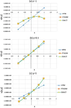
Fig. 2 and Fig. 3 show a comparison between the results of HPM, FTADM and exact values of the linear and non-linear NWS equations, respectively for only the first six recursive terms. The plots show that the behavior of FTADM values is very close to the exact values in comparison to the HPM results. This is even more pronounced for the non-linear NWS equation (Fig. 3).

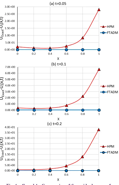
In Fig. 4, the residual errors of HPM and FTADM with respect to exact values of the non-linear NWS equation are compared for only the first six recursive terms. The figure

shows that the residual error of FTADM is much smaller than HPM results and the behavior of FTADM values is much closer to the exact values in comparison to the HPM results. The errors of HPM and FTADM with respect to the exact values of the NWS equation are plotted in Table 4. The root mean square (RMS) error of the results for

recursive terms are presented for HPM and FTADM. The RMS error for the first six recursive terms of HPM is much bigger than that of FTADM. This means that the FTADM has a much faster convergence rate towards the exact values than the HPM. This, in fact, shows the effectiveness of the FTADM in handling the nonlinear differential equations in comparison with the HPM.

Figs. 5 and 6 show the comparison of the results of HPM, FTADM and exact values of the linear and non-linear NWS equations respectively for only the first six recursive terms. The results show that as time grows, the values of FTADM converges to zero monotonically, for the linear NWS equation, and converges to 1, for the non-linear NWS equation. This is in agreement with the basic concept of NWS diffusion equation. This does not occur for the results of HPM as time increases. 5- Conclusion

In this work, the exact solutions to linear and non-linear NWS diffusion equations are obtained through the FTADM and HPM. The effectiveness and credibility of the FTADM are shown in comparison to HPM by solving three examples with linear and non-linear differential equations. The results of the series solution obtained by FTADM and HPM are compared Table 3. Comparison of relative error of and of

the HPM and FTADM results of example 3 (nonlinear NWS equation) at different x-coordinates and at different times

2

2( , )=

∑

i=₀ i( , ),

s x t u x t 4

4 ₀

( , )

s x t

=

∑

_i₌

u x t

_i

( , ),

6

6 ₀

( , )

s x t

=

∑

_i₌

u x t

_i

( , )

6

6 ₀

( , )

s x t

=

∑

_i₌

u x t

_i

( , )

2

2( , )=

∑

i=0 i( , ),

s x t u x t 4

4 0

( , )s x t =

∑

_i₌u x t_i( , ) 6

6 0

( , )s x t =

∑

_i₌u x t_i( , )

x=0 x=0.2 x=0.4 x=0.6 x=0.8 x=1

t=0.05

S4(x,t) HPM 2.061E-01 1.268E-01 1.123E-01 2.361E-01 7.476E-01 2.338E+00 FTADM 7.528E-06 2.286E-06 5.232E-06 1.379E-05 2.168E-05 2.721E-05

S6(x,t) HPM 2.061E-01 1.268E-01 1.135E-01 2.484E-01 8.376E-01 2.801E+00 FTADM 4.967E-08 1.304E-08 9.077E-08 1.560E-07 1.822E-07 1.554E-07

t=0.1

S4(x,t) HPM 3.398E-01 2.496E-01 3.177E-01 7.169E-01 1.950E+00 5.299E+00 FTADM 2.215E-04 9.473E-05 8.975E-05 3.009E-04 4.973E-04 6.380E-04

S6(x,t) HPM 3.398E-01 2.497E-01 3.217E-01 7.637E-01 2.245E+00 6.621E+00 FTADM 6.025E-06 1.644E-07 7.982E-06 1.470E-05 1.771E-05 1.566E-05

t=0.2

S2(x,t) HPM 9.236E-01 8.306E-01 1.125E+00 1.778E+00 2.764E+00 4.029E+00 FTADM 5.249E-02 4.580E-02 3.304E-02 1.458E-02 8.640E-03 3.530E-02

S4(x,t) HPM 9.236E-01 8.960E-01 1.595E+00 3.756E+00 9.082E+00 2.126E+01 FTADM 5.981E-03 3.544E-03 1.338E-04 4.399E-03 8.419E-03 1.141E-02

(9)

with the real exact solution. For the same number of terms in the series solutions, the error of the FTADM results is much smaller than those obtained by HPM. However, this is more pronounced for the case of the non-linear differential equation. Moreover, as time increases, i.e. t→∞, the results of FTADM, for the linear NWS equation, converges to zero and for, the non-linear NWS equation, the results of FTADM converges to 1 with only six recursive terms. However, this is not the case for the results of HPM. It can be deduced that the FTADM is an efficient and powerful tool which can yield the exact solution of linear and non-linear differential NWS equations more effective than HPM.

Fig. 1a, 1b and 1c. comparison of variations of with the exact values u(x,y) for example 1 using HPM and FTADM at (a) y=-1, (b) y=0.1, (c) y=1

6

6 0

( , )s x y =

∑

_i₌u x y_i( , )

Fig. 2a, 2b and 2c. comparison of variations of with the exact values u(x,t) for example 2 (linear NWS equation) using the HPM and FTADM

at (a) t=0.05, (b) t=0.1, (c) t=0.2

6

6 0

( , )

s x t

=

∑

_i₌

u x t

_i

( , )

t=0.05 t=0.1 t=0.2 RMS error of the

HPM method 1.20E+00 2.88E+00 1.64E+01 RMS error of the

FTADM method 1.24E-07 1.21E-05 9.47E-04 Table 4. Comparison of RMS error of

of the HPM

and FTADM results of example 3 (nonlinear NWS Equation) at different times .

6

6 0

( , )

s x t

=

∑

_i₌

u x t

_i

( , )

Fig 5. Behavior of

for the results of HPM and FTADM of example 2

(linear NWS equation).

6

6 ₀

(10)

REFERENCES

[1] J.-H. He, Application of homotopy perturbation method to nonlinear wave equations, Chaos, Solitons & Fractals, 26(3) (2005) 695-700.

[2] J.-H. He, Homotopy perturbation method for bifurcation of nonlinear problems, International Journal of Nonlinear

Sciences and Numerical Simulation, 6(2) (2005) 207-208. [3] J.-H. He, Homotopy perturbation method for solving

boundary value problems, Physics letters A, 350(1) (2006) 87-88.

[4] A.-M. Wazwaz, Partial differential equations and solitary waves theory, Springer Science & Business Media, 2010. [5] A. Yildirim, Homotopy perturbation method for the

mixed Volterra–Fredholm integral equations, Chaos, Solitons & Fractals, 42(5) (2009) 2760-2764.

[6] S.S. Nourazar, M. Soori, A. Nazari-Golshan, On the exact solution of Newell-Whitehead-Segel equation using the homotopy perturbation method, arXiv preprint arXiv:1502.08016, (2015).

[7] M.M. Rashidi, H. Shahmohamadi, Analytical solution of three-dimensional Navier–Stokes equations for the flow near an infinite rotating disk, Communications in Nonlinear Science and Numerical Simulation, 14(7) (2009) 2999-3006.

[8] O.A. Bég, M. Rashidi, T.A. Bég, M. Asadi, Homotopy analysis of transient magneto-bio-fluid dynamics of micropolar squeeze film in a porous medium: a model for magneto-bio-rheological lubrication, Journal of Fig 6. Behavior of

for the results of HPM and FTADM of example 3 (nonlinear NWS equation).

6

6 0

( , )

s x t

=

∑

_i₌

u x t

_i

( , )

Fig. 3a, 3b and 3c. comparison of variations of with the exact values u(x,t) for example 3 (nonlinear NWS equation) using HPM and FTADM

at (a) t=0.05, (b) t=0.1, (c) t=0.2.

6

6 0

( , )=

∑

₌ _i( , )

i

s x t u x t

Fig. 4a, 4b and 4c. Comparsion of the residual errors of of the HPM and FTADM results of example 3 (nonlinear NWS Equation) at (a) t=0.05,

(b) t=0.1, (c) t=0.2.

6

6 0

(11)

Mechanics in Medicine and Biology, 12(03) (2012) 1250051.

[9] M.H. Abolbashari, N. Freidoonimehr, F. Nazari, M.M. Rashidi, Entropy analysis for an unsteady MHD flow past a stretching permeable surface in nano-fluid, Powder Technology, 267 (2014) 256-267.

[10] S. Nourazar, A. Nazari-Golshan, A. Yıldırım, M. Nourazar, On the hybrid of Fourier transform and Adomian decomposition method for the solution of nonlinear Cauchy problems of the reaction-diffusion equation, Zeitschrift für Naturforschung A, 67(6-7) (2012) 355-362.

[11] A. Nazari-Golshan, S. Nourazar, H. Ghafoori-Fard, A. Yildirim, A. Campo, A modified homotopy perturbation method coupled with the Fourier transform for nonlinear and singular Lane–Emden equations, Applied Mathematics Letters, 26(10) (2013) 1018-1025.

[12] A. Saravanan, N. Magesh, A comparison between the reduced differential transform method and the Adomian decomposition method for the Newell–Whitehead–Segel equation, Journal of the Egyptian Mathematical Society, 21(3) (2013) 259-265.

[13] G. Adomian, Solving Frontier Problems of Physics: The Decomposition MethodKluwer, Boston, MA, (1994). [14] A.-M. Wazwaz, M.S. Mehanna, The combined

Laplace-Adomian method for handling singular integral equation of heat transfer, International Journal of Nonlinear Science, 10(2) (2010) 248-252.

[15] R.G. Pratt, C. Shin, G. Hick, Gauss–Newton and full Newton methods in frequency–space seismic waveform inversion, Geophysical Journal International, 133(2) (1998) 341-362.

[16] R.G. Pratt, M. Worthington, Inverse theory applied to multi-source cross-hole tomography. Part 1: Acoustic wave-equation method, Geophysical prospecting, 38(3) (1990) 287-310.

[17] T. Wu, Z. Chen, A dispersion minimizing subgridding finite difference scheme for the Helmholtz equation with PML, Journal of Computational and Applied Mathematics, 267 (2014) 82-95.

Please cite this article using:

S. S. Nourazar, H. Parsa, A. Sanjari, A Comparison Between Fourier Transform Adomian Decomposition Method and Homotopy Perturbation Method for Linear and Non-Linear Newell-Whitehead-Segel Equations, AUT J. Model. Simul., 49(2)(2017)227-238.

(12)