The Sectional Stratospheric Sulfate Aerosol module (S3A-v1) within
the LMDZ general circulation model: description and evaluation
against stratospheric aerosol observations
Christoph Kleinschmitt1,2, Olivier Boucher3, Slimane Bekki4, François Lott5, and Ulrich Platt1
1Institute of Environmental Physics, Heidelberg University, Im Neuenheimer Feld 229, 69120 Heidelberg, Germany 2Laboratoire de Météorologie Dynamique, Institut Pierre-Simon Laplace, CNRS/UPMC, 4 place Jussieu, 75252 Paris CEDEX 05, France
3Institut Pierre-Simon Laplace, CNRS/UPMC, 4 place Jussieu, 75252 Paris CEDEX 05, France
4Laboratoire Atmosphères Milieux Observations Spatiales, Institut Pierre-Simon Laplace, CNRS/UVSQ, 11 boulevard d’Alembert, 78280 Guyancourt, France
5Laboratoire de Météorologie Dynamique, Institut Pierre-Simon Laplace, CNRS/ENS, 24 rue Lhomond, 75231 Paris CEDEX 05, France
Correspondence to:Christoph Kleinschmitt ([email protected]) Received: 3 February 2017 – Discussion started: 5 April 2017
Revised: 2 August 2017 – Accepted: 8 August 2017 – Published: 12 September 2017
Abstract. Stratospheric aerosols play an important role in the climate system by affecting the Earth’s radiative budget as well as atmospheric chemistry, and the capabilities to sim-ulate them interactively within global models are continu-ously improving. It is important to represent accurately both aerosol microphysical and atmospheric dynamical processes because together they affect the size distribution and the res-idence time of the aerosol particles in the stratosphere. The newly developed LMDZ-S3A model presented in this article uses a sectional approach for sulfate particles in the strato-sphere and includes the relevant microphysical processes. It allows full interaction between aerosol radiative effects (e.g. radiative heating) and atmospheric dynamics, including e.g. an internally generated quasi-biennial oscillation (QBO) in the stratosphere. Sulfur chemistry is semi-prescribed via climatological lifetimes. LMDZ-S3A reasonably reproduces aerosol observations in periods of low (background) and high (volcanic) stratospheric sulfate loading, but tends to overes-timate the number of small particles and to underesoveres-timate the number of large particles. Thus, it may serve as a tool to study the climate impacts of volcanic eruptions, as well as the deliberate anthropogenic injection of aerosols into the stratosphere, which has been proposed as a method of geo-engineering to abate global warming.
1 Introduction
rel-atively high resolution in aerosol size but only one dimension (i.e. height) in space.
An accurate representation of dynamical processes in the stratosphere (e.g. subtropical meridional transport bar-riers, Brewer–Dobson circulation, stratosphere–troposphere exchange) is also paramount to properly simulate the distri-bution of stratospheric aerosols and their dispersion follow-ing volcanic eruptions. Representfollow-ing accurately the interplay between aerosol microphysical and dynamical processes can be presumed to be computationally very expensive as it in-volves at least five dimensions: three space dimensions, the aerosol size dimension, and the time dimension. This means that, for a given computational cost, some trade-off is nec-essary between the representation (or discretisation) of these dimensions and/or the length of the simulation and the num-ber of simulations. One possibility is to exploit the approx-imately zonal symmetry in the stratosphere to reduce the atmosphere to the height and latitude dimensions. This ap-proach was used in particular by Bekki and Pyle (1992) and Mills et al. (1999), who retained the sectional approach to represent aerosol size.
The increase in computational capability has progressively allowed the development of three-dimensional models of stratospheric aerosols in the late 1990s/early 2000s. Most of these models were initially chemistry-transport models (CTMs). This so-called offline approach was often preferred because chemistry-transport models are cheaper to run as wind and temperature fields are specified according to me-teorological analyses instead of being calculated prognos-tically like in climate-chemistry models. In addition, since the transport of tracers is driven by meteorological analyses, the observed day-to-day variability in chemical composition can be reproduced (at least to some extent), facilitating the comparisons with measurements. While chemistry-transport models are suitable for a broad range of studies, they do not include any radiative feedback between chemical composi-tion and dynamics, and notably ignore the radiative effects of aerosols on atmospheric dynamics.
Given the importance of stratospheric aerosols for the Earth’s radiative budget, there is also a need to repre-sent stratospheric aerosols in climate models. The volcanic aerosol forcing is important to simulate the temporal evolu-tion of the climate system over the last millennium in gen-eral, and over the instrumental period (1850 to the present day) in particular. This was initially done by prescribing the amount and properties of stratospheric aerosols as (time-varying) climatologies derived from observations. This was the case in most if not all of the climate models involved in the fifth phase of the Climate Model Intercomparison Project (CMIP5) as discussed in Flato et al. (2013), and it is still expected to be the case in the forthcoming sixth phase (CMIP6) (Eyring et al., 2016). However, capabilities to sim-ulate stratospheric aerosols within global climate models are continuously improving.
The SPARC stratospheric aerosol assessment report (Thomason and Peter, 2006) provides a review of strato-spheric aerosol models as of 10 years ago. It clearly repre-sents a milestone and stimulated significant further model development since then. As a result, the recent review by Kremser et al. (2016) lists more than a dozen global three-dimensional stratospheric aerosol models. It should be noted however that several of these configurations share the same atmospheric general circulation model (GCM) or the same aerosol module, and not all of them include the interaction of aerosols with radiation.
The sectional approach has been adopted by a number of these three-dimensional stratospheric aerosols (e.g. Timm-reck, 2001; Pitari et al., 2002; Sheng et al., 2015). Strato-spheric aerosols have also been modelled in climate mod-els as an extension of schemes initially designed for tro-pospheric aerosols. Simple mass-based (i.e. bulk) aerosol schemes modified to account for gravitational settling of the sulfate aerosols have been used occasionally (Oman et al., 2006; Haywood et al., 2010; Aquila et al., 2012). Such mod-els do not represent the growth of aerosol particles, but rely instead on a fixed size distribution for each aerosol type. More sophisticated approaches have also been developed, whereby the aerosol size distribution is approximated by a statistical function with a pre-defined shape and a few vari-able parameters. The evolution of the size distribution is gov-erned through variations in these selected parameters but, by construction, it has only a few degrees of freedom, which may lead to discrepancies and artefacts in the simulated size distribution. Examples include two-moment modal aerosol microphysics schemes such as the M7 model (Vignati et al., 2004; Stier et al., 2005) and the GLOMAP model (Mann et al., 2010; Dhomse et al., 2014), whereby each aerosol mode is represented prognostically by a number and a mass concentration.
large cost of the sectional approach may limit the horizontal or vertical resolutions of the atmospheric model.
A climate model with a well-established stratospheric aerosol capability is the WACCM/CARMA model described by English et al. (2011) (for WACCM, see Garcia et al., 2007, and for CARMA, see Toon et al., 1988) which includes a sectional stratospheric aerosol with all the relevant chem-istry and microphysics, along with a high vertical resolution. However, the model does not consider aerosol radiative heat-ing. Recently Mills et al. (2016) used the WACCM model to simulate the time evolution of the stratospheric aerosol over the period 1990–2014. They find a good agreement in strato-spheric aerosol optical depth (SAOD) with SAOD derived from several available lidar measurements by Ridley et al. (2014) and in surface area density (SAD) with balloon-borne optical particle counter (OPC) measurements at the Univer-sity of Wyoming (Kovilakam and Deshler, 2015).
Our research on stratospheric aerosols is motivated by their interaction with both incoming solar radiation and out-going terrestrial radiation, and the associated climate re-sponse to such a radiative forcing. We are interested in a wide range of stratospheric aerosol burdens: from background lev-els to the large volcanic loads observed after major erup-tions such as El Chichón, Pinatubo (e.g. Dutton and Christy, 1992), Krakatoa, or Tambora. Furthermore, we are inter-ested in studying the potential of stratospheric aerosol injec-tion (SAI) as a geoengineering means to artificially cool the Earth’s climate in order to compensate for greenhouse gas global warming (e.g. Budyko, 1977; Crutzen, 2006). Recent reviews of scientific studies and open questions regarding so-lar geoengineering (e.g. Irvine et al., 2016; MacMartin et al., 2016) highlighted again the need for accurate stratospheric aerosol models. These research interests motivate the intro-duction of a versatile stratospheric aerosol model within the IPSL Climate Model (IPSL-CM) and its atmospheric compo-nent LMDZ. As a first step towards this objective we have in-troduced a sectional stratospheric sulfate aerosol model in the LMDZ model. We have included processes relevant to both the background and volcanic stratospheric aerosol layer, but also processes relevant to much larger and/or longer emission rates than experienced in typical volcanic eruptions.
In this article we offer a full and detailed description of the aerosol model in Sect. 2. We also evaluate its perfor-mance against available observations. The eruption of Mount Pinatubo in June 1991 is the last major eruption experienced by the Earth and was relatively well observed. As such it is a useful case study for any stratospheric aerosol model and is discussed in Sect. 3.
can be coupled to the ORCHIDEE land surface model (Krin-ner et al., 2005), the oceanic GCM NEMO (Madec, 2008) and other biogeochemical or chemical model components to form the IPSL Earth system model (Dufresne et al., 2013). It is thus possible to use the S3A model to study the climate response to volcanic eruptions or SAI. We briefly describe below the host atmospheric model in Sect. 2.1 and make a comprehensive description of the S3A model in Sect. 2.2. 2.1 Host atmospheric model
2.1.1 Model resolution and model physics
A full description of the LMDZ model in its LMDZ5A con-figuration is available in Hourdin et al. (2006) and Hourdin et al. (2013). We do not repeat the description here but in-stead focus on the evolutions of the model since Hourdin et al. (2013) and the specificities of the LMDZ configuration considered in this study.
In the configuration tested here with the S3A module, LMDZ is run with 96×96 grid points, i.e. a horizontal res-olution of 1.89◦in latitude and 3.75◦ in longitude – which is the same as for LMDZ5A –, but with a vertical resolution increased to 79 layers and a model top height of 75 km. The additional layers are mostly located in the stratosphere so that in the lower stratosphere (between 100 and 10 hPa) the ver-tical spacing1zis approximately 1 km in this model set-up. The increased resolution on the vertical aims to “close” the stratospheric circulation. It is also necessary to generate a re-alistic quasi-biennial oscillation (QBO) as discussed below. de la Cámara et al. (2016) provide a more extensive descrip-tion of the stratospheric dynamics modelled with this verti-cally enhanced configuration of LMDZ.
Our configuration of the LMDZ model differs from that described in Hourdin et al. (2013) in that it has a different radiative transfer code. In the shortwave, the code is an ex-tension to six bands of the initial two-band code that is used in LMDZ5A (Fouquart and Bonnel, 1980), as implemented in a previous version of the ECMWF numerical weather pre-diction model. In the longwave, we use the ECMWF imple-mentation of the RRTM radiative transfer scheme (Mlawer et al., 1997) with 16 spectral bands. This change in radiative transfer scheme is motivated by the necessity to account for the radiative effects of the stratospheric aerosols in both the shortwave (SW) and longwave (LW) parts of the spectrum with sufficient spectral resolution.
2.1.2 Tropopause recognition
As the model focuses on stratospheric aerosols, the separa-tion between troposphere and stratosphere (i.e. the locasepara-tion of the tropopause) is of special importance. The S3A model requires the knowledge of whether a particular model grid box is located in the troposphere or the stratosphere, be-cause the processes of nucleation, condensation, evaporation, and coagulation are only activated in the stratosphere. Tro-pospheric aerosols are treated separately by a standard bulk aerosol model (e.g. Escribano et al., 2016). Also, we have a set of stratospheric aerosol variables that are only diagnosed in the stratosphere.
To this effect we use the algorithm by Reichler et al. (2003) which is based on the WMO definition of the tropopause as “the lowest level at which the lapse-rate decreases to 2 K km−1 or less, provided that the average lapse-rate be-tween this level and all higher levels within 2 km does not exceed 2 K km−1”. We use the FORTRAN code provided by Reichler et al. (2003), which we have adapted to the LMDZ model. With this the tropopause pressure is computed at each timestep. In the rare case that the algorithm does not find the tropopause in a grid column, it is set to a default value that only depends on the latitudeϕ(in radians) through the rela-tionship
pTP[hPa] =500−200·cos(ϕ). (1)
In this case the tropopause is assumed to vary between 300 hPa at the Equator and 500 hPa at the Poles, indepen-dently of the season.
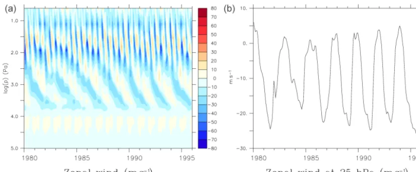
2.1.3 Quasi-biennial oscillation in the stratosphere The vertical extension to the LMDZ domain, as discussed above, is accompanied by a new stochastic parametrisation of gravity waves produced by convection which is documented in Lott and Guez (2013). This is another difference to the original LMDZ5A model configuration described in Hour-din et al. (2013) which did not include this parametrisation. The combination of the extended vertical resolution in the lower stratosphere and the gravity wave parametrisation gen-erates a QBO in the model, as shown in Fig. 1 and docu-mented in Lott and Guez (2013). The amplitude of the QBO around 10 hPa is around 10–15 m s−1and is smaller than ob-served (20–25 m s−1). The easterly phases are also stronger and longer in duration than the westerly phases, which is re-alistic. One subtle difference with the QBO shown in Lott and Guez (2013) is that here the connection with the semi-annual oscillation (SAO) above is quite pronounced, whereas it was not so evident in Lott and Guez (2013). This is because the characteristic phase speed we have recently adopted for the convective gravity wavesCmax=30 m s−1(de la Cámara et al., 2016) is smaller than for the convective gravity wave parameter we used in Lott and Guez (2013). The stronger connection can be further explained by the fact that more
waves travelling through the QBO sector will likely be ab-sorbed by the critical levels produced by the SAO. Finally, it is worthwhile recalling that our QBO does not extend down to 100 hPa, in contradiction with observations. In our model, it is probably due to the fact that we underestimate the ex-plicit slow Kelvin waves that play a crucial role in the lower stratosphere (Giorgetta et al., 2006; for the Kelvin waves in models, see Lott et al., 2014).
It is noticeable that the period of our simulated QBO in Fig. 1 shortens and its amplitude increases during the sec-ond half of the simulation, e.g. as the aerosol layer builds up in the lower stratosphere. More precisely, the QBO has a period well above 26 months during the first 5 years be-fore evolving to an almost purely biennial oscillation by the end of the simulation. This could be due to the warming of the stratosphere induced by the developing stratospheric aerosol layer (up to 1.5 K in the tropical lower stratosphere), which would be consistent with the opposite behaviour found when the stratosphere cools, e.g. in response to an increase in greenhouse gases (for the intensity and period, see de la Cámara et al., 2016; for intensity only, see the observations in Kawatani and Hamilton, 2013). As our simulation is quite short, this result should be consolidated by longer runs. It should also be kept in mind that since the QBO in our model is probably oversensitive to changes in greenhouse gases, it may also be oversensitive to the aerosol content.
Despite these shortcomings, the self-generated QBO is an attractive feature of the LMDZ model to study stratospheric aerosols and different SAI scenarios. A more realistic simu-lation of the QBO would require a higher horizontal resolu-tion.
2.1.4 Nudging to meteorological reanalysis
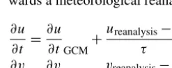
As an option, the LMDZ model can be nudged to a meteo-rological reanalysis. This is useful for simulating a historical situation with particular meteorological conditions. Only the horizontal wind componentsu andv are nudged. Nudging is performed by adding an additional term to the governing differential equations foruandvwhich relaxes the wind to-wards a meteorological reanalysis:
∂u ∂t =
∂u ∂tGCM
+ureanalysis−u
τ ;
∂v ∂t =
∂v ∂tGCM
+vreanalysis−v
τ ; (2)
Figure 1. (a) Altitude–time profile of the zonal wind (in m s−1), averaged between 10◦S and 10◦N, from a simulation with evolving background aerosol. The vertical axis shows the logarithm of the pressure in Pa.(b)Zonal wind at 25 hPa, averaged between 10◦S and 10◦N.
2.2 The sectional stratospheric sulfate aerosol (S3A) model
2.2.1 Prognostic variables
The S3A module in the configuration introduced here repre-sents the stratospheric aerosol size distribution with NB= 36 size bins of sulfate particles, with a dry radius rang-ing from 1 nm to 3.3 µm (i.e. r1=1 nm and rN=3.3 µm for particles at 293 K consisting of 100 % H2SO4) and par-ticle volume doubling between successive bins (i.e. RV =
Vk+1/Vk=rk3+1/r 3
k =2 for 1≤ k < NB). The number of size binsNBand the corresponding value ofRV represent a compromise between the accuracy of the scheme, which in-creases with higher resolution in size, and the computational cost of the model.
It should be noted that therk are the radii of the “middle” of the size bins. The radii of the lower and upper boundaries of binkare
rklower=
rk/ r
R 1 3
V fork=1 √
rk−1rk for 1< k≤NB
;
rkupper=
√
rkrk+1 for 1≤k < NB
rk· r
R 1 3
V fork=NB
. (3)
Other global stratospheric models with sectional aerosol schemes have resolutions ranging from 11 to 45 size bins (Thomason and Peter, 2006). Our model resolution of 36 size bins is therefore on the high end of this range. A relatively high size resolution is required for an accurate modelling of stratospheric aerosols because coagulation, an important pro-cess in the stratosphere, and gravitational sedimentation, the
main loss process in the stratosphere, are very strongly de-pendent on the aerosol size.
The lower end of our size range (1 nm) was chosen to be close to the size of typical freshly nucleated particles. We have tried to limit the number of bins by increasing the minimum aerosol size to 10 nm or more and feeding the nucleation term directly into this bin. However, this re-sulted in inaccuracies in the size distribution at both small and large aerosol sizes, so this simplification was eventually not adopted. Large particles have short residence times and therefore very low concentrations in the stratosphere. As a re-sult they do not contribute much to the aerosol optical depth; hence, it is acceptable to set an upper range to 3.3 µm for our modelled size distribution. While 36 size bins correspond to our current configuration, the size range and size resolution can easily be changed in our model by adjusting the num-ber of size bins (NB), the minimum dry aerosol size (r1), and the volume ratio between bins (RV). All the parametrisations described below then adjust to the new size discretisation.
Aerosol amount in each of the size bins is treated as a sep-arate tracer for atmospheric transport in the unit of particle number per unit mass of air as required by our mass-flux scheme (Hourdin and Armengaud, 1999).
2.2.2 Semi-prognostic sulfur chemistry
deposi-tion, and chemical transformations. The chemical reactions transforming one species to another (OCS into SO2and SO2 into H2SO4) during one model timestep are parametrised as exponential decay terms with prescribed chemical lifetimes:
1[SO2] = M(SO2)
M(OCS)· [OCS] ·
1−exp
−1tphys τOCS
, (4)
1[H2SO4] =M(H2SO4) M(SO2)
· [SO2] ·
1−exp
−1tphys
τSO2
, (5)
with[X]being the mixing ratio,1[X]the change in mixing ratio, M(X)the molecular mass, andτX the chemical life-time of speciesX.
Both the climatological values of OCS and SO2and their chemical lifetimes are taken from a latitude–altitude clima-tology at monthly resolution from the UPMC/Cambridge global two-dimensional chemistry-aerosol-transport model (Bekki and Pyle, 1992, 1993). These quantities are shown in Fig. 2. Using prescribed chemical lifetimes means that the OCS and SO2concentrations do not feed back onto concen-trations of oxidants which oxidise these species. This is a limitation of our model, especially in case of large OCS or SO2injection rates, which we discuss further in Sect. 3.3.2. In a future study the S3A model will be coupled to the REPROBUS (Reactive Processes Ruling the Ozone Budget in the Stratosphere) model for stratospheric chemistry that is also available in the LMDZ model (Lefèvre et al., 1994, 1998).
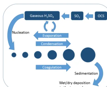
A schematic of the model species and physical processes is shown in Fig. 3. The following processes are represented: aerosol nucleation from gaseous H2SO4, condensation and evaporation of gaseous H2SO4, coagulation, and sedimenta-tion of aerosol particles. Dry and wet deposisedimenta-tion of gas-phase species and aerosols in the troposphere is also considered as we are interested in the tropospheric fate of the stratospheric aerosols.
2.2.3 Nucleation
The formation rate of new particles via binary homogeneous nucleation of sulfuric acid and water vapour is parametrised as a function of the sulfuric acid gas-phase concentration, the relative humidity, and the absolute temperature as de-scribed by Vehkamäki et al. (2002). This parametrisation pro-vides the nucleation rateJnuc in units of particles cm−3s−1, the total number of molecules in each nucleated particle
Ntot, and the mole fraction of H2SO4in the new particlex. The equations are cumbersome and not repeated here, but it should be noted that we rely on the Fortran code provided by Vehkamäki et al. (2002).
The parametrisation is not valid any more under condi-tions where the number of molecules in the critical clus-ter is below 4 (which occurs mainly at large H2SO4vapour
concentrations). Under such conditions, we take the colli-sion rate of two H2SO4molecules as the nucleation rate in-stead (H. Vehkamäki, personal communication, 2015), i.e.
Ntot=2,x=1, and
Jnuc(Ntot<4)=[H2SO4]2· 3π 4 16 · 12k BT
M(H2SO4)
12
·2V (H2SO4)
1 3
2
, (6)
with M(H2SO4) the molecular mass of sulfuric acid, [H2SO4] the concentration of H2SO4 (in molecules cm−3),
kB the Boltzmann constant, and V (H2SO4) the molecular volume of H2SO4 which is computed using Vehkamäki’s density parametrisation.
In order to sort the new particles into the model size bins in a mass-conserving way, their volume is computed as
Vnewnuc=M(H2SO4)Ntotx ρ(H2SO4)
(7) with the density of sulfuric acidρ(H2SO4)taken at the ref-erence temperature 293 K. The new particles are distributed among the size bins using a method inspired by the distri-bution factorfi,j,k from Jacobson et al. (1994) described in Sect. 2.2.6 and Eq. (19). Hereby for each new particle we add
fknuc·Vnewnuc/Vkparticles to bink, withVk=43π rk3and
fknuc= (8)
V k+1−Vnewnuc Vk+1−Vk
Vk Vnuc
new forVk
≤Vnewnuc< Vk+1; k < NB
1−fknuc−1 forVk−1≤Vnewnuc< Vk; k >1 1 for Vnewnuc≤Vk; k=1
or
Vnewnuc≥Vk; k=NB
0 otherwise.
As a result the actual particle nucleation rate may deviate from Vehkamäki’s parametrised value. For example, if the nucleated particles have only half the volume of a particle in the smallest model size bin, the number of new particles is only half of the parametrised value, but the H2SO4 flux from the gas to the particle phase is the same. We favoured conserving sulfur mass over conserving particle number con-centration. This approximation of the exact value of the nu-cleation rate is not expected to have a very significant impact on the results because the particle size distribution is mainly determined by coagulation and condensation (English et al., 2011). Furthermore, this approximation is justified in the light of the large uncertainties arising from parametrising nu-cleation rates using grid-box quantities (temperature, H2O, H2SO4) that neglect sub-grid-scale variations.
Figure 2.Climatological volume mixing ratios (upper half, in pptv) and lifetimes (lower half, in years or days) of OCS and SO2produced by the UPMC/Cambridge model and used as initial and boundary conditions for the LMDZ-S3A model. The left column shows the zonal and annual mean latitude–height distribution, while the right column shows an annual cycle of the zonal mean value at 20 km altitude.
on the UPMC/Cambridge model parametrisation (Bekki and Pyle, 1992, 1993).
First the saturation vapour pressure of H2SO4 over a flat surface is calculated from a relationship given by Ayers et al. (1980) using the values of H2SO4chemical po-tentials in aqueous phase listed in the work of Giauque et al. (1960, Table I):
psatH
2SO4[Pa] =
101325 0.086
·exp
−10156
T +16.259+ µ−µ0
RT
, (9)
with T the temperature, µ the chemical potential, and
Figure 3. Schematic representation of the sulfur species and the processes affecting them that are represented in the LMDZ-S3A model.
We account for the Kelvin effect, whereby the saturation vapour pressure of H2SO4 over a curved surface is higher than the saturation vapour pressure over a flat surface. The saturation vapour pressure over a sulfate aerosol particle in size bink, with radiusrk, is
psatH,k 2SO4=p
sat H2SO4·exp
2σ M(H 2O)
ρpkBT rk
, (10)
withM(H2O)the molecular mass of water,σthe surface ten-sion of the sulfuric acid solution (which is set to 72 mN m−1, the value for water at 20◦C), andρpthe density of the sul-fate particles. The corresponding H2SO4 number density at saturation is then
[H2SO4]sat,k=p
sat,k H2SO4 kBT
. (11)
Then the flux of H2SO4between the particle and the gas phase,Jk(H2SO4), in molecules particle−1s−1is computed individually for every size binkfollowing Seinfeld and Pan-dis (2006, pp. 542–547):
Jk(H2SO4)=π rk2v (H2SO4) α·
[H2SO4]−[H2SO4]sat,k
· 1+Knk
1+Knk+α/(2Knk)
, (12)
with the molecular accommodation coefficient α=0.1,
v(H2SO4) the thermal velocity of a H2SO4 molecule, and Knk=λ/rk the Knudsen number, where we use the parametrisation from Pruppacher and Klett (2010, p. 417) for the mean free path of air
λ=λ0· p 0 p · T T0 (13)
with λ0=6.6·10−8m for air at standard conditions p0= 1013.25 hPa andT0=293.15 K.
Evaporation from a particle over one timestep is limited to its actual H2SO4content and condensation is limited by the available H2SO4vapour. How this is dealt with is further described in Sect. 2.2.5.
Condensation (evaporation) has an impact on the particle size distribution, shifting particles to larger (smaller) sizes. To account for this, we first compute the new particle volume after adding the fluxJk(H2SO4)over the timestep1t:
Vk,c/newe =Vk·
1+Jk(H2SO4)1t Nk(H2SO4)
, (14)
whereNk(H2SO4)is the number of sulfuric acid molecules in a particle for bink. Knowing this new volume of a particle coming from binkand experiencing condensation or evapo-ration, the distribution among all the size bins (indexl) can then be computed analogously to Eqs. (8) and (19) using a factor:
fk,lc/e= (15)
Vl+1−Vk,c/newe Vl+1−Vl
Vl
Vk,c/newe forVl
≤Vk,c/newe < Vl+1; l < NB
1−fk,lc/e−1 forVl−1≤Vk,c/newe < Vl; l >1 1 for hVk,c/newe ≤Vl ; l=1
i or h
Vk,c/newe ≥Vl; l=NB i
0 otherwise.
2.2.5 Competition between nucleation and condensation
As both processes, nucleation and condensation, consume H2SO4vapour while having very different effects on the par-ticle size distribution, the competition between the two pro-cesses has to be handled carefully in a numerical model. Fur-thermore, this has to be done at an affordable numerical cost, as we aim to perform long global simulations. We address this in the S3A module using an adaptive sub-timestepping. After computing the H2SO4fluxes due to nucleation and con-densation in kg H2SO4s−1 from the initial H2SO4 mixing ratio, a sub-timestep, 1t1, is computed such that the sum of both the nucleation and condensation fluxes consumes no more than 25 % of the available ambient H2SO4vapour:
1t1=min
0.25· [H2SO4]0 Jnuc+Jcond
, 1tphys
, (16)
where1tphysis the main timestep (30 min in our case), and
[H2SO4]0is the H2SO4mixing ratio at the beginning of the timestep. Hence, neither one of the two processes can use up all the sulfuric acid at the expense of the other process. This sub-timestepping procedure is repeated up to four times with a sub-timestep equal to
1t1<i<4=min 0.25·
[H2SO4]0
Jnuc+Jcond
, 1tphys−
i−1 X
j=1
1tj
1t4=max "
min 0.25· [H2SO4]0 Jnuc+Jcond
, 1tphys− 3 X
j=1
1tj !
,
1tphys− 3 X
j=1
1tj #
(18)
This joint treatment of nucleation and condensation is im-perfect, but it has the advantage of being much more com-putationally efficient than the usual solutions consisting of taking very short timesteps and much simpler than a simul-taneous solving of nucleation and coagulation. The number of sub-timesteps could be increased for increased numerical accuracy; however, a number of four sub-timesteps was con-sidered to be sufficient. It should be noted that the processes of nucleation and condensation, as well as their competition, are only activated in the stratosphere.
2.2.6 Coagulation
The growing of sulfate particles through coagulation is rep-resented through the semi-implicit, volume-conserving nu-merical scheme described in Jacobson et al. (1994). It is un-conditionally stable even for timesteps of the order of hours. We restricted the coagulation kernel to its main component only, i.e. Brownian motion. Secondary components of coag-ulation due to convection, gravitation, turbulence, or inter-particle van der Waals forces are neglected, which may partly explain the underestimation of particle size in Sect. 3. Sensi-tivity studies performed by English et al. (2013) and Sekiya et al. (2016) simulating the 1991 eruption of Mount Pinatubo found that including inter-particle van der Waals forces in-creased the peak effective radius by 10 % and dein-creased stratospheric AOD and burden by 10 %. Given that there are only a few measurements to constrain the van der Waals co-agulation term, and the mixed results obtained in our model (see Sect. 3.3.1), we do not include this process in our de-fault model, but offer it as an option in the code of the model (using the enhancement factors from Eqs. 29 and 30 in Chan and Mozurkewich, 2001). Coagulation is only activated in the stratosphere.
For convenience, we repeat here the equations from Ja-cobson et al. (1994). New particles resulting from the coag-ulation of particles from size binsiandj have a combined particle volumeVi,j=Vi+Vj. They are distributed among the size bins according to the following definition of the dis-tribution factorfi,j,k:
0 otherwise.
As discussed previously, the same distribution factor is ap-plied for the other physical processes affecting particle size (i.e. nucleation and the net effect from condensation and evaporation). To our knowledge, this is an original feature of our model. It should be noted that we have favoured con-servation of aerosol mass (and volume) over concon-servation of aerosol number in all these processes.
The semi-implicit approach gives the following equation for the concentration of particles in bink after coagulation over a timestep1t:
VkC(tk+1)=
VkCk(t )+1t k
P
j=1
k−1 P
i=1
fi,j,kβi,jViC(t +1)
i C
(t ) j
!
1+1t
NB
P
j=1
1−fk,j,k
βk,jC(t )j
, (20)
withCk(t ) the particle concentration in bin k at timestep t,
Ck(t+1) the particle concentration in binkat timestep t+1, andβi,j the coagulation kernel. For purely Brownian coagu-lation, the kernel has the form
βi,jB = 4π ri+rj
Di+Dj ri+rj
ri+rj+
δ2 i+δ2j
1
2
+ 4(Di+Dj)
v2p,i+v2p,j(ri+rj)
(21)
with the particle diffusion coefficient
Di=
kBT 6π riη
1+Kni
1.249+0.42·exp
−0.87 Kni
(22) whereηis the dynamic viscosity of air, the thermal velocity of a particle in biniwith massmi
vp,i= s
8kBT
π mi
(23)
the mean distance from the centre of a sphere reached by particles leaving the surface of the sphere and travelling a distance of the particle mean free pathλp,i
δi=
2ri+λp,i 3
−4ri2+λ2p,i 3 2
6riλp,i
−2ri (24)
and the particle mean free path
λp,i= 8Di
π vp,i
2.2.7 Aerosol chemical composition and density The weight fraction of H2SO4in the aerosol as a function of temperature and H2O partial pressure is computed following the approach described in Steele and Hamill (1981) and also used in Tabazadeh et al. (1997). In this approach, the water content of the aerosol particles is assumed to be in equilib-rium with the surrounding ambient water vapour. The com-position is assumed to be constant over the whole particle size range.
The aerosol particle density as a function of temperature and H2SO4weight fractionwH2SO4 (in %) can then be
com-puted from the rough approximation
ρp=
A·w2H
2SO4+B·wH2SO4+C
·
1−0.02
30 (T−293)
(26) with the constants A=7.8681252·10−6, B=8.2185978·
10−3,C=0.97968381, andT in K. 2.2.8 Sedimentation
Particles in the stratosphere sediment due to gravity with a velocity depending on their size and density and ambient pressure. The Stokes sedimentation velocity (with Cunning-ham correction) of a particle in size binkis given by
vsed,k=
2grk2 ρp−ρair 9η
1+Knk
1.257+0.4
·exp −1.1
Knk
, (27)
with the gravity g, the particle densityρp, and the air density
ρair.
The sedimentation process is computed with a semi-implicit scheme as described in Tompkins (2005). The con-centration of particles in a bink(omitted here for clarity) in the model layerj (withj numbered from the top of the at-mosphere to the surface) after sedimentation at timestept+1 is given by
Cj(t+1)=
Cj(t )+Cj(t−+11)·ρj−1vj−1 ρj1zj 1tphys 1+ ρjvj
ρj1zj1tphys
, (28)
with vj the sedimentation velocity, ρj the air density, and
1zj the thickness of layer j. The scheme is solved down-wards, it is very stable, and a timestep1tphysof 30 min is ap-propriate for our model vertical resolution. Unlike the aerosol processes described above, it is active not only above but also below the tropopause. It is applied to all bins of the aerosol size distribution, but has a noticeable impact only on larger particle bins.
Once the particles cross the tropopause they are rapidly re-moved from the troposphere through wet and dry deposition.
Parametrisations of dry and wet scavenging are those of the LMDZ model and are not described here as they have mini-mal impact on the stratospheric aerosol layer. They are never-theless important for modelling the tropospheric fate and im-pact at the surface of aerosols or aerosol precursors injected into the stratosphere.
2.3 Aerosol optical properties
Averaged optical properties of the particles (extinction cross section σi in m2 per particle in bin i, asymmetry param-eter gi, and single scattering albedoωi) are computed for each of the 6 SW and 16 LW spectral bands of the radia-tive transfer scheme using refracradia-tive index data from Hum-mel et al. (1988). We use our own Mie routine derived from Wiscombe (1979) and widely tested by the authors. In the SW, we account for variations of the incoming solar radia-tion within each band by computing aerosol optical proper-ties at a higher spectral resolution (24 spectral bands) and weighting the properties with a typical solar spectrum. In the LW, we account for variations in the refractive index of the aerosols within each band by computing aerosol optical erties at a higher spectral resolution and weighting the prop-erties with a black body emission spectrum using a typical stratospheric temperature of 220 K. To avoid Mie resonance peaks in the aerosol optical properties, we subdivide each aerosol size bin into 10 intervals which are logarithmically spaced and assume a uniform distribution within the size bin for computing average properties. For very small Mie param-eters (x <0.001), which occurs for the smallest particle bins and the longest wavelengths in the infrared, we extrapolate the Mie properties computed for x=0.001 for numerical stability using known asymptotic behaviour of the scatter-ing and absorption properties. Aerosol optical properties are computed once for each aerosol bin assuming a constant sul-furic acid mass mixing ratio of 75 % and a temperature of 293 K (conditions for which the refractive index was mea-sured) and are then integrated over the size distribution at every timestep according to the actual local size distribution. Hence, the optical depthτk, the single scattering albedoωk, and the asymmetry parametergkin model layerkwith parti-cle concentrationsCi,k(in particles per m3) and the vertical extent1zk (in m) can be computed as
τk= NB X
i=1
σiCi,k1zk; ωk= 1
τk NB X
i=1
ωiσiCi,k1zk;
gk= 1
τkωk NB X
i=1
giωiσiCi,k1zk. (29)
Figure 4. (a)Annual mean latitude–longitude distribution of the stratospheric AOD at 550 nm.(b)Zonal mean latitude–time distribution of the stratospheric AOD at 550 nm.(c)Zonal mean latitude–height distribution of the stratospheric aerosol extinction coefficient (km−1) at 550 nm.(d)Mass size distribution at different latitudes (in kg m−2). All variables are from the 10th year of the simulation with no volcanic input in the stratosphere and are assumed to represent a steady state.
3 Model validation
3.1 Non-volcanic background aerosol
The capability of our model to simulate a reasonable back-ground stratospheric sulfate aerosol is tested by running the model for a decade with climatological monthly and zonal mean OCS and SO2concentrations and lifetimes (shown in Fig. 2) as the only boundary conditions. In this set-up the model is not nudged to meteorological reanalysis.
The self-evolving aerosol distribution reaches a steady state or equilibrium (subject to seasonal variations) after about 5 years. In this steady state the global mean strato-spheric aerosol optical depth (SAOD) at 550 nm is 0.002, which is in good agreement with the observed SAOD of
0.002–0.0025 at 525 nm (in the tropics and at mid-latitudes) during the period of very low stratospheric sulfur loading around the year 2000 (e.g. Vernier et al., 2011). The global stratospheric aerosol burden is 0.08 Tg S and the mean dry ef-fective radius is 62 nm. The dry efef-fective radius increases to 106 nm if only particles with radii larger than 50 nm, which make up 84 % of the burden, are taken into account.
10−9 10−6 10−3 100 103
Number conc. [1/cm3]
14 16 18 20 22 24 26 28 30
Altitude
[km]
Cumulative size distribution in May 2000
Model r>0.01µm Model r>0.15µm Model r>0.50µm OPC r>0.01µm OPC r>0.15µm OPC r>0.50µm
Figure 5. Vertical profile of the cumulative aerosol number con-centration (cm−3) for three channels (r >0.01 µm in light blue,
r >0.15 µm in orange, andr >0.5 µm in dark blue) at Laramie, Wyoming (41◦N, 105◦W), in the style of Sekiya et al. (2016). Solid lines show the modelled monthly mean, while the crosses indicate the range of daily mean concentrations within that month. Optical particle counter (OPC) measurements from Deshler et al. (2003) are shown as symbols connected by dashed lines.
The comparison of the modelled particle size distribution at different latitudes shows that there are almost as many small particles at the Equator as at mid and high latitudes, but considerably less in the optically relevant size range. The aerosol layer is zonally quite homogeneous, with deviations from the zonal mean value within ±15 % for optical depth and ±25 % for effective radius around 30◦N/S and within
±5 % at low and high latitudes.
In Fig. 5 we compare the modelled size of the background aerosol to observations in May 2000, a period of very low stratospheric sulfate aerosol burden. While the modelled con-centrations of particles with radiusr >0.01 andr >0.15 µm in the lower stratosphere (below 19 km) match the observa-tions quite well, the deviation increases with altitude. The concentration of larger particles with radiusr >0.5 µm is un-derestimated everywhere by the model by roughly 1 order of magnitude. This may be due to the fact that the obser-vations are from a period still slightly influenced by prece-dent eruptions, i.e. not from pure background conditions. But the model is also missing secondary sources of stratospheric aerosol (e.g. meteoritic dust), which might be relevant in such a background case.
Figure 6 shows the modelled stratospheric sulfur budget under background conditions in steady state (11th year). In-terestingly, the major part of the stratospheric SO2 comes from the troposphere, and only a minor part from the con-version of OCS occurring above the tropopause. This might be partly caused by the relatively long lifetime of OCS (here 8 years on average). The SO2 is converted to H2SO4 with a lifetime of 36 days, while sulfuric acid has a lifetime of 44 days with respect to conversion into particles (consider-ing both nucleation and condensation). The relatively short
Figure 6.Modelled annual mean stratospheric burden (in Tg S) and fluxes (in Tg S yr−1) of the represented sulfur species. The values are given for steady-state background conditions without any strato-spheric volcanic emissions. Advection can take the species out of the stratosphere into the troposphere, where they can be removed by wet and dry deposition.
aerosol lifetime of 233 days can be explained by the fact that most of the aerosol is only slightly above the tropopause and at high latitudes, where it can enter the troposphere more eas-ily and gets removed quickly via wet and dry deposition. 3.2 Mount Pinatubo eruption 1991
The eruption of Mount Pinatubo (Philippines) in June 1991 was the largest of the 20th century. Observations of the vol-canic aerosols in the following months and years offer a unique opportunity to evaluate the performance of strato-spheric aerosol models such as LMDZ-S3A under conditions of relatively high stratospheric sulfate loading.
1000
5 10 15 20 25 30
km
(e) Dec 91, CMIP (f) Dec 91, 16 km (g) Dec 91, 17 km
10
100
1000
hP
a
(h) Dec 91, 18 km
−90−60−30 0 30 60 90
Latitude 5
10 15 20 25 30
km
(i) Jun 92, CMIP
−90−60−30 0 30 60 90
Latitude (j) Jun 92, 16 km
−90−60−30 0 30 60 90
Latitude (k) Jun 92, 17 km
−90−60−30 0 30 60 90
Latitude 10
100
1000
hP
a
(l) Jun 92, 18 km
0.00 0.01 0.02 0.03 0.04
Aerosol extinction coefficient at 1020 nm (km−1)
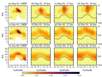
Figure 7.Temporal evolution of the zonal mean aerosol extinction coefficient (km−1) at 1020 nm. Monthly mean latitude–height distributions in September 1991 (first row), December 1991 (second row), and June 1992 (third row). Observation-based CMIP6 aerosol data set (first column), and simulations with emission of SO2at 16 km (second column), 17 km (third column), and 18 km (fourth column). The vertical
axis shows the height in km and the black line indicates the modelled tropopause.
The resulting spatial distribution of the aerosol extinction coefficient is compared to satellite and ground-based ob-servations that are compiled in the CMIP6 aerosol data set (L. Beiping, personal communication, 2016) in Fig. 7. The simulation with emission of SO2 at 17 km was selected as the best fit, because the height of the maximum extinction coefficient at 1020 nm in September and December 1991 is closest to the CMIP6 data. In contrast, emission at 16 km re-sults in faster meridional transport in the lower stratosphere and therefore an overly fast decrease in aerosol extinction af-ter the eruption, while emission at 18 km produces an aerosol layer considerably higher in altitude than observed.
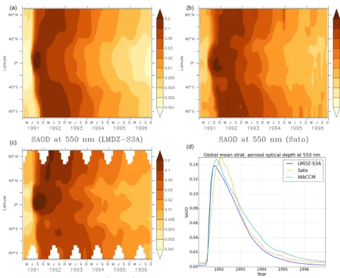
The modelled evolution of the SAOD at 550 nm is also compared to a climatology from Sato (2012) and to SAOD simulated with the WACCM model by Mills et al. (2016) in Fig. 8. The global mean SAOD increases a little faster in LMDZ-S3A than in the Sato climatology, but just as fast as in WACCM. LMDZ-S3A slightly underestimates the maxi-mum value of 0.15 from the Sato climatology and decreases at approximately the same rate of 7–8 % per month, while the decrease in WACCM, which includes several minor volcanic eruptions after Pinatubo, is slower. All three latitudinal distri-butions of the zonal mean SAOD are overall in good agree-ment, but with an earlier decrease in the tropics in LMDZ-S3A and with a stronger asymmetry towards the Northern Hemisphere in the WACCM simulation.
Figure 9 shows that the 7 Tg S emitted as SO2during the eruption are quickly converted into particles. The aerosol burden reaches its maximum 4 months after the eruption and then decreases slowly until it reaches a background value again after 4 to 5 years. The H2SO4burden increases more slowly than the aerosol, probably because it requires more time to transport the sulfur to the higher stratosphere. This is the only region where a larger reservoir of sulfuric acid vapour can remain because particles tend to evaporate at the local temperature and pressure.
Particle size is compared to the continuous optical parti-cle counter (OPC) measurements by Deshler et al. (2003) at 41◦N in Figs. 10 and 11.
Figure 8.Evolution of the zonal mean stratospheric aerosol optical depth (SAOD) at 550 nm modelled with LMDZ-S3A(a)compared to the climatology from Sato (2012)(b)and to SAOD simulated with WACCM by Mills et al. (2016)(c), as well as the global mean SAOD(d). Note that, unlike our simulation, WACCM includes small volcanic eruptions that occurred after that of Mount Pinatubo.
In Fig. 11 the modelled and observed particle size distribu-tions 5, 11, and 17 months after the eruption are compared. The model tends to overestimate particle concentrations of all size bins in the higher stratosphere, but reproduces the ob-servations ofr >0.01 andr >0.15 µm particles fairly well at lower levels. The concentration ofr >0.5 µm particles is underestimated at the height of highest concentrations (17– 21 km).
3.3 Sensitivity studies under Pinatubo conditions 3.3.1 Sensitivity to van der Waals coagulation
enhancement factor
In LMDZ-S3A we have only considered Brownian coag-ulation (Jacobson et al., 1994). Other terms for coagula-tion include those due to van der Waals forces,
per-1992 1993 1994 1995 1996 Year
0 1 2 3
Tg (S)
Figure 9.Evolution of the modelled stratospheric sulfur burden and its distribution among the different species for the period from Jan-uary 1991 to December 1996, including the Pinatubo eruption (but no other eruptions).
1991 1992 1993 1994 1995 1996 1997 Year
0.1 0.2 0.3 0.4 0.5 0.6 0.7 0.8
Effective
radius
(
µ
m)
Effective radius averaged for 14–30 km altitude at Laramie
LMDZ-S3A LMDZ-S3A (onlyrdry>0.15µm) Obs. (Deshler)
Figure 10. Stratospheric effective particle radius at Laramie, Wyoming (41◦N, 105◦W), as simulated by the LMDZ-S3A model and observed with optical particle counters (Deshler et al., 2003). Error bars of the measurements were determined from the 40 % uncertainty in aerosol surface area Aand volume V assuming a correlation coefficient of 0.5 betweenAat different altitudes,V at different altitudes, andAandV at the same altitude.
formed two additional simulations of the Pinatubo eruption: a first one with coagulation enhanced uniformly by the fac-torE(0)and a second one with coagulation enhanced uni-formly by the factor E(∞)(which is generally larger than
E(0)). For colliding particles of identical size and a tempera-ture of 298 K,E(0)andE(∞)have values of 1.25 and 2.27, respectively. The actual enhancement factor for stratospheric conditions can be expected to lie in between these two cases. As in previous studies, the van der Waals coagulation term improves the comparison to observation for particle number concentration (not shown) and particle average size (shown in Fig. 12), but it makes it a little worse for AOD, as shown in Fig. 13, with the global mean stratospheric AOD peaking too low (and too early) compared to the Sato climatology. Given
10−510−410−310−210−1 100 101 102 103
Number conc. [1/cm3]
14 16 18
Altitude OPC rOPC r>>0.010.15µµmm OPC r>0.50µm
10−510−410−310−210−1 100 101 102 103
Number conc. [1/cm3]
14 16 18 20 22 24 26 28 30
Altitude
[km]
(b) May 1992
10−510−410−310−210−1 100 101 102 103
Number conc. [1/cm3]
14 16 18 20 22 24 26 28 30
Altitude
[km]
(c) November 1992
Figure 11.Vertical profile of the cumulative aerosol number con-centration (cm−3) for three channels (r >0.01 µm in light blue,
r >0.15 µm in orange, and r >0.5 µm in dark blue) in Novem-ber 1991, May 1992, and NovemNovem-ber 1992 at Laramie, Wyoming (41◦N, 105◦W), in the style of Sekiya et al. (2016). Solid lines show the modelled monthly mean, while the crosses indicate the range of daily mean concentrations within that month. Optical par-ticle counter (OPC) measurements from Deshler et al. (2003) are shown as symbols.
that there are only a few measurements to constrain the van der Waals coagulation term, and the mixed results obtained in our model, we do not include this process in our default model, but offer it as an option in the code of the model. 3.3.2 Sensitivity to the SO2chemical lifetime
1991 1992 1993 1994 1995 1996 1997 Year
0.1 0.2 0.3 0.4 0.5 0.6 0.7 0.8
Effective
radius
(
µ
m)
Effective radius averaged for 14–30 km altitude at Laramie
LMDZ-S3A LMDZ-S3A (vdW factorE(0)) LMDZ-S3A (vdW factorE(∞)) Obs. (Deshler)
Figure 12. Stratospheric effective particle radius at Laramie, Wyoming (41◦N, 105◦W), as simulated by the LMDZ-S3A model and observed with optical particle counters (Deshler et al., 2003). The light blue (orange) line shows the model result for coagulation enhanced by the continuum regime van der Waals enhancement fac-torE(0)(the kinetic regime enhancement factorE(∞)).
the sensitivity of our results to the assumed global SO2 re-moval rate, we performed another Pinatubo simulation with SO2lifetimes increased by a factor of 2 on the day of the eruption and decreasing linearly to normal values within 1 month. It appears unlikely that the OH effect impacted the global SO2 lifetime beyond this factor of 2, notably when compared with observational studies of the volcanic SO2 de-cay. Analyses of SO2observations after the eruption give a global SO2lifetime ranging from 23 to 35 days (Bluth et al., 1992; Read et al., 1993). We find that the increase in assumed SO2 lifetime delays and increases slightly the peak of the global mean AOD (shown in Fig. 14). However, overall the sensitivity to the SO2 lifetime appears to be small. There-fore we conclude that using a prescribed chemical lifetime is probably not a major limitation of our model, except for very large SO2injection rates, although it is desirable of course to improve the model in that respect in future studies.
4 Conclusions
In this article we have presented a newly developed sec-tional stratospheric sulfate aerosol (S3A) model as part of the LMDZ atmospheric general circulation model. A strength of our model is that it can readily be coupled to other compo-nents of the IPSL climate (and Earth system) model to per-form climate studies. The S3A model includes a represen-tation of sulfate particles with dry radii between 1 nm and 3.3 µm in currently 36 size bins, as well as the precursor gases OCS, SO2, and H2SO4. The aerosol-relevant physical processes of nucleation, condensation, evaporation, coagula-tion, and sedimentation are represented together with inter-active aerosol optical properties and radiative transfer in 6
1991 1992 1993 1994 1995 1996 1997 Year
0.00 0.02 0.04 0.06 0.08 0.10 0.12 0.14 0.16 0.18
SAOD
Global mean strat. AOD at 550 nm
LMDZ-S3A LMDZ-S3A (vdW factorE(0)) LMDZ-S3A (vdW factorE(∞)) Sato
WACCM
Figure 13.Evolution of the global mean stratospheric aerosol opti-cal depth (SAOD) at 550 nm modelled with LMDZ-S3A compared to the climatology from Sato (2012) and to SAOD simulated with WACCM by Mills et al. (2016). The dashed (dotted) line shows the model result for coagulation enhanced by the continuum regime van der Waals enhancement factorE(0)(the kinetic regime enhance-ment factorE(∞)).
1991 1992 1993 1994 1995 1996 1997 Year
0.00 0.02 0.04 0.06 0.08 0.10 0.12 0.14 0.16 0.18
SAOD
Global mean strat. AOD at 550 nm
LMDZ-S3A LMDZ-S3A (τ(SO2) increased for 1 month) Sato WACCM
Figure 14.Same as Fig. 13, but here the dashed line shows the model result for an SO2lifetime doubled on the day of the eruption, decreasing linearly to climatological values within 1 month.
solar and 16 terrestrial spectral bands. The tropospheric fate of stratospheric sulfate aerosols is also simulated.
of future work as S3A can be coupled to the REPROBUS model which is also part of the IPSL Earth system model. In-teractive ozone is also expected to help the model simulate a smaller heating rate and temperature anomaly in the presence of volcanic aerosols. Further developments will also include a more comprehensive treatment of the coagulation kernel and the possible interactions with other aerosol types (organ-ics and meteoritic dust) in the stratosphere.
Finally it has to be stated that it has been a non-trivial task to gather observations of stratospheric aerosols for model evaluation. A fully validated, gridded stratospheric aerosol climatology in an easily usable format (like netCDF) with information on how gap filling is performed would tremen-dously facilitate the evaluation of model results. The strato-spheric aerosol data set produced for CMIP6 (L. Beiping, personal communication, 2016) is a significant step in the right direction. Knowledge of (average) tropopause height would be particularly useful, so that vertically integrated quantities like AOD can be compared between model and observations and potential biases coming from differences in tropopause height can be detected. A more systematic re-porting of observational uncertainties from both in situ and satellite data would be welcomed. This request extends to the provision of error covariances between measured quantities as these are needed to compute the error budget of combi-nations of observed quantities (as is the case for the aerosol effective radius).
Code availability. The code of S3A can be downloaded along with the LMDZ model from http://lmdz.lmd.jussieu.fr. S3A code is mostly contained within a separate directory (StratAer) of the model physics and is activated at compilation with a CPP key. A model configuration (LMDZORSTRATAER_v6) containing the S3A module is also available within the modipsl/libIGCM model environment of the IPSL Earth system model (http://forge.ipsl. jussieu.fr/igcmg_doc).
Author contributions. CK developed most of the new parts of the model, performed the simulations, visualised and analysed the data, and wrote most of the article. OB had the original idea of the new model, assisted extensively in the development, evaluation, and analysis, and contributed to many parts of the written article. SB contributed the basis of the model code for condensation, evapora-tion, and aerosol composievapora-tion, and wrote parts of the sections on these processes and on the history of aerosol modelling. FL devel-oped and tuned the model’s interactive QBO and wrote the section on this. UP contributed to the discussions leading to and accompa-nying the model development.
viding a compilation of stratospheric aerosol observation data and Josefine Ghattas for preparing the LMDZORSTRATAER_v6 configuration. The authors acknowledge computing time from the TGCC under GENCI projects t2014012201, t2015012201, t2016012201, and t2017012201. The authors would like to thank two anonymous reviewers for their constructive comments, and the editor, Graham Mann, for his editorial review of the first submitted version of this paper, which led to significant improvements to the introduction section.
Edited by: Graham Mann
Reviewed by: two anonymous referees
References
Aquila, V., Oman, L. D., Stolarski, R. S., Colarco, P. R., and New-man, P. A.: Dispersion of the volcanic sulfate cloud from a Mount Pinatubo-like eruption, J. Geophys. Res.-Atmos., 117, D06216, https://doi.org/10.1029/2011JD016968, 2012.
Ayers, G. P., Gillett, R. W., and Gras, J. L.: On the vapor pressure of sulfuric acid, Geophys. Res. Lett., 7, 433–436, https://doi.org/10.1029/GL007i006p00433, 1980.
Bekki, S.: Oxidation of volcanic SO2: A sink for
strato-spheric OH and H2O, Geophys. Res. Lett., 22, 913–916,
https://doi.org/10.1029/95GL00534, 1995.
Bekki, S. and Pyle, J. A.: Two-dimensional assessment of the impact of aircraft sulphur emissions on the stratospheric sul-phate aerosol layer, J. Geophys. Res.-Atmos., 97, 15839–15847, https://doi.org/10.1029/92JD00770, 1992.
Bekki, S. and Pyle, J. A.: Potential impact of combined NOx and
SOxemissions from future high speed civil transport aircraft on
stratospheric aerosols and ozone, Geophys. Res. Lett., 20, 723– 726, https://doi.org/10.1029/93GL00853, 1993.
Bluth, G. J. S., Doiron, S. D., Schnetzler, C. C., Krueger, A. J., and Walter, L. S.: Global tracking of the SO2clouds from the June, 1991 Mount Pinatubo eruptions, Geophys. Res. Lett., 19, 151– 154, https://doi.org/10.1029/91GL02792, 1992.
Budyko, M. I.: Climatic Changes, American Geophysical Union, https://doi.org/10.1029/SP010, 1977.
Chan, T. W. and Mozurkewich, M.: Measurement of the co-agulation rate constant for sulfuric acid particles as a func-tion of particle size using tandem differential mobility analy-sis, J. Aerosol Sci., 32, 321–339, https://doi.org/10.1016/S0021-8502(00)00081-1, 2001.
Crutzen, P. J.: Albedo Enhancement by Stratospheric Sulfur Injec-tions: A Contribution to Resolve a Policy Dilemma?, Climatic Change, 77, 211–219, https://doi.org/10.1007/s10584-006-9101-y, 2006.
Deshler, T.: A review of global stratospheric aerosol: Measurements, importance, life cycle, and local stratospheric aerosol, Atmos. Res., 90, 223–232, https://doi.org/10.1016/j.atmosres.2008.03.016, 2008.
Deshler, T., Hervig, M. E., Hofmann, D. J., Rosen, J. M., and Liley, J. B.: Thirty years of in situ stratospheric aerosol size distri-bution measurements from Laramie, Wyoming (41◦N), using balloon-borne instruments, J. Geophys. Res.-Atmos., 108, 4167, https://doi.org/10.1029/2002JD002514, 2003.
Dhomse, S. S., Emmerson, K. M., Mann, G. W., Bellouin, N., Carslaw, K. S., Chipperfield, M. P., Hommel, R., Abraham, N. L., Telford, P., Braesicke, P., Dalvi, M., Johnson, C. E., O’Connor, F., Morgenstern, O., Pyle, J. A., Deshler, T., Za-wodny, J. M., and Thomason, L. W.: Aerosol microphysics simulations of the Mt. Pinatubo eruption with the UM-UKCA composition-climate model, Atmos. Chem. Phys., 14, 11221– 11246, https://doi.org/10.5194/acp-14-11221-2014, 2014. Dufresne, J.-L., Foujols, M.-A., Denvil, S., Caubel, A., Marti, O.,
Aumont, O., Balkanski, Y., Bekki, S., Bellenger, H., Benshila, R., Bony, S., Bopp, L., Braconnot, P., Brockmann, P., Cadule, P., Cheruy, F., Codron, F., Cozic, A., Cugnet, D., de Noblet, N., Duvel, J.-P., Ethé, C., Fairhead, L., Fichefet, T., Flavoni, S., Friedlingstein, P., Grandpeix, J.-Y., Guez, L., Guilyardi, E., Hauglustaine, D., Hourdin, F., Idelkadi, A., Ghattas, J., Jous-saume, S., Kageyama, M., Krinner, G., Labetoulle, S., Lahel-lec, A., Lefebvre, M.-P., Lefevre, F., Levy, C., Li, Z. X., Lloyd, J., Lott, F., Madec, G., Mancip, M., Marchand, M., Masson, S., Meurdesoif, Y., Mignot, J., Musat, I., Parouty, S., Polcher, J., Rio, C., Schulz, M., Swingedouw, D., Szopa, S., Talandier, C., Terray, P., Viovy, N., and Vuichard, N.: Climate change projections us-ing the IPSL-CM5 Earth System Model: from CMIP3 to CMIP5, Clim. Dynam., 40, 2123–2165, https://doi.org/10.1007/s00382-012-1636-1, 2013.
Dutton, E. G. and Christy, J. R.: Solar radiative forcing at selected locations and evidence for global lower tropospheric cooling fol-lowing the eruptions of El Chichón and Pinatubo, Geophys. Res. Lett., 19, 2313–2316, https://doi.org/10.1029/92GL02495, 1992. English, J. M., Toon, O. B., Mills, M. J., and Yu, F.: Microphysical simulations of new particle formation in the upper troposphere and lower stratosphere, Atmos. Chem. Phys., 11, 9303–9322, https://doi.org/10.5194/acp-11-9303-2011, 2011.
English, J. M., Toon, O. B., and Mills, M. J.: Microphys-ical simulations of large volcanic eruptions: Pinatubo and Toba, J. Geophys. Res.-Atmos., 118, 1880–1895, https://doi.org/10.1002/jgrd.50196, 2013.
Escribano, J., Boucher, O., Chevallier, F., and Huneeus, N.: Subregional inversion of North African dust sources, J. Geophys. Res.-Atmos., 121, 8549–8566, https://doi.org/10.1002/2016JD025020, 2016.
Eyring, V., Bony, S., Meehl, G. A., Senior, C. A., Stevens, B., Stouffer, R. J., and Taylor, K. E.: Overview of the Coupled Model Intercomparison Project Phase 6 (CMIP6) experimen-tal design and organization, Geosci. Model Dev., 9, 1937–1958, https://doi.org/10.5194/gmd-9-1937-2016, 2016.
Flato, G., Marotzke, J., Abiodun, B., Braconnot, P., Chou, S., Collins, W., Cox, P., Driouech, F., Emori, S., Eyring, V., For-est, C., Gleckler, P., Guilyardi, E., Jakob, C., Kattsov, V., Rea-son, C., and Rummukainen, M.: Evaluation of Climate Mod-els, in: Climate Change 2013: The Physical Science Basis.
Contribution of Working Group I to the Fifth Assessment Report of the Intergovernmental Panel on Climate Change, edited by: Stocker, T., Qin, D., Plattner, G.-K., Tignor, M., Allen, S., Boschung, J., Nauels, A., Xia, Y., Bex, V., and Midgley, P., book section 9, 741–866, Cambridge University Press, Cambridge, United Kingdom and New York, NY, USA, https://doi.org/10.1017/CBO9781107415324.020, 2013. Fouquart, Y. and Bonnel, B.: Computations of solar heating of
the earth’s atmosphere – A new parameterization, Beitraege zur Physik der Atmosphaere, 53, 35–62, 1980.
Garcia, R. R., Marsh, D. R., Kinnison, D. E., Boville, B. A., and Sassi, F.: Simulation of secular trends in the middle at-mosphere, 1950–2003, J. Geophys. Res.-Atmos., 112, D09301, https://doi.org/10.1029/2006JD007485, 2007.
Giauque, W., Hornung, E., Kunzler, J., and Rubin, T.: The ther-modynamic properties of aqueous sulfuric acid solutions and hydrates from 15 to 300 K, J. Am. Chem. Soc., 82, 62–70, https://doi.org/10.1021/ja01486a014, 1960.
Giorgetta, M. A., Manzini, E., Roeckner, E., Esch, M., and Bengts-son, L.: Climatology and Forcing of the Quasi-Biennial Oscil-lation in the MAECHAM5 Model, J. Climate, 19, 3882–3901, https://doi.org/10.1175/JCLI3830.1, 2006.
Gmitro, J. I. and Vermeulen, T.: Vapor-liquid equilib-ria for aqueous sulfuric acid, AICHE J., 10, 740–746, https://doi.org/10.1002/aic.690100531, 1964.
Hamill, P., Turco, R., Kiang, C., Toon, O., and Whitten, R.: An analysis of various nucleation mechanisms for sulfate particles in the stratosphere, J. Aerosol Sci., 13, 561–585, https://doi.org/10.1016/0021-8502(82)90021-0, 1982.
Haywood, J. M., Jones, A., Clarisse, L., Bourassa, A., Barnes, J., Telford, P., Bellouin, N., Boucher, O., Agnew, P., Clerbaux, C., Coheur, P., Degenstein, D., and Braesicke, P.: Observations of the eruption of the Sarychev volcano and simulations using the HadGEM2 climate model, J. Geophys. Res.-Atmos., 115, D21212, https://doi.org/10.1029/2010JD014447, 2010. Hourdin, F. and Armengaud, A.: The Use of Finite-Volume
Methods for Atmospheric Advection of Trace Species. Part I: Test of Various Formulations in a General Circulation Model, Mon. Weather Rev., 127, 822–837, https://doi.org/10.1175/1520-0493(1999)127<0822:TUOFVM>2.0.CO;2, 1999.
Hourdin, F., Musat, I., Bony, S., Braconnot, P., Codron, F., Dufresne, J.-L., Fairhead, L., Filiberti, M.-A., Friedlingstein, P., Grandpeix, J.-Y., Krinner, G., LeVan, P., Li, Z.-X., and Lott, F.: The LMDZ4 general circulation model: climate per-formance and sensitivity to parametrized physics with em-phasis on tropical convection, Clim. Dynam., 27, 787–813, https://doi.org/10.1007/s00382-006-0158-0, 2006.
Hourdin, F., Foujols, M.-A., Codron, F., Guemas, V., Dufresne, J.-L., Bony, S., Denvil, S., Guez, J.-L., Lott, F., Ghattas, J., Braconnot, P., Marti, O., Meurdesoif, Y., and Bopp, L.: Impact of the LMDZ atmospheric grid configuration on the climate and sensitivity of the IPSL-CM5A coupled model, Clim. Dynam., 40, 2167–2192, https://doi.org/10.1007/s00382-012-1411-3, 2013.
Jacobson, M. Z., Turco, R. P., Jensen, E. J., and Toon, O. B.: Modeling coagulation among particles of differ-ent composition and size, Atmos. Environ., 28, 1327–1338, https://doi.org/10.1016/1352-2310(94)90280-1, 1994.
Kawatani, Y. and Hamilton, K.: Weakened stratospheric quasibien-nial oscillation driven by increased tropical mean upwelling, Na-ture, 497, 478–481, https://doi.org/10.1038/nature12140, 2013. Kokkola, H., Hommel, R., Kazil, J., Niemeier, U., Partanen, A.-I.,
Feichter, J., and Timmreck, C.: Aerosol microphysics modules in the framework of the ECHAM5 climate model – intercomparison under stratospheric conditions, Geosci. Model Dev., 2, 97–112, https://doi.org/10.5194/gmd-2-97-2009, 2009.
Kovilakam, M. and Deshler, T.: On the accuracy of stratospheric aerosol extinction derived from in situ size distribution measure-ments and surface area density derived from remote SAGE II and HALOE extinction measurements, J. Geophys. Res.-Atmos., 120, 8426–8447, https://doi.org/10.1002/2015JD023303, 2015. Kremser, S., Thomason, L. W., von Hobe, M., Hermann, M.,
Desh-ler, T., Timmreck, C., Toohey, M., Stenke, A., Schwarz, J. P., Weigel, R., Fueglistaler, S., Prata, F. J., Vernier, J.-P., Schlager, H., Barnes, J. E., Antuña-Marrero, J.-C., Fairlie, D., Palm, M., Mahieu, E., Notholt, J., Rex, M., Bingen, C., Vanhellemont, F., Bourassa, A., Plane, J. M. C., Klocke, D., Carn, S. A., Clarisse, L., Trickl, T., Neely, R., James, A. D., Rieger, L., Wil-son, J. C., and Meland, B.: Stratospheric aerosol – Observations, processes, and impact on climate, Rev. Geophys., 54, 278–335, https://doi.org/10.1002/2015RG000511, 2016.
Krinner, G., Viovy, N., de Noblet-Ducoudré, N., Ogée, J., Polcher, J., Friedlingstein, P., Ciais, P., Sitch, S., and Prentice, I. C.: A dynamic global vegetation model for studies of the cou-pled atmosphere-biosphere system, Global Biogeochem. Cy., 19, GB1015, https://doi.org/10.1029/2003GB002199, 2005. Lefèvre, F., Brasseur, G. P., Folkins, I., Smith, A. K., and Simon,
P.: Chemistry of the 1991–1992 stratospheric winter: Three-dimensional model simulations, J. Geophys. Res.-Atmos., 99, 8183–8195, https://doi.org/10.1029/93JD03476, 1994.
Lefèvre, F., Figarol, F., Carslaw, K. S., and Peter, T.: The 1997 Arctic Ozone depletion quantified from three-dimensional model simulations, Geophys. Res. Lett., 25, 2425–2428, https://doi.org/10.1029/98GL51812, 1998.
Lott, F. and Guez, L.: A stochastic parameterization of the grav-ity waves due to convection and its impact on the equato-rial stratosphere, J. Geophys. Res.-Atmos., 118, 8897–8909, https://doi.org/10.1002/jgrd.50705, 2013.
Lott, F., Denvil, S., Butchart, N., Cagnazzo, C., Giorgetta, M. A., Hardiman, S. C., Manzini, E., Krismer, T., Duvel, J.-P., Maury, P., Scinocca, J. F., Watanabe, S., and Yukimoto, S.: Kelvin and Rossby-gravity wave packets in the lower stratosphere of some high-top CMIP5 models, J. Geophys. Res.-Atmos., 119, 2156– 2173, https://doi.org/10.1002/2013JD020797, 2014.
MacMartin, D. G., Kravitz, B., Long, J. C. S., and Rasch, P. J.: Geoengineering with stratospheric aerosols: What do we not
Manktelow, P. T., Chipperfield, M. P., Pickering, S. J., and Johnson, C. E.: Description and evaluation of GLOMAP-mode: a modal global aerosol microphysics model for the UKCA composition-climate model, Geosci. Model Dev., 3, 519–551, https://doi.org/10.5194/gmd-3-519-2010, 2010.
Mills, M. J., Toon, O. B., and Solomon, S.: A 2D microphysical model of the polar stratospheric CN layer, Geophys. Res. Lett., 26, 1133–1136, https://doi.org/10.1029/1999GL900187, 1999. Mills, M. J., Schmidt, A., Easter, R., Solomon, S.,
Kinni-son, D. E., Ghan, S. J., Neely, R. R., Marsh, D. R., Con-ley, A., Bardeen, C. G., and Gettelman, A.: Global volcanic aerosol properties derived from emissions, 1990–2014, using CESM1(WACCM), J. Geophys. Res.-Atmos., 121, 2332–2348, https://doi.org/10.1002/2015JD024290, 2016.
Mlawer, E. J., Taubman, S. J., Brown, P. D., Iacono, M. J., and Clough, S. A.: Radiative transfer for inhomogeneous atmospheres: RRTM, a validated correlated-k model for the longwave, J. Geophys. Res.-Atmos., 102, 16663–16682, https://doi.org/10.1029/97JD00237, 1997.
Oman, L., Robock, A., Stenchikov, G. L., Thordarson, T., Koch, D., Shindell, D. T., and Gao, C.: Modeling the dis-tribution of the volcanic aerosol cloud from the 1783– 1784 Laki eruption, J. Geophys. Res.-Atmos., 111, D12209, https://doi.org/10.1029/2005JD006899, 2006.
Pinto, J. P., Turco, R. P., and Toon, O. B.: Self-limiting physical and chemical effects in volcanic eruption clouds, J. Geophys. Res.-Atmos., 94, 11165–11174, https://doi.org/10.1029/JD094iD08p11165, 1989.
Pitari, G., Mancini, E., Rizi, V., and Shindell, D. T.: Impact of Future Climate and Emission Changes on Stratospheric Aerosols and Ozone, J. Atmos. Sci., 59, 414–440, https://doi.org/10.1175/1520-0469(2002)059<0414:IOFCAE>2.0.CO;2, 2002.
Pruppacher, H. R. and Klett, J. D.: Microphysics of Clouds and Precipitation, Springer Science & Business Media, https://doi.org/10.1007/978-0-306-48100-0, 2010.
Read, W. G., Froidevaux, L., and Waters, J. W.: Microwave limb sounder measurement of stratospheric SO2 from the Mt. Pinatubo Volcano, Geophys. Res. Lett., 20, 1299–1302, https://doi.org/10.1029/93GL00831, 1993.
Reichler, T., Dameris, M., and Sausen, R.: Determining the tropopause height from gridded data, Geophys. Res. Lett., 30, 2042, https://doi.org/10.1029/2003GL018240, 2003.
Ridley, D. A., Solomon, S., Barnes, J. E., Burlakov, V. D., Desh-ler, T., Dolgii, S. I., Herber, A. B., Nagai, T., Neely, R. R., Nevzorov, A. V., Ritter, C., Sakai, T., Santer, B. D., Sato, M., Schmidt, A., Uchino, O., and Vernier, J. P.: Total vol-canic stratospheric aerosol optical depths and implications for global climate change, Geophys. Res. Lett., 41, 7763–7769, https://doi.org/10.1002/2014GL061541, 2014.