Geosci. Model Dev., 7, 3017–3035, 2014 www.geosci-model-dev.net/7/3017/2014/ doi:10.5194/gmd-7-3017-2014
© Author(s) 2014. CC Attribution 3.0 License.
A global finite-element shallow-water model supporting continuous
and discontinuous elements
P. A. Ullrich1,2
1Department of Land, Air and Water Resources, University of California, Davis, One Shields Ave., Davis, CA 95616, USA 2Lawrence Berkeley National Laboratory, Berkeley, CA 94720, USA
Correspondence to: P. A. Ullrich ([email protected])
Received: 8 July 2014 – Published in Geosci. Model Dev. Discuss.: 8 August 2014 Revised: 31 October 2014 – Accepted: 5 November 2014 – Published: 17 December 2014
Abstract. This paper presents a novel nodal finite-element method for either continuous and discontinuous elements, as applied to the 2-D shallow-water equations on the cubed sphere. The cornerstone of this method is the construction of a robust derivative operator that can be applied to compute discrete derivatives even over a discontinuous function space. A key advantage of the robust derivative is that it can be ap-plied to partial differential equations in either a conservative or a non-conservative form. However, it is also shown that discontinuous penalization is required to recover the correct order of accuracy for discontinuous elements. Two versions with discontinuous elements are examined, using either the
g1andg2flux correction function for distribution of bound-ary fluxes and penalty across nodal points. Scalar and vector hyperviscosity (HV) operators valid for both continuous and discontinuous elements are also derived for stabilization and removal of grid-scale noise. This method is validated using four standard shallow-water test cases, including geostrophi-cally balanced flow, a mountain-induced Rossby wave train, the Rossby–Haurwitz wave and a barotropic instability. The results show that although the discontinuous basis requires a smaller time step size than that required for continuous elements, the method exhibits better stability and accuracy properties in the absence of hyperviscosity.
1 Introduction
Modeling of the 2-D shallow-water equations is an impor-tant step in understanding the behavior of a numerical dis-cretization for atmospheric modeling. In particular, the dy-namical character of the global shallow-water equations is
governed by features common with atmospheric motions in-cluding nonlinearity, barotropic Rossby waves and inertia-gravity waves, without the added complexity of a vertical di-mension.
A comprehensive literature already exists on the devel-opment of numerical methods for the global shallow-water equations spanning the past several decades. Examples in-clude the spectral transform method (Jakob-Chien et al., 1995), semi-Lagrangian methods (Ritchie, 1988; Bates et al., 1990; Tolstykh, 2002; Zerroukat et al., 2009; Tolstykh and Shashkin, 2012; Qaddouri et al., 2012), finite-difference methods (Heikes and Randall, 1995; Ronchi et al., 1996), Godunov-type finite-volume methods (Rossmanith, 2006; Ullrich et al., 2010), staggered finite-volume methods (Lin and Rood, 1997; Ringler et al., 2008, 2011), multi-moment finite-volume methods (Chen and Xiao, 2008; Li et al., 2008; Chen et al., 2014) and finite-element methods (Taylor et al., 1997; Côté and Staniforth, 1990; Thomas and Loft, 2005; Giraldo et al., 2002; Nair et al., 2005; Läuter et al., 2008; Comblen et al., 2009; Bao et al., 2014).
oper-3018 P. A. Ullrich: A global finite-element shallow-water model ator which is valid for continuous or discontinuous elements
and only requires one communication per application of the Laplacian.
Discontinuous elements are potentially more desirable than continuous elements for several reasons: first, discon-tinuous elements only require parallel communication along coordinate axes, whereas continuous elements also require parallel communication along diagonals, a doubling of the total number of communications in 2-D. Second, discontin-uous elements provide a natural mechanism to enforce stabi-lization via discontinuous penastabi-lization (or Riemann solvers, for equations in conservation form). Third, discontinuous el-ements can be used in conjunction with upwind methods, which are generally better for tracer transport and associ-ated problems. However, discontinuous elements also have a number of disadvantages, including higher storage require-ments (for the same order of accuracy), a maximum time step size which is typically smaller than that imposed for contin-uous elements (Ullrich, 2013) and added computational ex-pense for many hyperbolic operations.
The outline of this paper is as follows. Section 2 presents the shallow-water equations on a manifold. The cubed-sphere grid, which will be used for simulations on the cubed-sphere, is described in Sect. 3. The discretizations of the dynamics and hyperviscosity (HV) are then presented in Sects. 4 and 5, respectively. Results from four standard shallow-water test cases are given in Sect. 6 and conclusions follow in Sect. 7.
2 The shallow-water equations on a manifold
The 2-D shallow-water equations in on a Riemannian mani-fold with coordinate indicesxs= {α, β}can be written as
∂uα ∂t +u
s∇
suα+gαs
∂
∂xs(gcH )+f (k×u)
α=0, (1)
∂uβ ∂t +u
s∇
suβ+gβs
∂
∂xs(gcH )+f (k×u)
β =0, (2)
∂H
∂t + ∇s(hu
s)=0. (3) The prognostic variables are free-surface height H and vector velocity u=uαgα+uβgβ, wheregα=∂x/∂αand gβ=∂x/∂β are the natural basis vectors on the manifold. The fluid height h and height of the bottom topography z
are related to the free-surface height via H=h+z. Here
grs denotes the contravariant metric with covariant inverse
grs,J= √
detgrs is the metric Jacobian,gc is gravity,f is the Coriolis parameter andk is the vertical basis vector of unit length. The Einstein summation notation (implied sum-mation) is used for repeated indices. These equations further make use of the covariant derivative∇s, which expands as
us∇sud=uα∂u
d
∂α +u
β∂ud
∂β +0
d
srusur, (4)
∇s(hus)= 1
J ∂ ∂α(J hu
α)+1
J ∂ ∂β(J hu
β), (5)
Discussion
P
ap
er
|
Dis
cussion
P
ap
er
|
Discussion
P
ap
er
|
Discussion
P
ap
er
|
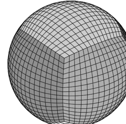
Fig. 1.A 3D view of the cubed-sphere grid shown here withne= 16. Cubed sphere faces are individually
shaded.
36
Figure 1. A 3-D view of the cubed-sphere grid shown here with
ne=16. Cubed-sphere faces are individually shaded.
where0dsrdenote the Christoffel symbols of the second kind associated with the coordinate transform (again with summa-tion over repeated indicessandrimplied).
The mass equation, Eq. (3), has been kept in conservative form to enforce strict mass conservation. On the other hand, Eqs. (1)–(2) are given in a non-conservative form; this for-mulation is selected over the flux-form equations (wherehuα
andhuβ are prognostic variables). Angular momentum and potential enstrophy are particularly relevant to atmospheric motions (Thuburn, 2008) and can be easily conserved under a non-conservative formulation of the shallow-water equations (Taylor and Fournier, 2010). Conservation of these quantities is more difficult when they are diagnosed from the flux-form prognostic variables. The non-conservative formulation also has the advantage of leading to a more accurate treatment of wave-like motion when formulated appropriately (Thuburn and Woollings, 2005).
3 The cubed-sphere grid
The Eqs. (1)–(3) are now applied to a particular choice of coordinate system. The cubed-sphere grid (Sadourny, 1972; Ronchi et al., 1996) consists of a cube with six Cartesian patches arranged along each face, which is then inflated onto a tangent spherical shell, as shown in Fig. 1. The cubed sphere is a quasi-uniform spherical grid, that is, it is in the class of grids that provide an approximately uniform tiling of the sphere (see Staniforth and Thuburn (2012), for exam-ple, for a review of different options for global grids). On the equiangular cubed-sphere grid, coordinates are given as
(α, β, p), with central anglesα, β∈ [−π 4,
π
4]and panel index
P. A. Ullrich: A global finite-element shallow-water model 3019 be along the equator and panels 5 and 6 to be centered on
the northern and southern pole, respectively. With uniform grid spacing, each panel consists of a square array ofne×ne elements.
The contravariant 2-D metric on the equiangular cubed sphere of radiusais given by
grs= δ
2
a2(1+tan2α)(1+tan2β)
1+tan2β tanαtanβ
tanαtanβ 1+tan2α
, (6)
whereδ=p1+tan2α+tan2β. The Jacobian on the mani-fold, denoted byJ, is then
J =pdet(grs)=
a2(1+tan2α)(1+tan2β)
δ3 , (7)
and induces the infinitesimal area element dA=Jdαdβ. The Christoffel symbols of the second kind are given by
0αij=
2 tanαtan2β δ2
−tanβ (1+tan2β) δ2
−tanβ (1+tan2β)
δ2 0
, (8)
0βij=
0 −tanα (1+tan 2α)
δ2 −tanα (1+tan2α)
δ2
2tan2αtanβ δ2
. (9)
Spherical coordinates(λ, φ)for longitudeλ∈ [0,2π]and latitudeφ∈ [−π/2, π/2]will also be used for plotting and specification of tests. Coordinate transforms between spheri-cal and equiangular coordinates can be found in Ullrich and Jablonowski (2012) Appendix A.
4 Nodal finite-element discretization 4.1 The nodal basis
A nodal finite-element method is employed (Taylor et al., 1997; Giraldo et al., 2002; Hesthaven and Warburton, 2007). The 1-D reference element is defined as the interval x∈ [−1,1]along with a set of test functions φˆ(i)(x). The test functions are defined such that test function φˆ(i)(x) is the unique polynomial of degreenpthat is one at theith Gauss– Lobatto–Legendre (GLL) node ,i∈(0, . . ., np−1), and zero at all other GLL nodes. Each basis polynomial then has a corresponding weight, defined by
wi = 1 Z
−1 ˆ
φ(i)(x)dx. (10)
Discussion
P
ap
er
|
Dis
cussion
P
ap
er
|
Discussion
P
ap
er
|
Discussion
P
ap
er
|
↵
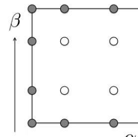
Fig. 2.A depiction of the nodal grid for a reference element on GLL nodes fornp= 4. Boundary nodes,
which are connected to neighboring elements, are shaded.
37
Figure 2. A depiction of the nodal grid for a reference element on
GLL nodes fornp=4. Boundary nodes, which are connected to
neighboring elements, are shaded.
The 2-D elementZ= [α1, α2] × [β1, β2](with boundary
∂Z) has accompanying 1-D basis functions
e
φ(i)(α)= ˆφ(i)
2(α−α 1)
1α −1
,
e
φ(j )(β)= ˆφ(j )
2(β−β 1)
1β −1
, (11)
where1α=α2−α1and1β=β2−β1. The accompanying 2-D tensor-product basis is then defined by
φ(i,j )(α, β)=eφ(i)(α)eφ(j )(β). (12)
Figure 2 provides a depiction of GLL nodes within a sin-gle element. For vector quantities (such as velocityu), test functions are instead vector fields. Uniqueness of the varia-tional system is retained if exactly 2 degrees of freedom are allowed at each nodal location for the vector test function φ. As we shall see, the most natural choice is test functions φ(α)(i,j )andφ(β)(i,j )with covariant components
φ(α)(i,j )α=φ(i,j ),φ(α)(i,j )β=0,φ (β)
(i,j )α=0,φ (β)
(i,j )β=φ(i,j ). (13)
4.2 Robust differentiation
A robust differentiation operator is now constructed for both continuous and discontinuous finite elements. Letf :
(α, β)→Rbe defined and continuous onZ∪∂Zwith basis
φ(i,j ):
f (α, β)= np−1
X
p=0 np−1
X
q=0
f(p,q)φ(p,q)(α, β), (14)
3020 P. A. Ullrich: A global finite-element shallow-water model
f (α, β) on∂Z, whereas no such restriction is imposed for discontinuous finite elements. Following Huynh (2007), ro-bust differentiation in theαdirection is defined at GLL nodes via
Dαf (αi, βj)= np−1
X
p=0
f(p,j )
∂eφ(p)
∂α (αi)
+dgR
dα (αi)(f(np−1,j )−f(np−1,j )) +dgL
dα(αi)(f(0,j )−f(0,j )), (15)
where the overscore denotes the co-located average off and e
f,
f(np−1,j )=
f (αnp−1, βj)+f (αe np−1, βj)
2 ,
f(0,j )=f (α0, βj)+f (αe 0, βj)
2 . (16)
An analogous definition holds in theβ direction. HeregL andgRare the local flux correction functions, which are cho-sen to satisfy
gL(α0)=1, gL(αnp−1)=0,
gR(α0)=0, gR(αnp−1)=1, (17)
and otherwise are chosen to approximate zero throughout [α0, αnp−1]. Several options forgLandgRwill lead to a
sta-ble discretization, includingg1(Radau polynomials), which will lead to the discontinuous Galerkin method, and g2, which will lead to the mass-lumped discontinuous Galerkin method (Huynh, 2007). Hereafter discontinuous elements with theg1flux correction function will be referred to as dis-continuous g1 elements, whereas elements using of the g2 flux correction function will be referred to as discontinuous
g2elements. Observe that for continuous finite elements, the rightmost two terms in Eq. (15) are exactly zero.
With the definition of a robust discrete derivative Eq. (15), discretization of the shallow-water system, Eqs. (1)–(3), is straightforward. Note that for continuous finite elements, this discretization is identical to the approach of Taylor et al. (1997) when applied in conjunction with direct stiffness sum-mation (DSS, that is, projection into the space of continu-ous functions; see Appendix A). If the conservative form of the shallow-water equations was employed, this discretiza-tion would be the same as Giraldo et al. (2002) when mass lumping is not employed (discontinuousg1) and Nair et al. (2005) if mass lumping is applied (discontinuousg2). To the best of the author’s knowledge, no previous work has used both discontinuous elements and a non-conservative form of the shallow-water system.
4.3 Discontinuous penalization
At element boundaries, the use of one-sided derivatives will cause the discontinuity between neighboring elements to
ex-hibit an error with magnitudeO(1xnp−1), an effective loss
of 1 order of accuracy from the expected convergence rate. To reduce errors associated with the discontinuity, a penal-ization term is added in each coordinate direction. In theα
direction this term reads as
∂H
∂t (αi, βj)=
. . .+∂gR ∂α(αi)
|λ(αnp−1, βj)|
2
e
H (αnp−1, βj)−H (αnp−1, βj)
J (αnp−1, βj)
J (αi, βj)
+∂gL ∂α (αi)
|λ(α0, βj)| 2
H (α0, βj)−H (αe 0, βj)
J (α0, βj)
J (αi, βj), (18)
∂ud
∂t (αi, βj)=
. . .+∂gR ∂α (αi)
|λ(αnp−1, βj)|
2
h eu
d(α
np−1, βj)−ud(αnp−1, βj)
i
+∂gL ∂α (αi)
|λ(α0, βj)| 2
h
ud(α0, βj)−
eu
d(α
0, βj)
i
, (19)
whereλ(α, β)= |uα| +√gh/arepresents the maximum lo-cal wave speed in theαdirection. An analogous term is added in theβ direction. Note that with this choice of penaliza-tion, the evolution equation forHis identical to the evolution equation that would arise from a traditional conservative dis-continuous Galerkin method with local Lax–Friedrichs flux. Since the penalization term is equivalent to upwinding, it is weakly diffusive and so allows the discontinuous scheme to maintain stability even in the absence of explicit viscosity.
4.4 Implementation considerations
On the cubed-sphere grid, the discontinuous method has 6n2en2p degrees of freedom compared to 8+8(ne(np−1)− 1)+6(ne(np−1)−1)2for the continuous method. In the limit asne→ ∞, this yields a ratio of(np−1)2/n2pdegrees of free-dom for the continuous formulation versus the discontinuous formulation. Note that in practice, the continuous formula-tion typically stores redundant degrees of freedom in order to reduce computational expense associated with indexing and so memory requirements are typically identical.
P. A. Ullrich: A global finite-element shallow-water model 3021 5 Viscosity and hyperviscosity
Stabilization is typically needed for co-located (or unstag-gered) finite-element methods, whether implicitly in the form of upwinding or explicitly in the form of a diffusive opera-tor, to avoid high-frequency dispersive errors associated with spectral ringing. In general, it is preferred that this operator is consistent with the underlying geometry of the Riemannian manifold, which precludes, for example, the Boyd–Vandeven filter (Boyd, 1996). There has been considerable success with the use of hyperviscosity in the spectral element method (Dennis et al., 2011), which maintains geometric consistency by mimicking the natural fourth-order hyperviscosity opera-tor. Previously, it has not been clear how to extend this oper-ator to a discontinuous function space. However, the robust derivative, Eq. (15), provides a direct mechanism by which the hyperviscosity operator can be constructed. The viscosity operator for both the continuous and discontinuous function space will be discussed here.
Note that any viscosity operator will lead to a loss of en-ergy conservation of the underlying numerical method. This loss is exhibited in two obvious ways: first, for geostrophi-cally balanced flows the error will tend to grow over time. Second, energy conservation is lost leading to a decay in the total energy content of the system over time.
5.1 Scalar viscosity
For stabilization of the method, diffusion is added in the form of either viscosity or hyperviscosity, which corresponds to multiple applications of the viscosity operator. A scalar vis-cosity operator is constructed to satisfy
H(ν)ψ≈ν∇2ψ, (20)
where ∇2= ∇ · ∇ is the usual scalar Laplacian. The oper-ator is defined implicitly via a variational construction. If
f =H(ν)ψthen, multiplying Eq. (20) by a test function and applying integration by parts, one obtains
Z Z
f φ(i,j )dA=
ν
I
∂Z
φ(i,j )∇ψ·dS− Z Z
Z
∇φ(i,j )· ∇ψdA
, (21)
where dSis the infinitesimal line element along the bound-ary of Z and dAis the infinitesimal area element. The two terms on the right-hand side of this expression correspond to the viscosity flux through element boundaries and the Lapla-cian within the element. Under a continuous element formu-lation, only the rightmost term is retained and fluxes are in-stead accounted for via direct stiffness summation. Under a discontinuous formulation, both terms are retained and dis-cretized. The discrete equation satisfied byf(i,j )that follows from Eq. (21) is written as
f(i,j )=f(i,j )B +f A
(i,j ), (22)
wheref(i,j )B denotes the discretization of the boundary inte-gral andf(i,j )A denotes the discretization of the area integral. After a lengthy derivation (see Appendix B), these discretiza-tions read as
f(i,j )A = − ν
wiJ (αi, βj) np−1
X
m=0 ∂eφ(i)
∂α ∇
α
ψ J wm
α=αm,β=βj
− ν
wjJ (αi, βj) np−1
X
n=0
∂eφ(j )
∂β ∇
β
ψ J wn
α=αi,β=βn, (23) and
f(i,j )B =
ν
δi,np−1
wi1α
∇αψ
| {z }
Right
+δj,np−1
wj1β
∇βψ
| {z }
Top
− δi,0
wi1α
∇αψ
| {z }
Left
− δj,0
wj1β
∇βψ
| {z }
Bottom
,
(24) where δi,j is the Krönecker delta. Here the contravariant derivative ofψhas been used, defined via
∇pψ=gpq∇qψ=gpα∂ψ ∂α +g
pβ∂ψ
∂β. (25)
Note that the contravariant derivatives ∇pψ are multi-valued along this edge, and so must be adjusted using the robust derivative operator Eq. (15).
5.2 Vector viscosity
Vector viscosity is used for damping of the velocity field, and takes the form
H(νd, νv)u≈νd∇(∇ ·u)−νv∇ ×(∇ ×u). (26) Observe that ifν=νd=νvthen this expression is exactly the standard vector Laplacian operator∇2u, with coefficient
ν. By writing the vector Laplacian as Eq. (26), the combined operator separates into two distinct operators that affect di-vergence damping (with coefficientνd) and vorticity damp-ing (with coefficientνv). This result can be quickly verified by taking the divergence and curl of Eq. (26),
∇ ·H(νd, νv)u=νd∇2(∇ ·u), (27) ∇ ×H(νd, νv)u= −νv∇ ×(∇ ×(∇ ×u))
=νv∇2(∇ ×u). (28)
For simplicity of calculation, we treat divergence damping and vorticity damping separately. For divergence damping, the operator is constructed by taking the inner product off= H(νd, νv)uwith the vector test functionφ, integrating over
Zand applying integration by parts,
νd Z Z
Z
φ·fdA=νd Z Z
Z
3022 P. A. Ullrich: A global finite-element shallow-water model
=νd
I
∂Z
(∇ ·u)φ·dS− Z Z
Z
(∇ ·φ)(∇ ·u)dV
. (29)
For vorticity damping an analogous procedure leads to
νv Z Z
Z
φ·fdA= −νv Z Z
Z
φ· ∇ ×(∇ ×u)dV ,
= −νv
I
∂Z
(∇ ×u)×φ·dS+ Z Z
Z
(∇ ×φ)·(∇ ×u)dV
.
(30) Note that for shallow-water flows, only the radial compo-nent of the vorticity is relevant for this calculation. The dis-crete value off(i,j )α andf(i,j )β that arises from this calculation then has contributions from the area integral via f(i,j )A,d and boundary integral viaf(i,j )B,d,
f(i,j )α =f(i,j )B,α+f(i,j )A,α, f(i,j )β =f(i,j )B,β+f(i,j )A,β. (31) Following another lengthy derivation (see Appendix B), the area integral term appears as
f(i,j )A,α=
− νd
J (αi, βj)wi np−1
X
m=0
J gααdeφ(i)
dα (∇ ·u)wm
α=αm,β=βj
− νd
J (αi, βj)wj np−1
X
n=0
J gβαdeφ(j )
dβ (∇ ·u)wn
α=α
i,β=βn
+ νv
J (αi, βj)wj np−1
X
n=0 deφ(j )
dβ (∇ ×u)rwn
α=αi,β=βn
, (32)
and
f(i,j )A,β=
− νd
J (αi, βj)wi np−1
X
m=0
J gαβdeφ(i)
dα (∇ ·u)wm
α=αm,β=βj
− νd
J (αi, βj)wj np−1
X
n=0
J gββdeφ(j )
dβ (∇ ·u)wn
α=α
i,β=βn
− νv
J (αi, βj)wi np−1
X
m=0 deφ(i)
dα (∇ ×u)rwm
α=αm,β=β j
, (33)
whereas the boundary integral term is
f(i,j )B,α=
νd
δi,np−1g
αα(∇ ·u)
wi1α
| {z }
Right
+δj,np−1g
αβ(∇ ·u)
wj1β
| {z }
Top
−δi,0g
αα(∇ ·u)
wi1α
| {z }
Left
−δj,0g
αβ(∇ ·u)
wj1β
| {z }
Bottom
α=αi,β=βj
+νv
−δj,np−1( ∇ ×u)r
J wj1β
| {z }
Top
+δj,0(∇ ×u)r
J wj1β
| {z }
Bottom
α=αi,β=βj
. (34)
Applying an analogous procedure for test functionφ(β)(i,j ),
f(i,j )B,β=νd
δi,np−1g
βα(∇ ·u)
wi1α
| {z }
Right
+δj,np−1g
ββ(∇ ·u)
wj1β
| {z }
Top
−δi,0g
βα(∇ ·u)
wi1α
| {z }
Left
−δj,0g
ββ(∇ ·u)
wj1β
| {z }
Bottom
α=αi,β=βj
+νv
δi,np−1(∇ ×u)r
J wi1α
| {z }
Right
−δi,0(∇ ×u)r
J wi1α
| {z }
Left
α=αi,β=βj
. (35)
The divergence and curl, which are needed for evaluation of the Laplacian, are computed via
∇ ·u= ∇pup= ∇αuα+ ∇βuβ, (36)
(∇ ×u)r=rpqgps∇suq=
Jgαα∇αuβ+gαβ∇βuβ−gβα∇αuα−gββ∇βuα, (37) where
∇αuα=∂u α
∂α +0
α
ααuα+0ααβuβ,
∇αuβ =∂u β
∂α +0
β
ααuα+0 β
αβu
β, (38)
∇βuα=∂u α
∂β +0
α
βαuα+0αββuβ,
∇βuβ=∂u β
∂β +0
β βαu
α+0β ββu
β. (39)
All partial derivatives are evaluated using the robust deriva-tive operator (15).
5.3 Hyperviscosity
P. A. Ullrich: A global finite-element shallow-water model 3023
Figure 3.L2errors in Williamson et al. (1992) test case 2, steady-state geostrophically balanced flow forne=4 andnp=4 after a 5-day
integration period. Contour spacing for plot (a) is 1 m. Contour spacing for all other plots is 0.5 m. The zero line is enhanced. Long dashed lines show the cubed-sphere grid.
by repeated application of the viscosity operator. For in-stance, for fourth-order hyperviscosity, the∇4operator is ap-proximated as follows
∂u
∂t =H(νd, νv)H(1,1)u, ∂h
∂t =H(ν)H(1)h. (40)
5.4 Computational considerations
Calculation of hyperviscosity in the form presented here re-quires one parallel exchange per application of the Lapla-cian operator. For continuous elements, this communication is manifested through the application of DSS, which aver-ages away any discontinuity that has been generated along element edges. For discontinuous elements, scalar viscosity requires pointwise updates along element edges computed from Eq. (24), whereas vector viscosity requires both one-sided values ofu,(∇ ·u)and(∇ ×u)r, which are in turn used for computing nodal values of(∇ ·u)and(∇ ×u)r needed for Eqs. (32)–(35). This constitutes a doubling of the overall bandwidth requirement relative to continuous elements.
6 Results
In this section selected results are provided to evaluate the relative performance of the methods described in this pa-per. Four test cases are evaluated: from the Williamson et al. (1992) test case suite, steady-state geostrophically balanced flow, zonal flow over an isolated mountain and the Rossby– Haurwitz wave will be analyzed, in addition to the barotropic instability test of Galewsky et al. (2004). For all test cases, time integration is handled via the strong-stability preserving
three-stage, third-order Runge–Kutta method (Gottlieb et al., 2001). Note that some improvement in the maximum time step size for discontinuous elements can be obtained from the use of the five-stage, third-order Runge–Kutta method (Ru-uth, 2006), which has a stability region that covers a larger portion of the negative real plane. The time step1tfor each test is chosen to be close to the stability limit in each case (observed empirically). The value of1t has a negligible ef-fect on the results (not shown), suggesting that spatial errors dominate in each case. Further, note that mass conservation is maintained to machine truncation for all simulations (not shown). From the shallow-water equations, the values ofgc andf for the Earth are used,
gc=9.80616 m s−2,
f =2sinφ =7.29212×10⁻⁵s−1. (41)
All simulations are performed withnp=4. A thorough in-vestigation of different values ofnpwould greatly extend the length of the manuscript, sonp was chosen in accordance with the Community Atmosphere Model spectral element dynamical core. As argued by Ullrich (2013), this choice is also optimal when considering the accurate treatment of lin-ear waves.
When required, the standard L2 error measure is calcu-lated via
L2(h)= s
I
(h−hT)2
Ih2T , (42)
3024 P. A. Ullrich: A global finite-element shallow-water model
Discussion
P
ap
er
|
Dis
cussion
P
ap
er
|
Discussion
P
ap
er
|
Discussion
P
ap
er
|
Fig. 4.L2error time series for geostrophically balanced flow on the cubed-sphere forne= 16andnp= 4
over a 5 day integration period for all continuous and discontinuous schemes.
39
Figure 4.L2error time series for geostrophically balanced flow on the cubed sphere forne=16 andnp=4 over a 5-day integration period
for all continuous and discontinuous schemes.
an approximation to the global integral given by
I[x] = X all elementsk
np−1
X
m=0
np−1
X
n=0
xk(αm, βn)Jk(αm, βn)wmwn1α1β
, (43)
where the subscript kdenotes the values ofx andJ within thekth element.
When applied, hyperviscosity uses a single coefficient for both scalar and vector hyperviscosity,
ν=νd=νv=(1.0×10¹⁵m4s−1) ne
30 3.2
. (44)
This choice of scaling for the hyperviscosity coefficient is based on Takahashi et al. (2006).
6.1 Steady-state geostrophically balanced flow
Test case 2 of Williamson et al. (1992) describes a zonally symmetric geostrophically balanced flow. This test utilizes an unstable equilibrium solution to the shallow-water equa-tions which is expected to be exactly maintained over time. However, it is generally true that only methods that satisfy the curl-grad annihilator property∇ ×∇φ=0 maintain some sort of discrete equilibrium. Nonetheless, since an analytical solution is known (identical to the initial conditions), this test is effective at measuring the convergence rate of a numerical method. Further, the error fields from this test provide some indication of what effect the grid has on the errors of the un-derlying method. The analytical height field for this test is given by
h=h0− 1
gc
u0a+
u20
2 !
sin2φ, (45)
with background heighth0and velocity amplitudeu0chosen to be
h0=
2.94×10⁴m2s−2
gc
, and u0=
π a
6 day
−1. (46)
This height field also serves as the reference solution. The non-divergent velocity field is specified in latitude–longitude
(φ, λ)coordinates as
uλ=u0cosφ, uφ=0. (47)
Figure 3 shows L2 errors in the height field after a 5-day integration of the model at ne=4 resolution with
P. A. Ullrich: A global finite-element shallow-water model 3025
Discussion
P
ap
er
|
Dis
cussion
P
ap
er
|
Discussion
P
ap
er
|
Discussion
P
ap
er
|
Fig. 5.L2errors for geostrophically balanced flow on the cubed-sphere at various resolutions withnp= 4
over a 5 day integration period. In (a) errors due to hyperviscosity dominate and so all simulations have approximately equal error leading to coincident lines. In (b) unstable simulations have been removed.
40
Figure 5.L2errors for geostrophically balanced flow on the cubed sphere at various resolutions withnp=4 over a 5-day integration period.
In (a) errors due to hyperviscosity dominate and so all simulations have approximately equal error leading to coincident lines. In (b) unstable simulations have been removed.
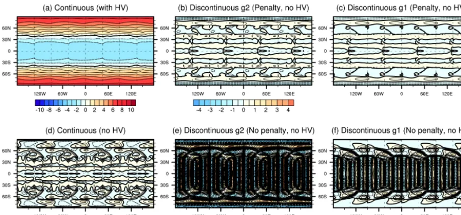
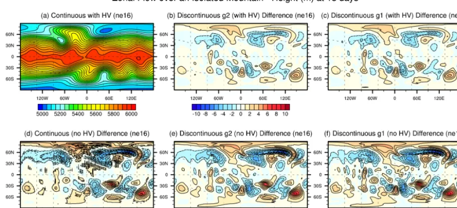
Figure 6. Height field with ne=16 andnp=4 at day 15 for zonal flow over an isolated mountain with (a) continuous elements and
hyperviscosity (reference solution). Height difference plot from reference solution withne=16 at day 15 for (b) discontinuousg2elements
with hyperviscosity, (c) discontinuousg1elements with hyperviscosity, (d) continuous elements without hyperviscosity, (e) discontinuous
g2elements without hyperviscosity and (f) discontinuousg1elements without hyperviscosity. The time step used for these runs was (a, d)
1t=480 s, (b, e)1t=240 s and (c, f)1t=120 s. Discontinuous penalization was used for both discontinuous schemes. Contour spacing is 1 m in all difference plots with the zero line removed. Long dashed lines show the cubed-sphere grid.
and (c) are quasi-mimetic, only losing energy conservation due to the discontinuous penalty term, and so exhibit very slow error growth with time. Simulations (e) and (f), which correspond to discontinuous elements without penalization, show greatly enhanced error norms and substantial imprint-ing from thene=4 pattern.
3026 P. A. Ullrich: A global finite-element shallow-water model
Discussion
P
ap
er
|
Dis
cussion
P
ap
er
|
Discussion
P
ap
er
|
Discussion
P
ap
er
|
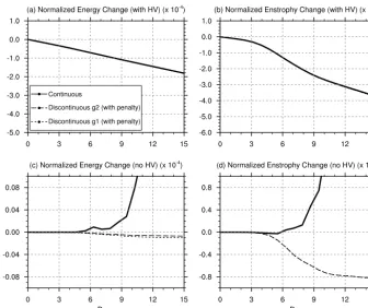
Fig. 7.
Normalized total energy and potential enstrophy change for the zonal flow over an isolated
moun-tain test with
n
e= 16
and
n
p= 4
over a 15 day simulation. In (a) all simulations show roughly equivalent
energy and enstrophy loss and so all lines are coincident. In (c) and (d) the simulation with continuous
elements is beginning to experience instability, leading to total energy and enstrophy growth after
ap-proximately 6 days simulation time.
42
Figure 7. Normalized total energy and potential enstrophy change for the zonal flow over an isolated mountain test withne=16 and
np=4 over a 15-day simulation. In (a) all simulations show roughly equivalent energy and enstrophy loss and so all lines are coincident. In
(c) and (d) the simulation with continuous elements is beginning to experience instability, leading to total energy and enstrophy growth after
approximately 6 days of simulation time.
Figure 8. Height field withne=16 andnp=4 at day 14 for the Rossby–Haurwitz wave with (a) continuous elements and hyperviscosity
(reference solution). Height difference plot from reference solution withne=16 at day 14 for (b) discontinuousg2elements with
hyper-viscosity, (c) discontinuousg1elements with hyperviscosity, (d) continuous elements without hyperviscosity, (e) discontinuousg2elements
without hyperviscosity and (f) discontinuousg1elements without hyperviscosity. The time step used for these runs was (a, d)1t=480 s,
(b, e)1t=200 s and (c, f)1t=120 s. Discontinuous penalization was used for both discontinuous schemes. Contour spacing is 1 m in plots
P. A. Ullrich: A global finite-element shallow-water model 3027
Discussion
P
ap
er
|
Dis
cussion
P
ap
er
|
Discussion
P
ap
er
|
Discussion
P
ap
er
|
Fig. 9.
Normalized total energy and potential enstrophy change for the Rossby-Haurwitz wave test with
n
e= 16
and
n
p= 4
over a 15 day simulation. In (a) and (b) all simulations show roughly equivalent
energy and enstrophy loss and so all lines are coincident. In (c) and (d) the simulation with
continu-ous elements is beginning to experience instability, leading to total energy and enstrophy growth after
approximately 6 days simulation time.
44
Figure 9. Normalized total energy and potential enstrophy change for the Rossby–Haurwitz wave test withne=16 andnp=4 over a 15-day
simulation. In (a) and (b) all simulations show roughly equivalent energy and enstrophy loss and so all lines are coincident. In (c) and (d) the simulation with continuous elements is beginning to experience instability, leading to total energy and enstrophy growth after approximately 6 days of simulation time.
but show stable error norms, discontinuous elements with penalization show smaller error norms than continuous ele-ments but a very slow growth with time due to the upwinding effect of the discontinuous penalization and discontinuous el-ements without penalization show rapid growth in errors (and even instability without mass lumping).
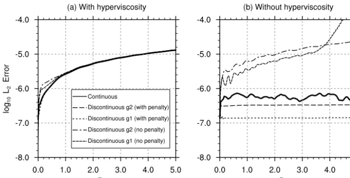
To verify that the model exhibits the correct convergence rate, Fig. 5 shows the global error norms associated with sim-ulations withne∈ {4,8,16,32,64}over a 5-day integration period. Atne=4, the time step is1t=2200 s for continu-ous elements,1t=800 s forg2discontinuous elements and
g1discontinuous elements with penalization, and1t=400 s forg1discontinuous elements without penalization. Increas-ing the time step by 100 s led to an unstable simulation. The time step is scaled inversely with increasing resolution. Missing simulations correspond to model instability and di-vergence prior to simulation completion. The use of hyper-viscosity reduces the convergence rate toO(1x3.2), as ex-pected from the choice of hyperviscosity coefficient, Eq. (44). With hyperviscosity disabled, model simulations con-verge at O(1x4) for continuous elements and discontinu-ous elements with penalty, and O(1x3)for discontinuous elements without penalty. The loss of 1 order of accuracy is due to one-sided differentiation at co-located nodes along element edges, leading to enhancement of the discontinuity.
Similar results (not shown) are observed when changingnp– that is, continuous elements and discontinuous elements with penalty converge atO(1xnp), whereas unpenalized
discon-tinuous elements converge atO(1xnp−1).
6.2 Zonal flow over an isolated mountain
Test case 5 in Williamson et al. (1992) considers zonal flow with underlying topography. The wind and height fields are defined as in section 6.1, except withh0=5960 m andu0= 20 m s−1, respectively. A conical mountain is used for the topographic forcing, given by
z=z0(1−r/R), (48)
with z0=2000 m, R=π/9 and r2=
min
R2, (λ−λc)2+(φ−φc)2. The center of the mountain is atλc=3π/2 andφc=π/6.
Simulation results for this test case were computed at
3028 P. A. Ullrich: A global finite-element shallow-water model
Discussion
P
ap
er
|
Dis
cussion
P
ap
er
|
Discussion
P
ap
er
|
Discussion
P
ap
er
|
Fig. 10.
Relative vorticity field with
n
e= 32
and
n
p= 4
at day 6 for the barotropic instability test with
(a) continuous elements and hyperviscosity (reference solution). Relative vorticity difference plot from
reference solution with
n
e= 16
at day 6 for (b) discontinuous
g
2elements with hyperviscosity, (c)
dis-continuous
g
1elements with hyperviscosity, (d) continuous elements without hyperviscosity, (e)
discon-tinuous
g
2elements without hyperviscosity and (f) discontinuous
g
1elements without hyperviscosity.
The time step used for these runs was (a,d)
∆
t
= 150
s, (b,e)
∆
t
= 75
s and (c,f)
∆
t
= 50
s.
Discontinu-ous penalization was used for both discontinuDiscontinu-ous schemes. Contour spacing in all plots is
2
×
10
−5s
−1with the zero line removed. Long dashed lines show the cubed-sphere grid.
45
Figure 10. Relative vorticity field withne=32 andnp=4 at day 6 for the barotropic instability test with (a) continuous elements and
hyperviscosity (reference solution). Relative vorticity difference plot from reference solution withne=16 at day 6 for (b) discontinuousg2
elements with hyperviscosity, (c) discontinuousg1elements with hyperviscosity, (d) continuous elements without hyperviscosity, (e)
dis-continuousg2elements without hyperviscosity and (f) discontinuousg1elements without hyperviscosity. The time step used for these runs
was (a, d)1t=150 s, (b, e)1t=75 s and (c, f)1t=50 s. Discontinuous penalization was used for both discontinuous schemes. Contour spacing in all plots is 2×10⁻⁵s−1with the zero line removed. Long dashed lines show the cubed-sphere grid.
so are instead compared against the continuous element run (with HV) in Fig. 6, where height fieldhand height field dif-ferenceh−hcare plotted (wherehcis the height field given in a). Simulations (b) and (c), corresponding to discontinuous elements with and without mass lumping, are very similar in structure and exhibit smooth differences from the continuous model. With no hyperviscosity applied, continuous elements (d) show significant noise which is not present for discontin-uous elements (e, f). These simulations match closely with results from the literature (Nair et al., 2005; Ullrich et al., 2010).
To understand conservation of invariants over time, total energy E and potential enstrophyξ are computed over the duration of the simulation. Since these quantities are invari-ant under the shallow-water equations, it would be expected that a perfect simulation would conserve these quantities ex-actly. They are defined via
E=1 2hv·v+
1 2gc(H
2−z2), and ξ=(ζ+f )2 2h . (49)
A time series of energy and potential enstrophy are plot-ted in Fig. 7. With hyperviscosity (a, b) all simulations ex-hibit nearly identical conservation properties, suggesting that both the continuous and discontinuous hyperviscosity opera-tors (which are responsible for the loss of energy and poten-tial enstrophy conservation) act in a nearly identical manner over the course of the simulation. Without hyperviscosity (c,
d) change in energy and potential enstrophy is much smaller. Continuous elements show initiation of instability at approx-imately day 6, likely due to high-wave-number oscillations in the height field caused by nonlinear aliasing. On the other hand, discontinuous elements instead show a slow decay of energy and potential enstrophy driven by the weak diffusivity of the discontinuous penalization.
6.3 Rossby–Haurwitz wave
Test case 6 in Williamson et al. (1992) consists of a westward-propagating Rossby–Haurwitz wave that exactly solves the barotropic vorticity equation, but only approxi-mately solves the nonlinear shallow-water equations. This test is particularly interesting since it is known to be sensi-tive to the choice of horizontal viscosity.
un-P. A. Ullrich: A global finite-element shallow-water model Discussion 3029
P
ap
er
|
Dis
cussion
P
ap
er
|
Discussion
P
ap
er
|
Discussion
P
ap
er
|
Fig. 11. Normalized total energy and enstrophy change for the barotropic instability test with ne=
16 andnp= 4over a 12 day simulation. In (c) and (d) the continuous element simulation fails after
approximately6days, leading to unbounded growth in energy and enstrophy. The time step used for these runs was (a,d)∆t= 300s, (b,e)∆t= 150s and (c,f)∆t= 75s. Discontinuous penalization was used for both discontinuous schemes.
46
Figure 11. Normalized total energy and enstrophy change for the barotropic instability test withne=16 andnp=4 over a 12-day simulation.
In (c) and (d) the continuous element simulation fails after approximately 6 days, leading to unbounded growth in energy and enstrophy. The time step used for these runs was (a, d)1t=300 s, (b, e)1t=150 s and (c, f)1t=75 s. Discontinuous penalization was used for both discontinuous schemes.
stable without the addition of hyperviscosity, whereas dis-continuous elements with penalization are effective at stabi-lizing the method for both lumped and non-lumped variants.
6.4 Barotropic instability
The barotropic instability test case of Galewsky et al. (2004) consists of a zonal jet with compact support at a latitude of 45◦, with a latitudinal profile roughly analogous to a much stronger version of test case 3 of Williamson et al. (1992). A small height perturbation is added atop the jet which leads to the controlled formation of an instability in the flow. The relative vorticity of the flow field at day 6 can then be vi-sually compared against a high-resolution numerically com-puted solution (Galewsky et al., 2004; St-Cyr et al., 2008).
Simulation results for this test case were computed at
ne=32 and np=4 after 12 days of integration with hy-perviscosity enabled. The time step used for these runs was
1t=150 s for continuous elements, 1t=75 s forg2 dis-continuous elements and1t=50 s forg1discontinuous el-ements. Increasing the time step by 10 s led to an unstable simulation. Simulations are again compared against the con-tinuous element run (with HV) in Fig. 10, where the relative vorticity fieldζ and relative vorticity field differenceζ−ζc
is plotted (where ζc is the height field given in a). Due to the presence of sharp frontal activity in this test case and the strong resolution dependence of this problem (Ullrich et al., 2010), differences inζ are of the same magnitude as the orig-inal field. In particular, the simulations without hyperviscos-ity (d, e, f) all show enhancement near wave fronts which is not apparent in the simulations with hyperviscosity (b, c). Al-though most differences can be found near sharp fronts, there is also a clear enhancement in the differences near 120 E as-sociated with a trailing instability. For continuous elements without hyperviscosity (c), there is also apparent grid-scale noise which is missing from the other simulations, suggest-ing that this method is under-diffused.
3030 P. A. Ullrich: A global finite-element shallow-water model 4), energy and potential enstrophy loss are significantly
re-duced compared to the simulations with hyperviscosity. Af-ter wave breaking, energy and potential enstrophy loss are of the same order of magnitude for simulations with and with-out hyperviscosity, associated with the fact that diffusivity is enhanced near the barotropic fronts where discontinuities are large.
7 Conclusions
Following Huynh (2007), a novel nodal finite-element method for continuous and discontinuous elements has been constructed using a robust derivative operator and discontin-uous penalization. The resulting methodology can be used for straightforward discretization of partial differential equa-tions in either a conservative or a non-conservative form. A hyperviscosity operator valid for both continuous and dis-continuous elements was also presented that would provide a mechanism for numerical stabilization and the removal of grid-scale noise. Two versions with discontinuous elements were studied, using either theg1org2flux correction func-tion for distribufunc-tion of boundary fluxes and penalty across nodal points. The resulting method was then applied to the 2-D shallow-water equations in cubed-sphere geometry and tested on a suite of test problems.
From the Williamson et al. (1992) test case suite, steady-state geostrophically balanced flow, zonal flow over an iso-lated mountain and the Rossby–Haurwitz wave were exam-ined, in addition to the barotropic instability test of Galewsky et al. (2004). The method was shown to be stable and accu-rate for both continuous and discontinuous elements, with fourth-order convergence being verified for cubic basis func-tions. Discontinuous penalization was shown to be necessary for stability and for maintaining the correct order of accu-racy of the discontinuous method. Overall the discontinuous elements required a smaller time step than for continuous el-ements, although all methods led to similar error norms when hyperviscosity was active. When hyperviscosity was deacti-vated, the discontinuous method exhibited better error norms than the continuous approach, and discontinuous penaliza-tion was shown to be sufficient for stability of the method even for complex flows. Nonetheless, differences between all three approaches appeared minor, and all methods performed well for this suite of tests.
The non-conservative discontinuous element formulation has been shown to be a potential candidate for future atmo-spheric modeling. It has the advantage of requiring fewer parallel communications than continuous methods, and hibits stability even when hyperviscosity is not used for ex-plicit stabilization. However, with the reduced time step size it remains unclear whether the discontinuous formulation would be computationally competitive with continuous el-ement methods.
P. A. Ullrich: A global finite-element shallow-water model 3031 Appendix A: Equivalence of differential and
variational forms
In this appendix equivalence of the variational formulation of the spectral element method and the differential formulation using the robust derivative is demonstrated. For continuous elements,f =f and Eq. (15) reduces to
Dαf (αi, βj)= np−1
X
p=0
f(p,j )
∂eφ(p)
∂α (αi), (A1)
which is simply the derivative of the continuous analogue to the nodal values alongβ=βj.
For simplicity consider a single quadrilateral spectral ele-ment with test functionsφij located at nodal points(αi, βj),
(i, j )∈ [0, . . ., np−1]2. The result is shown for an arbitrary 2-D conservation law,
∂ψ
∂t + ∇ ·F =0. (A2)
Using the derivative operator (A1), this equation reads as
∂ψij
∂t +
1
Jij
Dα(J Fα)+ 1
Jij
Dβ(J Fβ)=0, (A3) whereas under the variational formulation, (A2) is formu-lated as
Z ∂ψ
∂t φijdA+
Z
φij∇ ·FdA=0. (A4) Then using integration by parts,
X
m,n Z
φijφmndA ∂ψ
mn
∂t +B−
Z
∇φij·FdA=0, (A5)
whereBis the contribution due to the boundary which dis-appears under DSS. Introducing coordinates (α, β)with in-tegration on GLL nodes,
Z
fdA= np−1
X
s=0 np−1
X
t=0
fstJstwswt1α1β, (A6)
and so the first term of Eq. (A5) reads as X
m,n Z
φijφmndA ∂ψ
mn
∂t
=X
m,n
δi,mδj,nJijwiwj1α1β ∂ψmn
∂t
=Jijwiwj1α1β
∂ψij
∂t . (A7)
For the last term, observe that on a manifold ∇φij·F=gpqFp
gqr ∂φ ∂xr
=Fα∂φ ∂α+F
β∂φ
∂β, (A8)
and so Z
∇φij·FdA= np−1
X
s=0 np−1
X
t=0
Fα∂φij ∂α +F
β∂φij
∂β
α=αs,β=βt
Jstwswt1α1β. (A9)
On the other hand, by construction
∂φij
∂α = ∂eφ(i)
∂α eφ(j ), (A10)
andeφ(j )(βt)=δj t. This leads to Z
∇φij·FdA=
np−1
X
s=0
Fsjα∂eφ(i)
∂α (αs)Jsjwswj
+ np−1
X
t=0
Fitβ∂eφ(j )
∂β (βt)Jitwiwt
1α1β. (A11)
Furthermore, in conjunction with Eq. (A7), this can be written as
∂ψij
∂t −
1
Jij np−1
X
s=0
JsjFsjα
∂eφ(i)
∂α (αs) ws
wi
− 1
Jij np−1
X
t=0
JitFitβ
∂eφ(j )
∂β (βt) wt
wj
=0. (A12)
Equivalence of this equation with Eq. (A3) follows for a formulation on GLL nodes (Boyd, 2001, Appendix F), since these basis functions satisfy the property
∂eφ(i)
∂α (αs)ws= − ∂φe(s)
∂α (αi)wi. (A13)
Appendix B: Derivation of the viscosity operator In this appendix the derivation of the discrete viscosity op-erator is provided for scalar and vector hyperviscosity on a Riemannian manifold.
B1 Scalar viscosity
From the natural quadrature rule that arises from the nodal finite-element formulation, the left-hand side of Eq. (21) is discretized as
Z Z
f φ(i,j )dA= Z Z
feφ(i)(α)eφ(j )(β)dA
3032 P. A. Ullrich: A global finite-element shallow-water model and so, pointwise, theHoperator is applied via
f(i,j )=
ν
wiwj1α1βJ (αi, βj)
I
∂Z
φ(i,j )∇ψ·dS− Z Z
Z
∇φ(i,j )· ∇ψdA
. (B2)
The area integral term in Eq. (B2) is then computed: Z Z
∇φ(i,j )· ∇ψdA= Z Z
∇pφ∇pψdA= Z Z ∂φ
(i,j )
∂α ∇
αψ+∂φ(i,j )
∂β ∇
βψdA,
=1α1β
np−1 X
m=0 np−1
X
n=0 e
φ(j )
∂eφ(i)
∂α ∇
αψ J w mwn
α=α
m,β=βn
+1α1β
np−1 X
m=0 np−1
X
n=0 e
φ(i)
∂eφ(j )
∂β ∇
βψ J w mwn
α=αm,β=βn
(B3) =1α1βwj
np−1 X
m=0
∂eφ(i)
∂α ∇
αψ J w m
α=α
m,β=βj
+1α1βwi np−1
X
n=0
∂eφ(j )
∂β ∇
βψ J w n
α=α
i,β=βn.
From Eq. (B2), Eq. (23) then follows. The boundary inte-gral term in Eq. (21) takes the form
I
∂Z
φ(i,j )∇ψ·dS= Z
∂ZR
φ(i,j )∇ψ·dS
+ Z
∂ZT
φ(i,j )∇ψ·dS+ Z
∂ZL
φ(i,j )∇ψ·dS
+ Z
∂ZB
φ(i,j )∇ψ·dS, (B4)
whereR,T,LandBdenote the right, top, left and bottom edges, respectively. The quantity dS=Nd`denotes the nor-mal vector to the edge with magnitude equal to the infinites-imal length element. Only the covariant components of the face normals need to be known, at each edge given by
NpR=
1
√
gαα,0
, NpT = 0,p1 gββ
!
,
NpL=
−√1
gαα,0
, NpB= 0,− 1 p
gββ !
. (B5)
The infinitesimal length element along each edge is given by the covariant metric,
d`R=√gββdβ,d`T = √
gααdα,
d`L=√gββdβ,d`B= √
gααdα. (B6)
Then along the right edge, using the nodal discretization of the boundary integral,
Z
∂ZR
φ(i,j )∇ψ·dS=
δi,np−1
np−1 X
n=0 e
φ(j )(β)∇αψ NαRwn √
gββ1β
α=αnp−1,β=βn
=δi,np−1wj1β J∇
αψ
α=αnp−1,β=βj, (B7)
where we have usedgββ=J2gαα. Repeating for all edges and using Eq. (B2) then yields Eq. (24).
B2 Vector viscosity
The area integral that appears on the left-hand side of Eqs. (29) and (30) takes the form
Z Z
Z
f·φ(α)(i,j )dA= Z Z
Z
fαeφ(i)(α)eφ(j )(β)dA
=f(i,j )α wiwjJ 1α1β, (B8) Z Z
Z
f·φ(β)(i,j )dA= Z Z
Z
fβeφ(i)(α)eφ(j )(β)dA
=f(i,j )β wiwjJ 1α1β. (B9) B2.1 Discretization of the area integral
In nodal form, the divergence expands as
(∇ ·φ(α)(i,j ))= 1
J ∂ ∂α J g
ααφ (i,j )α
+1
J ∂ ∂β J g
βαφ (i,j )α
, (B10)
=eφ(j )(β)
J ∂ ∂α J g
αα e
φ(i)(α)
+eφ(i)(α)
J ∂ ∂β J g
βα e
φ(j )(β)
, (B11)
and so Z Z
Z
(∇ ·φ(i,j ))(∇ ·u)dA
=1α1β
np−1 X
m=0 np−1
X
n=0 "
e
φ(j )(βn)
J ∂ ∂α J g
αα e
φ(i)(α)
+eφ(i)(αm)
J ∂ ∂β J g
βα e
φ(j )(β)
(∇ ·u)J wmwn
=1α1βwj np−1
X
m=0
J gααdeφ(i)
dα (∇ ·u)wm
P. A. Ullrich: A global finite-element shallow-water model 3033
+1α1βwi np−1
X
n=0
J gβαdeφ(j )
dβ (∇ ·u)wn
α=α
i,β=βn
.
(B12) Further, the radial component of the vorticity expands as
(∇ ×φ(i,j ))r = −1
J ∂φ(i,j )α
∂β = −
e
φ(i)
J
deφ(j )
dβ , (B13)
and so Z Z
Z
(∇ ×φ(i,j ))r(∇ ×u)rdA
=1α1β np−1
X
m=0
np−1
X
n=0
"
−eφ(i)(αm) J
deφ(j )
dβ
#
(∇ ×u)rJ wmwn
α=α
m,β=βn
= −1α1βwi
np−1
X
n=0
deφ(j )
dβ (∇ ×u)rwn
α=α
i,β=βn
. (B14)
Combining Eqs. (B8), (B12) and (B14) then gives Eq. (32). An analogous procedure forβleads to Eq. (33). B2.2 Discretization of the boundary integral
Using Eqs. (B5)–(B6) and√gββ=J √
gαα, the contour in-tegral in Eq. (29) along the right edge becomes
Z
∂ZR
(∇ ·u)φ(α)(i,j )·dS=
δi,np−1(∇ ·u)g
ααJ w j1β
α=α
np−1,β=βj, (B15)
and along the top edge, also using√gαα=J p
gββ, Z
∂ZT
(∇ ·u)φ(α)(i,j )·dS=
δj,np−1(∇ ·u)g
αβJ w i1α
α=α
i,β=βnp−1. (B16)
Repeating for all edges and using Eq. (B8), the complete boundary integral for divergence damping then leads to the divergence damping contribution to Eq. (34). An analogous procedure for test functionφ(β)(i,j )leads to Eq. (35).
For vorticity damping, along the right edge, Eq. (30) reads as
Z
∂ZR
(∇ ×u)×φ·dS=
δi,np−1
βrα(∇ ×u)
rφ(i,j )αNβwj √
gββ1β
α=αnp−1,β=βj =0,
and along the top edge, Z
∂ZT
(∇ ×u)×φ·dS=
δj,np−1
βrα(∇ ×u)
rφ(i,j )αNβwi √
gαα1α
α=αi,β=βnp−1, =δj,np−1(∇ ×u)rwi1α.
3034 P. A. Ullrich: A global finite-element shallow-water model
Acknowledgements. The author would like to acknowledge Mark
Taylor, Oksana Guba, David Hall, Hans Johansen and Jorge Guerra for many fruitful conversations and for their assistance in refining this manuscript.
Edited by: H. Weller
References
Bao, L., Nair, R. D., and Tufo, H. M.: A mass and momen-tum flux-form high-order discontinuous Galerkin shallow wa-ter model on the cubed-sphere, J. Comput. Phys., 271, 224–243, doi:10.1016/j.jcp.2013.11.033, 2014.
Bates, J. R., Semazzi, F. H. M., Higgins, R. W., and Barros, S. R. M.: Integration of the shallow water equations on the sphere using a vector semi-Lagrangian scheme with a multigrid solver, Mon. Weather Rev., 118, 1615–1627, doi:10.1175/1520-0493(1990)118<1615:IOTSWE>2.0.CO;2, 1990.
Boyd, J.: The erfc-log filter and the asymptotics of the Euler and Vandeven sequence accelerations, in: Proceedings of the Third International Conference on Spectral and High Order Methods, edited by: Ilin, A. V. and Scott, L. R., 267–276, Houston, Journal of Mathematics, Houston, Texas, 1996.
Boyd, J. P.: Chebyshev and Fourier spectral methods, Courier Dover Publications, 2001.
Chen, C. and Xiao, F.: Shallow water model on cubed-sphere by multi-moment finite volume method, J. Comput. Phys., 227, 5019–5044, doi:10.1016/j.jcp.2008.01.033, 2008.
Chen, C., Li, X., Shen, X., and Xiao, F.: Global shallow water mod-els based on multi-moment constrained finite volume method and three quasi-uniform spherical grids, J. Comput. Phys., 271, 191– 223, doi:10.1016/j.jcp.2013.10.026, 2014.
Comblen, R., Legrand, S., Deleersnijder, E., and Legat, V.: A finite element method for solving the shallow wa-ter equations on the sphere, Ocean Model., 28, 12–23, doi:10.1016/j.ocemod.2008.05.004, 2009.
Côté, J. and Staniforth, A.: An accurate and efficient finite-element global model of the shallow-water equations, Mon. Weather Rev., 118, 2707–2717, doi:10.1175/1520-0493(1990)118<2707:AAAEFE>2.0.CO;2, 1990.
Dennis, J., Edwards, J., Evans, K. J., Guba, O. N., Lauritzen, P. H., Mirin, A. A., St-Cyr, A., Taylor, M. A., and Worley, P. H.: CAM-SE: A scalable spectral element dynamical core for the Commu-nity Atmosphere Model, Int. J. High Perform. Comput. Appl., 26, 74–89, doi:10.1177/1094342011428142, 2011.
Galewsky, J., Scott, R. K., and Polvani, L. M.: An initial-value problem for testing numerical models of the global shallow-water equations, Tellus Ser. A, 56, 429–440, doi:10.1111/j.1600-0870.2006.00192.x, 2004.
Giraldo, F., Hesthaven, J. S., and Warburton, T.: Nodal high-order discontinuous Galerkin methods for the spherical shallow water equations, J. Comput. Phys., 181, 499–525, 2002.
Gottlieb, S., Shu, C.-W., and Tadmor, E.: Strong stability-preserving high-order time discretization methods, SIAM review, 43, 89– 112, doi:10.1137/S003614450036757X, 2001.
Heikes, R. and Randall, D. A.: Numerical integration of the shallow water equations on a twisted icosahedral grid. Part I: Basic design and results of tests, Mon. Weather Rev., 123, 1862–1880,
doi:10.1175/1520-0493(1995)123<1862:NIOTSW>2.0.CO;2, 1995.
Hesthaven, J. S. and Warburton, T.: Nodal discontinuous Galerkin methods: Algorithms, analysis, and applications, vol. 54, Springer, 2007.
Huynh, H.: A flux reconstruction approach to high-order schemes including discontinuous Galerkin methods, AIAA paper, 4079, 42 pp., 2007.
Jakob-Chien, R., Hack, J. J., and Williamson, D. L.: Spectral trans-form solutions to the shallow water test set, J. Comput. Phys., 119, 164–187, doi:10.1006/jcph.1995.1125, 1995.
Läuter, M., Giraldo, F. X., Handorf, D., and Dethloff, K.: A dis-continuous Galerkin method for the shallow water equations in spherical triangular coordinates, J. Comput. Phys., 227, 10226– 10242, doi:10.1016/j.jcp.2008.08.019, 2008.
Li, X., Chen, D., Peng, X., Takahashi, K., and Xiao, F.: A multimoment finite-volume shallow-water model on the Yin Yang overset spherical grid, Mon. Weather Rev., 136, 3066, doi:10.1175/2007MWR2206.1, 2008.
Lin, S.-J. and Rood, R. B.: An explicit flux-form semi-Lagrangian shallow water model on the sphere, Q. J. Roy. Meteorol. Soc., 123, 2477–2498, doi:10.1002/qj.49712354416, 1997.
Nair, R. D., Thomas, S. J., and Loft, R. D.: A discontinuous Galerkin global shallow water model, Mon. Weather Rev., 133, 876–888, doi:10.1175/MWR2903.1, 2005.
Qaddouri, A., Pudykiewicz, J., Tanguay, M., Girard, C., and Côté, J.: Experiments with different discretizations for the shallow-water equations on a sphere, Q. J. Roy. Meteorol. Soc., 138, 989– 1003, doi:10.1002/qj.976, 2012.
Ringler, T., Ju, L., and Gunzburger, M.: A multiresolution method for climate system modeling: application of spherical cen-troidal Voronoi tessellations, Ocean Dynam., 58, 475–498, doi:10.1007/s10236-008-0157-2, 2008.
Ringler, T. D., Jacobsen, D., Gunzburger, M., Ju, L., Duda, M., and Skamarock, W. B.: Exploring a multiresolution modeling ap-proach within the shallow-water equations, Mon. Weather Rev., 139, 3348–3368, doi:10.1175/MWR-D-10-05049.1, 2011. Ritchie, H.: Application of the semi-Lagrangian method
to a spectral model of the shallow water equations,
Mon. Weather Rev., 116, 1587,
doi:10.1175/1520-0493(1988)116<1587:AOTSLM>2.0.CO;2, 1988.
Ronchi, C., Iacono, R., and Paolucci, P. S.: The “cubed sphere”: A new method for the solution of partial differential equa-tions in spherical geometry, J. Comput. Phys., 124, 93–114, doi:10.1006/jcph.1996.0047, 1996.
Rossmanith, J. A.: A wave propagation method for hyperbolic systems on the sphere, J. Comput. Phys., 213, 629–658, doi:10.1016/j.jcp.2005.08.027, 2006.
Ruuth, S.: Global optimization of explicit strong-stability-preserving Runge–Kutta methods, Math. Comput., 75, 183–207, 2006.
Sadourny, R.: Conservative finite-difference approximations of the primitive equations on quasi-uniform spherical grids,
Mon. Weather Rev., 100, 136–144,
doi:10.1175/1520-0493(1972)100<0136:CFAOTP>2.3.CO;2, 1972.
P. A. Ullrich: A global finite-element shallow-water model 3035
St-Cyr, A., Jablonowski, C., Dennis, J. M., Tufo, H. M., and Thomas, S. J.: A comparison of two shallow-water models with nonconforming adaptive grids, Mon. Weather Rev., 136, 1898– 1922, doi:10.1175/2007MWR2108.1, 2008.
Takahashi, Y. O., Hamilton, K., and Ohfuchi, W.: Explicit global simulation of the mesoscale spectrum of atmospheric motions, Geophys. Res. Lett., 33, L12812, doi:10.1029/2006GL026429, 2006.
Taylor, M., Tribbia, J., and Iskandarani, M.: The spectral element method for the shallow water equations on the sphere, J. Comput. Phys., 130, 92–108, doi:10.1006/jcph.1996.5554, 1997. Taylor, M. A. and Fournier, A.: A compatible and conservative
spec-tral element method on unstructured grids, J. Comput. Phys., 229, 5879–5895, doi:10.1016/j.jcp.2010.04.008, 2010.
Thomas, S. J. and Loft, R. D.: The NCAR spectral element cli-mate dynamical core: Semi-implicit Eulerian formulation, J. Sci. Comput., 25, 307–322, doi:10.1007/s10915-004-4646-2, 2005. Thuburn, J.: Some conservation issues for the dynamical cores of
NWP and climate models, J. Comput. Phys., 227, 3715–3730, doi:10.1016/j.jcp.2006.08.016, 2008.
Thuburn, J. and Woollings, T.: Vertical discretizations for compress-ible Euler equation atmospheric models giving optimal represen-tation of normal modes, J. Comput. Phys., 203, 386–404, 2005. Tolstykh, M. A.: Vorticity-divergence semi-Lagrangian
shallow-water model of the sphere based on compact finite differences, J. Comput. Phys., 179, 180–200, doi:10.1006/jcph.2002.7050, 2002.
Tolstykh, M. A. and Shashkin, V. V.: Vorticity–divergence mass-conserving semi-Lagrangian shallow-water model using the re-duced grid on the sphere, J. Comput. Phys., 231, 4205–4233, doi:10.1016/j.jcp.2012.02.016, 2012.
Ullrich, P. A.: Understanding the treatment of waves in atmospheric models. Part 1: The shortest resolved waves of the 1D linearized shallow-water equations, Q. J. Roy. Meteorol. Soc., 140, 1426– 1440, doi:10.1002/qj.2226, 2013.
Ullrich, P. A. and Jablonowski, C.: MCore: A non-hydrostatic atmospheric dynamical core utilizing high-order
finite-volume methods, J. Comput. Phys., 231, 5078–5108,
doi:10.1016/j.jcp.2012.04.024, 2012.
Ullrich, P. A., Jablonowski, C., and van Leer, B.: High-order finite-volume methods for the shallow-water equations on the sphere, J. Comput. Phys., 229, 6104–6134, doi:10.1016/j.jcp.2010.04.044, 2010.
Vincent, P. E., Castonguay, P., and Jameson, A.: A new class of high-order energy stable flux reconstruction schemes, J. Sci. Comput., 47, 50–72, doi:10.1007/s10915-010-9420-z, 2011. Williamson, D., Drake, J., Hack, J., Jakob, R., and Swarztrauber, P.:
A standard test set for numerical approximations to the shallow water equations in spherical geometry, J. Comput. Phys., 102, 211–224, doi:10.1016/S0021-9991(05)80016-6, 1992.